| Issue |
A&A
Volume 708, April 2026
|
|
|---|---|---|
| Article Number | A35 | |
| Number of page(s) | 9 | |
| Section | Planets, planetary systems, and small bodies | |
| DOI | https://doi.org/10.1051/0004-6361/202558036 | |
| Published online | 31 March 2026 | |
Investigating the Laplace plane transition theory for lunar chronology with a thermal-orbital coupled model
1
Southern University of Science and Technology,
518055,
Shenzhen, Guangdong,
China
2
University of California, Santa Cruz,
95064,
Santa Cruz, California,
USA
★ Corresponding author: This email address is being protected from spambots. You need JavaScript enabled to view it.
Received:
8
November
2025
Accepted:
30
January
2026
Abstract
The Moon may have formed from a giant impact with the initial Earth spinning fast about a highly tilted axis. In this case the subsequent orbital evolution causes the lunar orbit to go through instabilities during the Laplace plane transition (LPT). Based on this model it was suggested that the level of tidal heating in the Moon during the LPT is capable of explaining a predominance of lunar rock ages at ~4.35 Ga and the survival of older zircons; the heating in this period is enough to resurface much of the Moon, but not enough to reset the near-surface zircon chronology. However, this finding was based on estimates of heating rates using model orbital histories that did not consider the evolution of the Moon’s internal structure during tidal heating and the consequent feedback on orbital evolution. For this work we tested the previous theory using a coupled thermal-orbital model, and find that the peak heating rates are not significantly different from those previously determined (~1014–1015 W). In the case of a moderately dissipative Earth (Qe = 300), the typical duration of the heating event (up to 150–200 Myr) implies a Moon formation age of around 4.5 Ga, consistent with some lunar chronologies. We also provide an explanation for the quasiperiodic oscillation of lunar semimajor axis and eccentricity, which is characteristic of the LPT instability.
Key words: Moon / planets and satellites: dynamical evolution and stability / planets and satellites: formation
© The Authors 2026
 Open Access article, published by EDP Sciences, under the terms of the Creative Commons Attribution License (https://creativecommons.org/licenses/by/4.0), which permits unrestricted use, distribution, and reproduction in any medium, provided the original work is properly cited.
This article is published in open access under the Subscribe to Open model. This email address is being protected from spambots. You need JavaScript enabled to view it. to support open access publication.
1 Introduction
The Moon likely formed in the aftermath of a giant impact (Canup & Asphaug 2001; Canup et al. 2023). Simulations of the impact process (Ćuk & Stewart 2012; Canup 2012) suggest that the early Earth was spinning fast enough to allow the Moon to form primarily from terrestrial material, thus satisfying isotopic constraints (Wiechert et al. 2001; Zhang et al. 2012; Melosh 2014). The suggested spin rate implies a post-impact Earth–Moon system angular momentum that is about twice as large as the system’s present value. Mechanisms involving special situations of the Earth–Moon–Sun gravitational interactions have been proposed to remove this excess angular momentum, such as the evection resonance (Ćuk & Stewart 2012) and the evection-related limit cycle (Wisdom & Tian 2015; Tian et al. 2017; Rufu & Canup 2020).
Ćuk et al. (2016) instead proposed that the pre-impact proto-Earth’s spin axis had a big tilt, as much as 60°–70°. In this high-obliquity fast-spinning scenario, the excess angular momentum is drained during the instabilities associated with the Laplace plane transition (LPT). This transition occurs at the point where the influence of the Earth and the Sun on the precession of the Moon’s orbit are in balance. At sufficiently high obliquities (>68.9° in a simplified treatment; Tremaine et al. 2009), orbital instabilities arise. In the case that Earth started with a large tilt, the LPT produces large increases in the lunar orbit’s eccentricity and consequent high levels of tidal heating, a halt in the expansion of the Earth–Moon distance, and decreases in Earth’s spin rate, as angular momentum is transferred to the Earth–Moon barycenter’s solar orbit through gravitational interaction between the Sun and the Moon. As well as providing a separate pathway for draining the excess angular momentum, the high-obliquity scenario can also explain the present-day high inclination of the lunar orbit referenced to Earth’s equator. Tian & Wisdom (2020) found a constraint on the high-obliquity scenario that was not correctly modeled by (Ćuk et al. 2016): the perpendicular-to-ecliptic component of the Earth–Moon system’s initial angular momentum should equal the present value. Ćuk et al. (2016) reconsidered this constraint and updated the high-obliquity scenario, without finding any significant changes in the overall results.
Nimmo et al. (2024) further proposed, assuming that the Earth began in a high-obliquity fast-spinning state, that the tidal heating in the Moon during the LPT instability could have then provided enough power to reset most of the lunar chronometers (with the exception of near-surface zircons) and erased preexisting impact basins. In this scenario, the preponderance of lunar rock ages clustered around 4.35 Ga is due to tidal heating via the LPT at this time, and is not a reflection of when the Moon actually formed. However, this suggestion was based on calculations of tidal heating rates that assumed the lunar structure did not evolve with time (Ćuk et al. 2016, Tian & Wisdom 2020, Ćuk et al. 2021). Since an extreme tidal heating event would be expected to modify the internal lunar structure and potentially also the rate of tidal heating, it is important to consider whether such thermal-orbital feedback could invalidate the original hypothesis.
A Moon that is close to the Earth and in a very elliptical orbit experiences more severe tidal heating than a Moon that is farther away from the Earth and in a nearly circular orbit, resulting in differences of orders of magnitude in the lunar tidal heating rate. On the other hand, since the elastic and dissipative properties of the Moon are functions of its temperature and melt fraction, and these properties are key factors in determining the tidal accelerations of the Earth and Moon, the Moon’s thermal evolution affects the Earth-to-Moon relative velocity, and therefore orbital evolution through time.
An example of the importance of considering thermal-orbital feedback is as follows. It has been shown that the evection resonance, without considering feedback effects between the Moon’s orbital and thermal evolution, is capable of draining the excess angular momentum of the Earth–Moon system (Ćuk & Stewart 2012). However, a thermal-orbital coupled study (Tian et al. 2017) showed that the evection resonance is unstable due to over-heating of the Moon, and is thus insufficient to solve the angular momentum problem. Although a variety of works have considered the thermal-orbital coupled evolution of the Moon (e.g., Bierson & Nimmo 2016; Tian et al. 2017; Downey et al. 2023), none of them have studied the evolution through the LPT with a high-obliquity Earth.
In this study we investigated whether the hypothesis of tidal resetting of lunar chronology during the LPT is still viable when the coupling between orbital and thermal evolution is taken into account. It should be noted that this work is based on the assumption that the Earth–Moon system started with the Earth’s tilt being quite large, i.e., the high-obliquity scenario. Although some details of the behavior change under the influence of thermal-orbital feedback, we find that the peak heating rate and duration are not significantly different from earlier works (Ćuk et al. 2016, Tian & Wisdom 2020, Ćuk et al. 2021).
2 Model
The orbital model is based on the model described in Tian & Wisdom (2020). The major modification introduced here is to vary the elastic and dissipative properties of the Moon depending on its internal structure, where the elastic property is parameterized by the Moon’s degree-2 Love number k2m, and the dissipative property is parameterized by the dissipation quality factor Qm. Given the large uncertainties in the early state of the Moon, the model description of the lunar k2m-to-Qm ratio is kept deliberately simple, and is based on the assumption that the mechanical properties of the lunar interior are determined mainly by how much melt is present. Rheological experiments on silicates demonstrate that elastic moduli and dissipation are affected by the presence of melt (e.g., Jackson et al. 2004), with the effect on dissipation typically being more pronounced.
Our numerical model is based on the N-body symplectic mapping algorithm (Wisdom & Holman 1991); the mapping period is 1/40 of the lunar orbital period. The model includes (1) the three-body gravitational interactions between the Earth, the Moon, and the Sun; (2) the rotational mechanics of the Earth and the Moon, considering the spin-orbit interactions between each body with the orbit of the binary; (3) tidal deformations of both the Earth and the Moon, and the gravitational pulls caused by the tidal bulges; (4) the change in melt fraction in the lunar interior caused by the deposition of tidal heat in the mantle, as well as loss of heat through advection of melt to the surface; we ignore the heat loss through conduction to the surface as it is small compared to that from melt advection; (5) the changes in the Moon’s tidal parameters (k2m and Qm) caused by the evolving melt fraction of the mantle.
The mapping is an interleaving of a “drift” step that deals with integrable parts of the system (two-body motions, free rigid body rotations) and a “kick” step that deals with perturbations (spin-orbit interactions, Sun–Moon interaction, tides, and the melt evolution). The drift step reaches a precision of 10−12. For example, in solving Kepler’s equation which deals with converting the time increment to position increment, the error in the change in true anomaly is less than 10−12 rad over 1/40 of a lunar orbital time. The kick step only modifies the velocities and keeps the positions unchanged, and the issues of the choice of step size and how well the integration converges (in the kick step alone) do not exist; this is an intrinsic feature of the symplectic mapping method (Wisdom & Holman 1991). A mapping period of 1/20 of the shortest orbital period, i.e., the Moon’s period, is good enough, and we take it to be 1/40 to further constrain numerical errors. Orbital states are expressed in positions and Cartesian velocity components rather than orbital elements, and there is no special treatment for the Moon’s passage near pericenter.
The rigid body dynamics, including the free rotations and the spin-orbit interactions, are modeled using the Lie-Poisson algorithm, as described in Touma & Wisdom (1994). The mutual torques between Earth’s oblate figure and the Moon are the main cause of the lunar orbit’s pericenter precession and nodal precession before LPT. The mutual torques between the Moon’s triaxial figure and the Earth are important in that they have kept the Moon in synchronous rotation and in Cassini states over most, if not all, of the lunar history. However, the Moon’s spin-orbit torques have little influence on orbital motion since the moment of inertia of the orbit (taken to be mma2, where mm is the mass of the Moon and a is the lunar semimajor axis) is three to four orders of magnitude higher than that of the Moon (which is ![Mathematical equation: $\[{\sim}0.4 m_{m} R_{m}^{2}\]$](/articles/aa/full_html/2026/04/aa58036-25/aa58036-25-eq1.png) , where Rm = 1737 km is the radius of the Moon).
, where Rm = 1737 km is the radius of the Moon).
Regarding the shapes of the bodies, the Earth’s figure is updated in integrations by keeping J2e, the parameterization of Earth’s oblateness, proportional to the square of the Earth’s spin rate. On the other hand, we fix the Moon at its present-day figure, the same as the treatment in Tian & Wisdom (2020). Even though the lunar shape can strongly influence the Moon’s rotational dynamics, especially during the LPT instability (Ćuk et al. 2016) and the Cassini state transition (Matsuyama et al. 2021), the orbital evolution is not sensitive to the lunar shape parameters. This is manifested in the fact that Tian & Wisdom (2020) and Ćuk et al. (2016) obtained qualitatively similar orbital evolutionary behavior passing through the LPT, even though the latter considered a variable Moon shape, while the former did not. Therefore, though the adoption of a constant lunar figure in this study may not lead to definitive results regarding the Moon’s rotational behavior during the LPT, the credibility of the orbital evolution is reasonably unaffected. Furthermore, because the variations in the Moon’s rotation only affect the lateral distribution of tidal heating and do not alter the total heating rate, we expect the omission of a variable lunar shape would not change our conclusion regarding the magnitude of tidal heating. This is further discussed in Section 6.
The Mignard tidal model (Mignard 1981; Touma & Wisdom 1998) was used for the implementation of tides. This tidal model assumes a constant time lag between the position of the tidal bulge and the position of the tide-raising body that causes the bulge. For Earth’s tide, the time lag is Δte = 1/Qe/(ωe − n), where Qe is the Earth’s dissipative quality factor, ωe is the Earth’s spin rate, and n is the mean motion of the Moon. For tides on the Moon, the time lag is taken to be Δtm = 1/Qm/n. Compared to the Darwin–Kaula tidal model (Tian & Wisdom 2020), the latter considers dissipation in terms of phase lags in the arguments of trigonometries, which come along as the tidal potential energy is expanded to a Fourier series. The Mignard model does not require a Fourier expansion, nor a transformation between the position–velocity description of orbital state to the orbital elements description, resulting in a much simpler mathematical treatment. Nevertheless, it is as valid in representing tides, and would produce tidal evolution paths not significantly different from those given by the Darwin–Kaula model (Touma & Wisdom 1994).
The tidal parameters of the Moon are taken as functions of the melt fraction ϕ, where ϕ is taken to be the mean melt fraction of the silicate interior (Moore 2001; Bierson & Nimmo 2016):
![Mathematical equation: $\[k_{2 m}(\phi)=\frac{3 / 2}{1+\frac{19 \mu(\phi)}{2 \rho g R_m}},\]$](/articles/aa/full_html/2026/04/aa58036-25/aa58036-25-eq2.png) (1)
(1)
![Mathematical equation: $\[\mu(\phi)=\frac{\mu_0}{1+\frac{67}{15} \phi},\]$](/articles/aa/full_html/2026/04/aa58036-25/aa58036-25-eq3.png) (2)
(2)
![Mathematical equation: $\[k_{2 m}(\phi) / Q_m(\phi)=0.0007+0.04 \phi^2.\]$](/articles/aa/full_html/2026/04/aa58036-25/aa58036-25-eq4.png) (3)
(3)
Here Rm = 1737 km, ρ = 3338 kg/m3, and g=1.62 m/s2 are respectively the radius, density, and surface gravity of the Moon, and μ0 = 60 GPa is the reference rigidity.
Equation (1) is the standard expression for the tidal Love number of a uniform body (Munk & MacDonald 1960). This is a good approximation for the Moon, which has an iron core only 1% of the total mass of the Moon (Williams et al. 2014). Equation (2) calculates the dependence of shear modulus on the melt fraction, using the analytical approach described in Mavko (1980). These two equations are well justified in terms of the underlying physics. In contrast, the effect of melt on dissipation at tidal frequencies has proved hard to incorporate into a predictive model (Jackson et al. 2004). Rather than attempt to develop such a model, here we adopt a highly simplified description (Eq. (3)) based on two bodies of similar size for which observations are available: the Moon and Io. The essential aspects of Eq. (3) are that there is a background dissipation that applies to a completely solid body (ϕ = 0), and that the dissipation increases strongly as melt fraction increases.
Figure 1 shows how μ and the k2m-to-Qm ratio vary with ϕ based on Eqs. (2) and (3), respectively. The horizontal shaded regions are the measured k2m-to-Qm ratios of the present-day Moon (0.00064 ± 0.00007 according to Williams et al. 2014) and Io (0.015 ± 0.003 from Lainey et al. 2009). Equation (3) thus implies that the Moon is essentially melt-free at the present day. This conclusion is consistent with estimates based on thermal evolution modeling and conductivity profiles, although a deep partially molten layer may exist (Khan et al. 2014). For Io, Eq. (3) indicates a mean melt fraction in the range 0.5–0.7, which would in turn imply a k2m in the range 0.08–0.1. The melt fraction value is consistent with the lower bound of ϕ > 0.2 from induction experiments (Khurana et al. 2011) and the predicted k2m is consistent with that measured (k2m = 0.125 ± 0.047, Park et al. 2025). In using Io to constrain Eq. (3), we are implicitly assuming that the lunar mantle does not completely melt to form a magma ocean, but remains partially molten (as for Io; Park et al. 2025). Equation (3) is not a rigorously derived expression, but is meant to provide a simple demonstration of the extent to which tidal-orbital feedback affects tidal heating during passage through the LPT.
The rate of tidal heating (in units of W) for a satellite in synchronous rotation can be written (Wisdom 2008)
![Mathematical equation: $\[\begin{aligned}& P=\frac{21}{2} \frac{k_{2 m}}{Q_m} \frac{n^5 R_m^5}{G} \zeta\left(e, I_m\right)=\frac{21}{2} \frac{k_{2 m}}{Q_m} G^{3 / 2} m_e^{5 / 2} R_m^5 \frac{\zeta\left(e, I_m\right)}{a^{15 / 2}}, \\& \zeta\left(e, I_m\right)=\frac{2}{7} \frac{f_0(e)}{\beta^{15}}-\frac{4}{7} \frac{f_1(e)}{\beta^{12}} ~\cos~ I_m \\& \qquad\qquad+\frac{1}{7} \frac{f_2(e)}{\beta^9}\left(1+\left(\cos~ I_m\right)^2\right)+\frac{3}{14} \frac{e^2 f_3(e)}{\beta^{13}}\left(\sin~ I_m\right)^2 ~\cos (2 \Lambda), \\& f_0(e)=1+\frac{31}{2} e^2+\frac{255}{8} e^4+\frac{185}{16} e^6+\frac{25}{64} e^8, \\& f_1(e)=1+\frac{15}{2} e^2+\frac{45}{8} e^4+\frac{5}{16} e^6, \quad f_2(e)=1+3 e^2+\frac{3}{8} e^4, \\& f_3(e)=1-\frac{11}{6} e^2+\frac{2}{3} e^4+\frac{1}{6} e^6, \quad \beta=\left(1-e^2\right)^{1 / 2},\end{aligned}\]$](/articles/aa/full_html/2026/04/aa58036-25/aa58036-25-eq5.png) (4)
(4)
where G is the gravitational constant, me is the mass of the Earth, ![Mathematical equation: $\[n=\sqrt{G m_{e} / a^{3}}, e\]$](/articles/aa/full_html/2026/04/aa58036-25/aa58036-25-eq6.png) is the lunar orbital eccentricity, Im is the Moon’s obliquity to the lunar orbital plane, and Λ is the angle between the ascending node of the Moon’s equator on the orbital plane and the direction of pericenter. This expression is more complicated than the standard tidal heating expression (which is discussed below) because it takes into account the fact that lunar eccentricity and obliquity may both be high.
is the lunar orbital eccentricity, Im is the Moon’s obliquity to the lunar orbital plane, and Λ is the angle between the ascending node of the Moon’s equator on the orbital plane and the direction of pericenter. This expression is more complicated than the standard tidal heating expression (which is discussed below) because it takes into account the fact that lunar eccentricity and obliquity may both be high.
Wisdom (2008) also gave the expression of heating rate for asymptotic nonsynchronous rotation, which differs from Eq. (4) by replacing ζ(e, Im) with
![Mathematical equation: $\[\zeta_L\left(e, I_m\right)=\frac{2}{7}\left[\frac{f_0(e)}{\beta^{15}}-\frac{1}{\beta^{15}} \frac{f_1^2(e)}{f_2(e)} \frac{2 ~\cos ^2 I_m}{1+\cos ^2 I_m}\right].\]$](/articles/aa/full_html/2026/04/aa58036-25/aa58036-25-eq7.png) (5)
(5)
As we show in Sect. 6, the nonsynchronous rotation case typically produces slightly less heating than the synchronous case. Therefore, we adopted Eq. (4) for tidal heating even though the Moon may experience transient periods of nonsynchronous rotation.
The mean mantle melt fraction ϕ is subject to increase by tidal heating, which causes partial melting, and to decrease through melt ascension to the surface. Assuming that the melt is confined to a moderately shallow layer of thickness d = 400 km (Bierson & Nimmo 2016), then conservation of energy provides the following equation for the evolution of the mean melt fraction,
![Mathematical equation: $\[\frac{\mathrm{d} \phi}{\mathrm{~d} t} \approx \frac{H}{\rho L}-\frac{v_l}{d} \phi,\]$](/articles/aa/full_html/2026/04/aa58036-25/aa58036-25-eq8.png) (6)
(6)
where ![Mathematical equation: $\[H=P /\left(4 \pi R_{m}^{2} d\right)\]$](/articles/aa/full_html/2026/04/aa58036-25/aa58036-25-eq9.png) is the local heating rate (in units of W/m3), L = 3 × 10⁵ J kg−1 is the latent heat, and vl is the melt rise velocity. We follow Moore (2001) and assume that vl increases with melt fraction ϕ and also depends on the grain size, melt viscosity, and buoyancy, such that
is the local heating rate (in units of W/m3), L = 3 × 10⁵ J kg−1 is the latent heat, and vl is the melt rise velocity. We follow Moore (2001) and assume that vl increases with melt fraction ϕ and also depends on the grain size, melt viscosity, and buoyancy, such that
![Mathematical equation: $\[v_l=\gamma ~\phi^{N-1},\]$](/articles/aa/full_html/2026/04/aa58036-25/aa58036-25-eq10.png) (7)
(7)
where γ = 5 × 10⁻⁷ m/s is a characteristic velocity scale and N=3 is a constant relating the melt fraction to the permeability (see Moore 2001). We note that Eq. (6) makes the implicit assumption that the energy budget of the mantle is dominated by advection of melt, and not conduction or solid-state convection. For Io at the present day, this is certainly true (e.g., Moore 2001); for the early Moon the dominant mechanism is less obvious, but during the LPT we can show a posteriori that advection must have dominated (because the heat fluxes are so high).
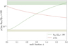 |
Fig. 1 Model for the variation in lunar rigidity μ and tidal dissipation factor k2m-to-Qm ratio as a function of melt fraction ϕ, using Eqs. (2) and (3). The olive and green horizontal shaded regions denote the measured k2m-to-Qm ratio values of the Moon (Williams et al. 2014) and Io (Lainey et al. 2009), respectively. |
3 Simulations and results
We assume the initial melt fraction to be ϕ = 0.2, implying a k2m-to-Qm ratio of about 0.0025 (Eq. (3)). We also carried out simulations with initial ϕ = 0.1 and 0.3, and found similar results as with initial ϕ = 0.2. The k2m-to-Qm ratio value is lower than the value of 0.01 typically adopted by Ćuk et al. (2016) and Tian & Wisdom (2020), but may be justified by the fact that the 0.01 value used previously was kept constant throughout each simulation, and therefore represents some kind of average. We wanted to investigate how an evolving k2m-to-Qm ratio affects the orbital evolution, and therefore began with a lower value to represent the Moon prior to an extreme tidal heating episode.
For the Earth, we assume its degree-2 Love number k2e = 0.3, and take two values for Qe: 300 and 30. The Q of the early Earth is very uncertain (e.g., Farhat et al. 2022; Korenaga & Marchi 2023), was certainly time-variable, and may have been controlled by the atmosphere’s ability to lose heat (Zahnle et al. 2015). The Qe value affects the rate at which the Moon recedes from the Earth. If the LPT theory for lunar chronology is correct, it requires that the Moon spends on the order of 100 Myr between the point of its formation at ~4.5 Ga (Schneider & Kleine 2025) and the point when it exits the LPT, when the LPT instability-related heating ceases. As we show below, such a timescale calls for a relatively nondissipative Earth, with Qe value nearer to the Qe = 300 endpoint. Nevertheless, the choice of Qe has little effect on the passage through the Laplace plane transition in general, and the peak tidal heating is only moderately higher in transient episodes in the endcase of Qe = 30.
For each choice of Qe, we start the system with three different initial conditions, i.e., with the Earth’s initial obliquity (Ie) being 61°, 65°, and 70°. The Earth’s initial spin rate is chosen such that the vertical angular momentum of the system matches that of the current Earth–Moon system. As in Tian & Wisdom (2020), these obliquity values represent the range of choices in the high-obliquity scenario, in that all three ultimately lead to instabilities during the LPT. All simulations are started with an Earth–Moon distance of 5 Re (the Earth’s Roche radius), where the Moon is assumed to have coalesced.
We first look at the case of Qe = 300, that is, a relatively nondissipative early Earth (Fig. 2). The three panels show simulations of the system started at Ie = 61°, 65°, and 70°. For each case, we also show a reference simulation that assumes a constant melt fraction of ϕ = 0.2 (i.e., k2m = 0.04538, Qm = 19.732 are constants, according to Eqs. (1)–(3)); we refer to these runs as the fixed-param case. Simulations that are subject to thermal-orbital feedback are shown as red curves, while the comparison fixed-param runs are shown in black. We note that tidal heating for the fixed-param cases is also calculated using the heating formula (Eq. (4)) for comparison.
In all these runs, the power of tidal heating during passage through the LPT peaks at the level of 1014–1015 W, the same as that obtained by both Ćuk et al. (2016) and Tian & Wisdom (2020), and indicates that the fundamental behavior of the LPT is unchanged by incorporating thermal-orbital coupling. From our perspective, this is a key result. Even though our coupling model is simplified, it indicates that a period of extreme tidal heating is a robust consequence of passage through the LPT, suggesting that the resetting of most lunar chronometers by such a passage – as Nimmo et al. (2024) suggests – is allowable.
Another important result is that the Moon stays trapped in a high heating state for substantial periods of time: in the top two panels, the heating rate does not drop below 1014 W until ~150 and 200 Myr after the simulation starts. Since the lunar age cluster at 4.35 Ga is presumed to represent the end of the tidal heating periods, these results imply a formation age for the Moon of 4.5–4.55 Ga, consistent with some geochronometers (e.g., Schneider & Kleine 2025).
Some of the runs terminate early because the lunar orbit becomes hyperbolic. In the nonhyperbolic cases we see that the lunar eccentricity frequently experiences quick increases to large values (e.g., 0.5). When the eccentricity exceeds 1, the Moon escapes. The occurrence of the hyperbolic ejection of the Moon during the Laplace plane transition instability is a matter of probability. Given the same initial obliquity, the Moon may or may not escape depending on different initial orientations of the Moon adopted (as expressed in terms of the Moon’s initial longitude of ascending node, argument of pericenter, and mean anomaly). The fact that our Moon is still here at present means that our Moon did not take the evolutionary path represented by hyperbolic scenarios.
Although the LPT theory for lunar chronology favors a relatively nondissipative early Earth, we also carried out simulations with a dissipative Earth of Qe = 30 (Fig. 3) to see how this change can affect heating. The results are qualitatively similar, with moderately high values for peak heating rates. In detail, the changes are the following: (1) The peak heating rate librates mainly between 1014 and 1016 W, compared to the Qe = 300 case where the peak is closer to 1014 W. (2) There are more frequent transient periods when the peak heating rate briefly exceeds 1016 W; however, they typically last for ~10 kyr and are separated by 0.5–1 Myr. (3) The evolution through the LPT takes a shorter time, because Qe, the dissipative quality factor of the Earth, is the dominant factor in determining the rate of orbital expansion. Heating typically ceases after a few tens of megayears, which in the LPT hypothesis would imply a Moon formation timescale in the range 4.4–4.35 Gyr, less consistent with most lunar chronologies. (4) As a consequence of the Earth being more dissipative, the quasiperiodic oscillations in a and e (as described in the next section) have much shorter periods.
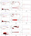 |
Fig. 2 Simulations with Qe = 300, showing three cases with different initial Earth obliquities (61°, 65°, and 70°). In each panel, the lower middle subfigure shows h vs. time, where h is the difference between the longitudes of ascending nodes of Earth’s equator and the lunar orbit, both measured on the ecliptic plane. The angle h is a natural measure of whether the lunar orbit is aligned to Earth’s equator. During the LPT, the amplitude of h gradually grows from near-zero to π. |
4 Quasiperiodic oscillations
In the cases shown we see the frequent occurrence of a quasiperiodic behavior: the lunar eccentricity, semimajor axis, and tidal heating rate often exhibit oscillations in a quasiperiodic manner during the LPT instability. In particular, this oscillation is manifested in the sawtooth shape of the semimajor axis versus time curve shown in Fig. 3c (Qe = 30, initial obliquity being 70°); we show this oscillation in more detail in Fig. 4 (the fixed-param case, first 10 Myr).
The fact that this oscillation occurs in the constant k2m-to-Qm ratio case shows that it is not a consequence of thermal-orbital feedback, which can also induce oscillations (Ojakangas & Stevenson 1986). Rather, this oscillation is due to a negative feedback between the lunar orbit’s semimajor axis (a) and eccentricity (e), both as functions of time: a = a(t), e = e(t).
On the one hand, the rate of change of the semimajor axis is dependent on the value of eccentricity through tides. The Article number, page 6 of 9 tidal rates of a(t) and e(t), according to Wisdom & Tian (2015), Eqs. (21)–(28) (where the obliquity tides are neglected), are
![Mathematical equation: $\[\dot{a}=\frac{2}{3} K a\left[1-\left(7 A-\frac{51}{4}\right) e^2-\left(\frac{403}{8} A-\frac{1065}{16}\right) e^4+\cdots\right],\]$](/articles/aa/full_html/2026/04/aa58036-25/aa58036-25-eq11.png) (8)
(8)
![Mathematical equation: $\[\dot{e}=-\frac{1}{3} K\left[\left(7 A-\frac{19}{4}\right) e+\left(\frac{347}{8} A-\frac{503}{16}\right) e^3+\cdots\right],\]$](/articles/aa/full_html/2026/04/aa58036-25/aa58036-25-eq12.png) (9)
(9)
where
![Mathematical equation: $\[K \propto a^{-13 / 2}, \quad A=\frac{k_{2 m} / Q_m}{k_{2 e} / Q_e}\left(\frac{m_e}{m_m}\right)^2\left(\frac{R_m}{R_e}\right)^5,\]$](/articles/aa/full_html/2026/04/aa58036-25/aa58036-25-eq13.png) (10)
(10)
and Re is the radius of the Earth.
In the fixed-param run, the tidal parameters are constants: k2m = 0.04538, Qm = 19.73213, k2e = 0.3, Qe = 30; the A parameter is also constant: A = 2.29. Then the equation regarding ![Mathematical equation: $\[\dot{a}\]$](/articles/aa/full_html/2026/04/aa58036-25/aa58036-25-eq14.png) becomes
becomes
![Mathematical equation: $\[\dot{a} \propto 1-3.27 e^2-48.75 e^4+\cdots,\]$](/articles/aa/full_html/2026/04/aa58036-25/aa58036-25-eq15.png) (11)
(11)
So there is a critical eccentricity: ecrit = 0.337. When e < ecrit, a increases; when e > ecrit, a decreases. This analysis explains where the turning points of the sawtooth shape are located. Whenever e(t) grows above ecrit, a(t) starts to decrease, thus resulting in a peak of a(t), as shown by the yellow triangles in Fig. 4.
On the other hand, the occurrence of increases in eccentricity is regulated by the value of the semimajor axis through LPT-related instabilities. With Eq. (9) alone and the parameter value A = 2.29, we see that ![Mathematical equation: $\[\dot{e}\]$](/articles/aa/full_html/2026/04/aa58036-25/aa58036-25-eq16.png) should always be negative. However, when the system approaches the LPT location with Earth having a big tilt, LPT-related instabilities drive the eccentricity to increase.
should always be negative. However, when the system approaches the LPT location with Earth having a big tilt, LPT-related instabilities drive the eccentricity to increase.
As noted above, the LPT is a time when perturbations on the Moon’s orbital evolution from the Earth’s oblate shape and the Sun are approximately equal in strength. When the Moon is very close to Earth, i.e., when a is small, the Earth oblateness perturbation dominates, and when a is large (like the present), the Sun’s influence dominates. So there exists a critical distance, acrit, at which the systems enters the Laplace plane transition.
According to Tremaine (2023) Eq. (5.74) and Nicholson et al. (2008) Eq. (3), the critical semimajor axis, when Earth’s orbit around the Sun is assumed to be circular, is
![Mathematical equation: $\[a_{\mathrm{crit}}=\xi(I_e, h_{\max}) \cdot r_L, \qquad r_L^5=\frac{J_{2 e} m_e R_e^2}{m_s} a_e^3,\]$](/articles/aa/full_html/2026/04/aa58036-25/aa58036-25-eq17.png) (12)
(12)
where ms is the mass of the Sun, ae is the Earth–Sun distance, hmax is the amplitude of libration of h (see caption of Fig. 2). The factor ξ(Ie, hmax) can be understood with Fig. 5. For the green curve in Fig. 4, ξ = 0.87, and this choice of value is explained as follows.
Figure 5 shows the shape of the Laplace surface, as measured by its deviation from the Earth’s equator (ε), as a function of Earth’s equatorial tilt (Ie) and the lunar semimajor axis (a). The Laplace plane is the plane such that if the Moon’s orbit were to lie on it, then the orbital plane would not precess since the would-be axis of precession coincides with the orbit normal. When a ≪ rL, the Laplace surface coincides with Earth’s equator (so ε ≈ 0). When a ≫ rL, the Laplace surface coincides with the ecliptic (so ε ≈ Ie). So rL is a useful lengthscale for determining whether the system has passed the LPT. However, it is useful only in an order of magnitude sense, instead of the accurate sense. The Laplace surface clearly deviated from the Earth’s equator before a reached rL (i.e., before a/rL reached 1). In other words, the LPT is a continuous process over a distance range, instead of a sudden transition at a = rL. Therefore, the triggering of the LPT instability need not occur at a = rL, but likely before that point (i.e., ξ < 1). With the exact distance represented by ξrL, the ξ factor depends on Ie, and on how much the lunar orbital plane deviates from the Earth’s equator plane, which is indicated by hmax, the amplitude of the libration of the angle h. For the case of Figs. 3c and 4, the ξ factor is heuristically taken to be 0.87.
Since the Earth is more oblate at higher spin rates, and since Earth’s spin rate constantly declines, J2e is monotonically decreasing. Consequently, the decline in acrit value as seen in Fig. 4 is an expected outcome of Eq. (12).
The existence of a critical semimajor axis for the onset of the LPT instability explains why eccentricity always plunges to near zero shortly after a(t) begins to decrease: a(t) drops below acrit, and the system leaves the LPT. As a result, the LPT-related instabilities (which cause the eccentricity to increase) cease, and the evolution of e(t) is then controlled by tides alone. Since ![Mathematical equation: $\[\dot{e}\]$](/articles/aa/full_html/2026/04/aa58036-25/aa58036-25-eq18.png) from tides is always negative (Eq. (9)), e(t) drops to and stays near zero, as shown by the green triangles in Fig. 4. This also explains why the eccentricity always rises again not long after it plunges to zero: since a is steadily increasing due to e being near-zero (Eq. (8)), when a(t) exceeds acrit, the system enters the LPT again, and the LPT-related instabilities start exciting the eccentricity. This is shown by the red triangles in Fig. 4.
from tides is always negative (Eq. (9)), e(t) drops to and stays near zero, as shown by the green triangles in Fig. 4. This also explains why the eccentricity always rises again not long after it plunges to zero: since a is steadily increasing due to e being near-zero (Eq. (8)), when a(t) exceeds acrit, the system enters the LPT again, and the LPT-related instabilities start exciting the eccentricity. This is shown by the red triangles in Fig. 4.
These two mechanisms together form a negative feedback between a(t) and e(t), which serves as the driver of the sawtooth shape of the semimajor axis versus time curve. We use the process shown in the right panel of Fig. 4 as an example: (1) from a state with e ≈ 0 and a < acrit, tides cause a(t) to grow; when a > acrit, e begins to substantially increase, as marked by the red triangles; (2) e continues to increase until it reaches ecrit, at which point a also reaches its peak value; after this point, a begins to decrease, while e may continue to get bigger and reach an equilibrium value determined by the competition between tides and the LPT instability, as marked by the yellow triangles; (3) a decreases until it falls below acrit, at which point e begins to decrease substantially, and the system soon comes to state (1), as marked by the green triangles.
The feedback loop repeats itself until the amplitude of the angle h reaches π, beyond which point the lunar orbital plane is no longer aligned to Earth’s equator in any sense, but instead precesses about the ecliptic. This is when system has completed the Laplace plane transition.
In terms of the rate of tidal heating in the Moon, this oscillation both causes a quasiperiodic pattern in the temporal change of heating, and stabilizes the peak heating rates. The heating rate is quasiperiodic because the rate is a function of e and a (Eq. (4)); more specifically, it correlates positively with e and negatively with a. The peak heating rates are stabilized because heating can be high only when the conditions of a large e and a small a are both satisfied, and this combination is never possible in the quasiperiodic oscillations of a and e. In Fig. 4, for example, the phase after the green triangle and before the red triangle is characterized by small e and small a; for this analysis we ignore the contribution of Im in Eq. (4) since at most times Im is close to zero. The phase after the red triangle and before the green triangle is characterized by large e and large a, so the combination of large e and small a would never appear. As a consequence, the peak tidal heating rate remains in the range 1014–1015 W, and does not depend on whether or not thermal-orbital feedback is taken into account.
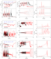 |
Fig. 3 As for Fig. 2, but with Qe = 30. Initial Earth obliquities are (a) 61 degrees, upper subplot; (b) 65 degrees, middle subplot; (c) 70 degrees, lower subplot. |
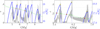 |
Fig. 4 Detailed view of the quasiperiodic oscillations for the simulation with Qe = 30. The initial obliquity is 70° (Fig. 3c, the fixed-param case). The gray dashed line shows the critical eccentricity ecrit = 0.337. The green curve shows the critical semimajor axis acrit over time. |
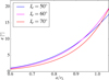 |
Fig. 5 Shape of the Laplace surface for three different values of the Earth’s obliquity Ie, adapted from Tremaine (2023) Fig. 5.3. The vertical axis ε is the angle between the Laplace surface and the Earth’s equator plane. |
5 Brief interlude of evection resonance
In some cases, such as the case shown in Fig. 3c, the system goes through a brief early interlude of passing through the evection resonance, causing a short-lived, but strong increase in eccentricity, heating, and melt production. The first 100 kyr of Fig. 3c is shown in detail in Fig. 6.
This interlude produces tidal heating rates much higher than in the much later LPT stage, reaching 1017 to 1018 watts. In reality, such high heating rates are probably enough to completely melt the entire Moon and are not well described by our simple model (Eq. (3)). However, since capture into the evection resonance happened at the very beginning of lunar history (when a ≈ 7Re), and in addition, only for a brief duration (10 kyr to 50 kyr), this brief interlude would essentially be indistinguishable from the processes taking place immediately after the formation of the Moon and would have had no effect on chronological markers recording events tens or hundreds of megayears later.
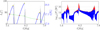 |
Fig. 7 Left: lunar obliquity Im for the same simulation case as shown in Figs. 3c and 4. Right: difference in tidal heating rates given by Eqs. ((4), gray), ((5), red), and ((13), blue). |
6 Obliquity tidal heating
Previous studies (e.g., Tian et al. 2017; Nimmo et al. 2024) did not consider the contribution of obliquity tides to lunar tidal heating. Consequently, the dependence of tidal heating P on lunar obliquity Im was ignored, and the approximate formula (Murray & Dermott 1999) was used:
![Mathematical equation: $\[P \approx \frac{21}{2} \frac{k_{2 m}}{Q_m} \frac{n^5 R_m^5}{G} e^2=\frac{21}{2} \frac{k_{2 m}}{Q_m} G^{3 / 2} m_e^{5 / 2} R_m^5 \frac{e^2}{a^{15 / 2}}.\]$](/articles/aa/full_html/2026/04/aa58036-25/aa58036-25-eq19.png) (13)
(13)
However, during the LPT instability, which is a three-dimensional process, the lunar obliquity frequently becomes high, sometimes as high as nearly 180° (i.e., temporary near-retrograde rotation relative to the lunar orbit), as shown in Fig. 7. Even though Im stays near zero for most of the time, it is usually excited for a ~10 kyr transient period shortly after the semimajor axis reaches a peak and starts to decline. The omission of obliquity tidal heating can result in an underestimate of the overall heating rate by about one order of magnitude during such transient periods.
Figure 7 also shows the heating rate as given by Eq. (5), where the Moon’s rotation becomes nonsynchronous when Im becomes very high. We see that the consideration of the nonsynchronous equation does not push the heating rate any further.
We note that due to our adoption of the Moon’s present-day figure, and the sensitivity of the Moon’s rotational dynamics to its figure, the presence of transient periods of high lunar obliquity in our results should not be regarded as an accurate depiction of this phenomenon. This discussion is more of an attempt to assess whether, and to what extent, obliquity tidal heating can affect our conclusions regarding the overall heating during possible extreme situations.
7 Conclusion
In this paper we investigated how the orbital evolution of the Moon during the Laplace Plane transition is influenced by thermal-orbital feedback. At least for the simplified model we adopted, the resulting peak heating rates are very similar to those found by earlier studies assuming constant lunar properties. In the case of a moderately dissipative Earth (Qe = 300), the typical duration of the heating event (up to 150–200 Myr) implies a Moon formation age of around 4.5 Ga, consistent with some lunar chronologies. We conclude that the Laplace plane transition instability provides a viable potential explanation for the chronology of lunar rocks, even considering the feedback between the orbital evolution and the thermal and magmatic activity of the lunar interior.
Acknowledgements
We thank Matija Ćuk for insightful remarks.
References
- Bierson, C. J., & Nimmo, F. 2016, J. Geophys. Res. Planets, 121, 2211 [Google Scholar]
- Canup, R. M. 2012, Science, 338, 1052 [NASA ADS] [CrossRef] [Google Scholar]
- Canup, R. M., & Asphaug, E. 2001, Nature, 412, 708 [Google Scholar]
- Canup, R. M., Righter, K., Dauphas, N., et al. 2023, Rev. Mineral. Geochem., 89, 53 [Google Scholar]
- Ćuk, M., & Stewart, S. T. 2012, Science, 338, 1047 [CrossRef] [Google Scholar]
- Ćuk, M., Hamilton, D. P., Lock, S. J., & Stewart, S. T. 2016, Nature, 539, 402 [CrossRef] [Google Scholar]
- Ćuk, M., Lock, S. J., Stewart, S. T., & Hamilton, D. P. 2021, Planet. Sci. J., 2, 147 [Google Scholar]
- Downey, B. G., Nimmo, F., & Matsuyama, I. 2023, Icarus, 389, 115257 [Google Scholar]
- Farhat, M., Auclair-Desrotour, P., Boué, G., & Laskar, J. 2022, A&A, 665, L1 [NASA ADS] [CrossRef] [EDP Sciences] [Google Scholar]
- Jackson, I., Faul, U. H., Fitz Gerald, J. D., & Tan, B. H. 2004, J. Geophys. Res., 109, B06201 [Google Scholar]
- Khan, A., Connolly, J. A. D., Pommier, A., & Noir, J. 2014, J. Geophys. Res. Planets, 119, 2197 [Google Scholar]
- Khurana, K. K., Jia, X., Kivelson, M. G., et al. 2011, Science, 332, 1186 [Google Scholar]
- Korenaga, J., & Marchi, S. 2023, Proc. Natl. Acad. Sci., 120, e2309181120 [Google Scholar]
- Lainey, V., Arlot, J.-E., Karatekin, Ö., & van Hoolst, T. 2009, Nature, 459, 957 [Google Scholar]
- Matsuyama, I., Trinh, A., & Keane, J. T. 2021, Planet. Sci. J., 2, 232 [Google Scholar]
- Mavko, G. M. 1980, J. Geophys. Res. Solid Earth, 85, 5173 [Google Scholar]
- Melosh, H. J. 2014, Phil. Trans. R. Soc. A, 372, 1 [Google Scholar]
- Mignard, F. 1981, Moon Planets, 24, 189 [Google Scholar]
- Moore, W. B. 2001, Icarus, 154, 548 [Google Scholar]
- Munk, W. H., & MacDonald, G. J. F. 1960, The Rotation of the Earth (London: Cambridge University Press) [Google Scholar]
- Murray, C. D., & Dermott, S. F. 1999, Solar System Dynamics (New York, NY: Cambridge University Press) [Google Scholar]
- Nicholson, P. D., Ćuk, M., Sheppard, S. S., Nesvorný, D., & Johnson, T. V. 2008, in The Solar System Beyond Neptune (Tucson, AZ: University of Arizona Press), 411 [Google Scholar]
- Nimmo, F., Kleine, T., & Morbidelli, A. 2024, Nature, 636, 598 [Google Scholar]
- Ojakangas, G. W., & Stevenson, D. J. 1986, Icarus, 66, 341 [Google Scholar]
- Park, R. S., Jacobson, R. A., Gomez Casajus, L., et al. 2025, Nature, 638, 69 [Google Scholar]
- Rufu, R., & Canup, Robin M. 2020, J. Geophys. Res. Planets, 125, e2019JE006312 [Google Scholar]
- Schneider, Jonas M., & Kleine, T. 2025, Earth Planet. Sci. Lett., 669, 119592 [Google Scholar]
- Tian, Z. L., & Wisdom, J. 2020, Proc. Natl. Acad. Sci., 117, 15460 [Google Scholar]
- Tian, Z. L., Wisdom, J., & Elkins-Tanton, L. 2017, Icarus, 281, 90 [Google Scholar]
- Touma, J., & Wisdom, J. 1994, AJ, 108, 1943 [NASA ADS] [CrossRef] [Google Scholar]
- Touma, J., & Wisdom, J. 1994, AJ, 107, 1189 [Google Scholar]
- Touma, J., & Wisdom, J. 1998, AJ, 115, 1653 [NASA ADS] [CrossRef] [Google Scholar]
- Tremaine, S. 2023, Dynamics of Planetary Systems (Princeton, NJ: Princeton University Press) [Google Scholar]
- Tremaine, S., Touma, J., & Namouni, F. 2009, AJ, 137, 3706 [Google Scholar]
- Wiechert, U., Halliday, A. N., Lee, D. C., et al. 2001, Science, 294, 345 [CrossRef] [Google Scholar]
- Williams, J. G., Konopliv, A. S., Boggs, D. H., et al. 2014, J. Geophys. Res. Planets, 119, 1546 [NASA ADS] [CrossRef] [Google Scholar]
- Wisdom, J. 2008, Icarus, 193, 637 [Google Scholar]
- Wisdom, J., & Holman, M. 1991, AJ, 102, 1528 [Google Scholar]
- Wisdom, J., & Tian, Z. 2015, Icarus, 256, 138 [Google Scholar]
- Zahnle, K., Lupu, R., Dobrovolskis, A., & Sleep, N. 2015, Earth Planet. Sci. Lett., 427, 74 [CrossRef] [Google Scholar]
- Zhang, J., Dauphas, N., Davis, A., Leya, I., & Fedkin, A. 2012, Nat. Geosci., 5, 251 [NASA ADS] [CrossRef] [Google Scholar]
All Figures
|
Fig. 1 Model for the variation in lunar rigidity μ and tidal dissipation factor k2m-to-Qm ratio as a function of melt fraction ϕ, using Eqs. (2) and (3). The olive and green horizontal shaded regions denote the measured k2m-to-Qm ratio values of the Moon (Williams et al. 2014) and Io (Lainey et al. 2009), respectively. |
| In the text | |
|
Fig. 2 Simulations with Qe = 300, showing three cases with different initial Earth obliquities (61°, 65°, and 70°). In each panel, the lower middle subfigure shows h vs. time, where h is the difference between the longitudes of ascending nodes of Earth’s equator and the lunar orbit, both measured on the ecliptic plane. The angle h is a natural measure of whether the lunar orbit is aligned to Earth’s equator. During the LPT, the amplitude of h gradually grows from near-zero to π. |
| In the text | |
|
Fig. 3 As for Fig. 2, but with Qe = 30. Initial Earth obliquities are (a) 61 degrees, upper subplot; (b) 65 degrees, middle subplot; (c) 70 degrees, lower subplot. |
| In the text | |
|
Fig. 4 Detailed view of the quasiperiodic oscillations for the simulation with Qe = 30. The initial obliquity is 70° (Fig. 3c, the fixed-param case). The gray dashed line shows the critical eccentricity ecrit = 0.337. The green curve shows the critical semimajor axis acrit over time. |
| In the text | |
|
Fig. 5 Shape of the Laplace surface for three different values of the Earth’s obliquity Ie, adapted from Tremaine (2023) Fig. 5.3. The vertical axis ε is the angle between the Laplace surface and the Earth’s equator plane. |
| In the text | |
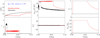 |
Fig. 6 First 100 kyr of the simulation in Fig. 1c. Evection resonances are encountered. |
| In the text | |
Current usage metrics show cumulative count of Article Views (full-text article views including HTML views, PDF and ePub downloads, according to the available data) and Abstracts Views on Vision4Press platform.
Data correspond to usage on the plateform after 2015. The current usage metrics is available 48-96 hours after online publication and is updated daily on week days.
Initial download of the metrics may take a while.