| Issue |
A&A
Volume 708, April 2026
|
|
|---|---|---|
| Article Number | A46 | |
| Number of page(s) | 18 | |
| Section | Extragalactic astronomy | |
| DOI | https://doi.org/10.1051/0004-6361/202558552 | |
| Published online | 26 March 2026 | |
NOCTURNE
I. The radio spectrum of narrow-line Seyfert 1 galaxies
1
European Southern Observatory (ESO), Alonso de Córdova 3107, Casilla 19 Santiago 19001, Chile
2
Department of Physics and Astronomy, Texas Tech University, Box 41051, Lubbock, 79409-1051 TX, USA
3
Physics Department, Technion, Haifa 32000, Israel
4
Dipartimento di Fisica e Astronomia “G. Galilei”, Università di Padova, Vicolo dell’Osservatorio 3, 35122 Padova, Italy
5
Aalto University Metsähovi Radio Observatory, Metsähovintie 114, FI-02540 Kylmälä, Finland
6
Aalto University Department of Electronics and Nanoengineering, PO Box 15500, FI-00076 AALTO, Espoo, Finland
7
Centre for Astrophysics Research, University of Hertfordshire, College Lane, Hatfield AL10 9AB, UK
8
Dipartimento di Fisica, Università degli Studi di Torino, Via Pietro Giuria 1, 10125 (Torino), Italy
9
INAF – Osservatorio Astrofisico di Torino, Via Osservatorio 20, I-10025 Pino Torinese, Italy
10
International Gemini Observatory/NSF NOIRLab, Casilla 603, La Serena, Chile
11
Department of Physics, Astronomy Section, University of Trieste, Via G.B. Tiepolo, 11, I-34143 Trieste, Italy
12
INAF – Osservatorio Astronomico di Trieste, Via G. B. Tiepolo 11, I-34143 Trieste, Italy
13
INAF – Osservatorio Astronomico di Roma, Via Frascati 33, I-00040 Monte Porzio Catone, Italy
★ Corresponding author: This email address is being protected from spambots. You need JavaScript enabled to view it.
Received:
12
December
2025
Accepted:
5
February
2026
Abstract
The origin of the radio emission in active galactic nuclei (AGN) is still debated. Multiple physical mechanisms can contribute to the spectrum at these frequencies, including relativistic jets, the jet base, outflows, star formation, and synchrotron emission from the hot corona. Recently, new extreme radio variability has been observed in the class of low-mass/high-Eddington AGN known as narrow-line Seyfert 1 (NLS1) galaxies, suggesting that another, more exotic mechanism may also play a role, especially at frequencies above 10 GHz. To investigate this relatively unexplored area of the radio spectrum, we observed a sample of 50 NLS1s with the Karl G. Jansky Very Large Array (JVLA), and 20 of them were observed twice. In this sample, 24 sources were not detected, while the others are typically characterized by a steep spectrum that can be modeled with a power law. We also identified two new candidate jetted NLS1s, including a high-frequency peaker, which is an extremely young relativistic jet. We found no significant variability in the sources observed twice. We conclude that the radio spectrum of NLS1s is typically dominated by optically thin emission, likely from low-power outflows, or by circumnuclear star formation, with a limited contribution from relativistic jets. Further studies at different spatial scales and at other wavelengths are necessary to fully constrain the origin of the radio emission in this class of active galaxies.
Key words: radiation mechanisms: non-thermal / galaxies: active / galaxies: jets / galaxies: Seyfert / radio continuum: galaxies
© The Authors 2026
 Open Access article, published by EDP Sciences, under the terms of the Creative Commons Attribution License (https://creativecommons.org/licenses/by/4.0), which permits unrestricted use, distribution, and reproduction in any medium, provided the original work is properly cited.
This article is published in open access under the Subscribe to Open model. This email address is being protected from spambots. You need JavaScript enabled to view it. to support open access publication.
1. Introduction
In the last decades, the physical properties of active galactic nuclei (AGN) with faint radio emission have been the subject of a long-standing debate (Panessa et al. 2019). The origin of this debate, however, lies in the ill-defined parameter called radio-loudness (RL, Kellermann et al. 1989), which classifies AGN as radio-loud or radio-quiet. Initially, it was defined as the ratio between the radio flux density at 5 GHz and the optical B-band magnitude, but several alternative versions based on the same concept have been used in the literature (Ganci et al. 2019; Gloudemans et al. 2021). Usually, sources whose RL > 10 are considered radio-loud and are associated with the presence of powerful relativistic jets; otherwise, they are radio-quiet, with unclear origin of the radio emission (e.g., weaker jets, star formation, coronal emission, White et al. 2015). While in some cases this parameter can provide a rough idea of the physical properties of AGN, multiple lines of observational evidence show that sources do not follow this simple bimodality (e.g., Arsenov et al. 2025). Several years ago, it was already noted that this parameter is strongly dependent on the way it is measured, since a different aperture on resolved objects could cause a source to go from radio-quiet to radio-loud (Ho & Peng 2001). However, the strongest arguments against the use of radio loudness come from a particular class of AGN, that of narrow-line Seyfert 1 (NLS1) galaxies (Berton & Järvelä 2021).
NLS1s were classified by Osterbrock & Pogge (1985), and are identified based on the optical spectrum: the full-width at half maximum (FWHM) of their broad Hβ emission line is < 2000 km s−1 (Goodrich 1989), and their [O III] emission is weak compared to the broad Hβ (S([O III])/S(Hβ) < 3). They often exhibit strong Fe II emission, although this is not always the case (Pogge 2011; Cracco et al. 2016). The narrow FWHM(Hβ) is typically interpreted as a sign of low rotational velocity around a low-mass black hole (106–108 M⊙, Peterson 2011; Komossa 2018), often leading to high Eddington ratios (Boroson & Green 1992; Sulentic et al. 2000; Marziani et al. 2001, 2018, 2025; Panda et al. 2019). These properties, and the prevalence of spiral galaxies among their hosts (Järvelä et al. 2018; Berton et al. 2019; Olguín-Iglesias et al. 2020; Varglund et al. 2022, 2023; Vietri et al. 2022), have led to the conclusion that they are AGN in an early stage of their evolution (Mathur 2000; Berton et al. 2017; Fraix-Burnet et al. 2017), possibly experiencing one of their first activity cycles and therefore the low-redshift analogs of type 1 AGN observed in the early Universe (Maiolino et al. 2025; Berton et al. 2025). Interestingly, often NLS1s do not obey the radio-loudness dichotomy. In some sources, the star formation is so strong that they can appear radio-loud even without harboring a relativistic jet (Caccianiga et al. 2015). In other cases, their relativistic jets are rather faint compared to the optical, thus leading to a radio-quiet classification (Vietri et al. 2022; Wang et al. 2025). Finally, their radio emission can be dramatically variable, leading to a different classification based on the observation epoch and frequency (Lähteenmäki et al. 2018; Berton et al. 2020; Järvelä et al. 2021, 2024).
The discovery of these extreme flares at 37 GHz came from the Metsähovi Radio Observatory (MRO), when a sample of NLS1s with previously absent or weak radio emission, selected either based on their spectral energy distribution (SED) or large-scale environment (Järvelä et al. 2017), were detected at Jy-level flux densities regardless of their selection criteria (Lähteenmäki et al. 2018). The interpretation of this phenomenon is difficult, since the timescale of the flares is unprecedentedly short (Järvelä et al. 2024), and these objects do not seem to share any distinguishing property, but appear as regular NLS1s, perhaps with higher than usual Eddington ratio (Romano et al. 2023; Crepaldi et al. 2025). Currently, the only known sources of this kind have been identified by their flaring activity at 37 GHz and, more sparsely, at 15 GHz with the Owens Valley Radio Observatory (OVRO). However, given the relatively high detection limit of MRO and the low number of OVRO detections, it is possible that many remain hidden within the general NLS1 population. For this reason, we adopted a different approach by studying a sample of southern NLS1s, selected by Chen et al. (2018), at high radio frequencies (10-35 GHz) to investigate the properties of the radio emission in these objects with the Karl G. Jansky Very Large Array (JVLA).
This work belongs to a larger framework of studies, called NOCTURNE1, which stands for Narrow-line Seyfert 1 galaxies Over Cosmic Time: Unification, Reclassification, Nature, and Evolution. NOCTURNE is a panchromatic collaboration that aims to exploit the entire electromagnetic spectrum to understand several aspects of NLS1s better. This study continues the exploration of the radio properties of NLS1s, which until a decade ago were almost completely unexplored (with a few exceptions, e.g. see, Moran 2000; Komossa et al. 2006; Yuan et al. 2008). The radio detection fraction of NLS1s depends on frequency, with the number of detections increasing toward lower radio frequencies due to the increasing contribution from star formation. Approximately 8% of NLS1s are detected at 1.4 GHz in the Faint Images of the Radio Sky at Twenty-Centimeters (FIRST) survey (Varglund et al. 2025), with an rms of 1 mJy. Their emission is typically dominated by star formation, that appears as a steep-spectrum patchy emission and is often detected in nearby objects. At times, they also show a non-negligible contribution coming from the nucleus, for example, from the jet base or the corona (Berton et al. 2018; Chen et al. 2020, 2022; Järvelä et al. 2022). However, in a few cases relativistic jets are present, mostly observed at small angles (i.e., blazar-like, Abdo et al. 2009; Foschini 2011; Foschini et al. 2015; Angelakis et al. 2015; Jose et al. 2024; Shao et al. 2025) and showing superluminal motion (Lister et al. 2016; Lister 2018), but in some cases also seen at large angles (Richards & Lister 2015; Congiu et al. 2017, 2020; Vietri et al. 2022; Chen et al. 2024; Umayal et al. 2025). All of these studies, however, were mostly focused on the low-frequency part of the radio spectrum. The coverage above > 10 GHz is instead still sparse, and mostly dedicated to the gamma-ray emitting NLS1s (Angelakis et al. 2015; Lister et al. 2016; Shao et al. 2025). Our study includes sources without any preselection, allowing us to filling this gap in our knowledge, and to better constrain the spectrum shape in this spectral range.
The paper is organized as follows. In Sect. 2, we present our sample, the observations, and describe the data analysis. In Sect. 3, we present our results, describing the radio morphology and spectral properties of our sources. In Sect. 4, we discuss our findings, and in Sect. 5 we draw our conclusions. Throughout the paper, we adopt a standard ΛCDM cosmology, with a Hubble constant H0 = 70 km s−1 Mpc−1, and ΩΛ = 0.73 (Komatsu et al. 2011).
2. Observations and data analysis
Currently, all of the known sources showing extreme flares are NLS1s. Since we have no way to know in advance which sources have the best chance of being detected, our strategy was to blindly observe NLS1s to study their spectral index above 15 GHz, i.e. OVRO already proved the detectability of some sources. In principle, the flaring NLS1s could show an inverted or flat spectrum in this spectral region. All the sources were derived from the sample selected by Chen et al. (2018). These sources, selected based on their optical spectra obtained by the 6 degree-field galaxy survey (6dFGS) are all in the Southern hemisphere, and have z < 0.45. We selected only those sources with −30° < Dec < 0°. Such sky positioning was chosen to maximize the chances for follow-up observations at all wavelengths, which is currently very unfavorable since all of the known objects have rather high declination (> 34°). Furthermore, some of these sources were already observed at 5 GHz with the JVLA in C configuration by Chen et al. (2020). Of the original sample of 192 objects, 87 meet our declination criterion. Out of those, 50 were observed with the JVLA, and 20 of them were observed twice, to maximize the chances of finding large-amplitude variability. The full sample is reported in Table A.1.
The sources were observed in C configuration, which was also used by Chen et al. (2020). We observed them in three different bands, Ku, K, Ka, centered at 15, 22, and 33 GHz, respectively (project VLA/22B-034, PI Berton). The observation dates for each source are reported in the Table A.2. The nominal on-source time in each band was 2 minutes. The total bandwidth was 6 GHz in Ku and 8 GHz in K and Ka, each band divided into 128 MHz subbands, each consisting of 64 2 MHz channels. Each interval of right ascension was calibrated in flux and bandpass with a suitable source, and we used a different bright source as the complex gain calibrator for each one of the targets. The expected thermal noise were ∼15, 28, and 30 μJy beam−1 at 15, 22, and 33 GHz, respectively. These levels were reached or surpassed in most cases. We used the pre-processed science-ready data products (SRDP) provided in the National Radio Astronomy Observatory (NRAO) archive. The data were calibrated using the VLA Imaging Pipeline 2023.1.0.124, and we processed them using the Common Astronomy Software Applications (CASA) version 6.5.2.26. The data were manually checked by NRAO to produce the SRDP measurement set. We did not perform any additional flagging. We split the data for our sources from each measurement set, averaging over time (10 s) and frequency, to average 64 channels to a single output channel per spectral window. To create the radio maps, we used the CLEAN algorithm. To properly sample the beam, we adopted a cell size of 0.15″, 0.10″, and 0.07″at 15, 22, and 33 GHz, respectively. In no case was self-calibration necessary. All images are limited by noise, not by dynamic range. The final maps are not included in the paper, but they are available online. The measurements were performed by fitting the source with a two-dimensional Gaussian function. A single Gaussian was enough in all cases but three (see Sect. 3.1).
We considered a source detected only when it showed at least two contours in our maps, that is, when the flux density is > 6 × rms. Out of the 50 sources we observed, 24 were not detected at any frequency. We report the upper limit on their flux density as 6 × rms in Table A.3. The remaining 26 sources, instead, were detected at least in one band. Their flux densities, derived from fitting with a single Gaussian, are reported in Table A.2, while their luminosities are shown in Table A.5. To fully characterize their radio spectrum, we retrieved archival data from various surveys, that is the FIRST survey (Becker et al. 1995), the National Radio Astronomy Observatory (NRAO) Very Large Array (VLA) Sky Survey (NVSS, Condon et al. 1998), the Very Large Array Sky Survey (VLASS, Lacy et al. 2020), the Rapid Australian Square Kilometre Array Pathfinder (ASKAP) Continuum Survey (RACS, McConnell et al. 2020), the Tata Institute of Fundamental Research (TIFR) Giant Metrewave Radio Telescope (GMRT) Sky Survey (TGSS, Intema et al. 2017), the Australia Telescope 20 GHz Survey (AT20G, Murphy et al. 2010), and finally from LOw Frequency ARray (LOFAR) Two-metre Sky Survey (LoTSS) (Shimwell et al. 2017). For VLASS, we used both Epoch 1 and Epoch 2 data. Following Varglund et al. (2025), to find our sources, we ran a coordinate comparison with a tolerance radius of 15″. All sources within this window we further checked to study whether or not there were multiple sources within the search region. For VLASS, there were some sources that were detected twice in the same epoch; for these, we have kept the source with the quality flag two, as this is the preferred detection based on the user guide2. All the additional archival measurements are reported in Table A.4.
For each source with at least one new JVLA detection, we used all the available data to model the spectrum with a power law and a log parabola, that is a line and parabola in the log–log plane. From a physical point of view, these fits allow us to test the presence of some curvature in the spectra, which may indicate synchrotron self-absorption (SSA) taking place at low frequencies. The fit with a power law provides a spectral index, defined as Sν∝ ναν. For the parabola, defined in the log-log plane as f(log ν) = alog ν2 + blog ν + c, we forced the a coefficient to be negative, otherwise the model would diverge at low frequency. In some cases, the a coefficient is consistent with zero, showing that the linear model is already sufficient to reproduce the data. When the two models produced significantly different results, we performed an F test to compare them and determine whether adding one order to the fitting function improves the fit. The results are reported in Table 2.
3. Results
3.1. Radio morphology
At the frequencies of our observations, all of the sources but three appear point-like, with no signs of extended emission. The exceptions are J0452-2953, J0622-2317, and J1032-2707, which show signs of extended morphology, shown in Figs. 1, 2, 3.
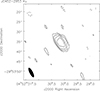 |
Fig. 1. Radio map of J0452-2953 at 15 GHz. The map rms is σ = 17 μJy, the contours are at [−3, 3, 6, 12, 24] ×σ. |
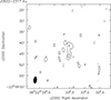 |
Fig. 2. Radio map of J0622-2317 at 15 GHz. The map rms is σ = 12 μJy, the contours are at [−3, 3, 6] ×σ. |
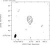 |
Fig. 3. Radio map of J1032-2707 at 15 GHz. The map rms is σ = 22 μJy, the contours are at [−3, 3, 6, 12, 18] ×σ. |
In J0452-2953, we can see elongated emission ∼23° in the south-east direction, which extends for ∼3″, that is ∼13 kpc in projected size. The same feature is visible at 22 and 33 GHz. For this reason, we decided to fit the source with two Gaussians, the first one representing the core, and the second the one-sided extended emission. We did the same for all the frequencies, and for both observing epochs (MJD 59872 and 59882). The results are reported in Table 1. The observations were taken ten days apart, and the integrated flux of the core and its spectral index remain constant over this interval. The steepness of the emission in the core may indicate that it originates from star formation in the nucleus, although it is possible that nuclear outflows are partially responsible for this emission. It is worth noting that the optical image of the galaxy, shown in Fig. 4, appears to be significantly elongated. Indeed, at a closer inspection, the galaxy shows two emission peaks 1.95″ apart in the Pan-STARRS image (8.4 kpc assuming that they are at the same distance), likely indicating that it is an interacting system. The radio emission seems to be associated with the south-east component.
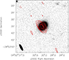 |
Fig. 4. In red the contours of J0452-2953 as in Fig. 1, overlapped with the i-band image of its host galaxy extracted from Pan-STARRS. |
Multi-epoch measurements of sources with extended morphology.
Parameters of linear and parabolic best fit for sources.
The extended flux instead seemingly shows some fast variability, especially at 15 and 22 GHz, and an inverted spectrum. Given the faintness of the emission, it is possible that the variability is only due to a non-perfect 2D fitting of the component, as it is highly unlikely to observe fast variability on a kpc-scale emission. Regarding the inverted spectrum, it may suggest the extended emission could originate in relativistic jets interacting with the interstellar medium (ISM), where the electrons are re-accelerated by this interaction. A similar behavior has already been observed in a couple more jetted NLS1s (Järvelä et al. 2022; Vietri et al. 2022), and can in principle affect also the optical emission lines (Hon et al. 2023; Dalla Barba et al. 2025). It is worth noting that the axis of the radio emission and that of the two nuclei are closely aligned, suggesting a possible connection between the two phenomena, although we cannot rule out that this is merely a projection effect. Deeper observations are needed to reach more precise conclusions on the nature of this object.
The source J0622-2317 was observed on MJD 59898 and 59899, but it was detected only at 15 GHz on the first date. The morphology is extended in the South direction for ∼6.5″ (∼4.8 kpc), and it also shows significant diffuse emission which cannot be fitted with two Gaussian components. The source was already observed by Chen et al. (2020), who only found a point-like compact morphology at 5 GHz with the JVLA. Such a spread-out morphology may originate from star formation. The spiral morphology of the host, shown in Fig. 5, is also supporting this hypothesis, as star formation activity could be ongoing both in the nucleus and in the spiral arms. Its integrated luminosity, calculated on the 3σ contour of the map, is rather low at log L = 37.95 ± 0.06 erg s−1, and it also supports the star formation origin of the radio.
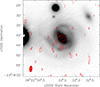 |
Fig. 5. In red the contours of J0622-2317 as in Fig. 2, overlapped with the i-band image of its host galaxy extracted from Pan-STARRS. |
Finally, we analyzed J1032-2707, whose 15-GHz map is shown in Fig. 3. The source was observed twice, on MJD 59862 and MJD 59903. In the first observation, the object clearly shows a double component at 15 GHz, as it does at 22 GHz, while at 33 GHz it was not detected. The emission at 15 GHz is extended for ∼5.2″ (∼7.1 kpc of projected size) approximately 33° North-East of the core. The two-point spectral index for the component corresponding to the optical nucleus is −0.85 ± 0.82, while the other component has a spectral index of −1.23 ± 0.78. Both were calculated using the integrated flux of the two Gaussian components. On the second observation, unfortunately, the beam is aligned almost exactly with the extended emission, and it is therefore preventing us from separating the two components and calculating two separate spectral indexes. It is worth noting that the extended emission is, at both frequencies, brighter than the core, with integrated luminosity at 15 GHz of log L = 39.08 ± 0.05 erg s−1, compared to 38.89 ± 0.05 erg s−1 for the core. Its spectral index is rather steep, and it is not clear if this emission corresponds to a relativistic jet, or if it is due to intense star formation, although the latter seems exceedingly bright at these frequencies.
3.2. Spectral shape
Out of 26 objects, three do not have enough data to properly fit their spectrum. J0413-0050 was detected only at two frequencies. We calculate that its two-point spectral index of the peak flux density of this source is −0.42 ± 0.13, that is between a flat- and a steep-spectrum source (threshold −0.5, see Foschini et al. 2015). J2244-1822 and J2358-1029 have only been detected at 15 GHz by the JVLA, suggesting that their spectral index is negative.
In four cases, the spectrum can be better reproduced with a log parabola. As previously mentioned, this could potentially suggest the presence of a curvature, which in turn could indicate some form of absorption, possibly SSA, at low frequencies. This feature could indicate the presence of a young relativistic jet, whose spectra indeed are peaked (Fanti et al. 1995). We tried to extrapolate the position of the peak in the spectrum. Two of them peak in the MHz range, while the other two peak in the kHz range. However, it is worth noting that only in one source, J0447-0508, the peak position is relatively well constrained, while for the others, the uncertainty is large. Let us assume that the spectral peak is related to the jet size, as described in Eq. (4) of O’Dea (1998). If this is the case, the sources peaking in the kHz range would have a jet of Mpc scale, which is not seen at any frequency or scale. Only in the case of J0447-0508 the peak frequency would correspond to a jet possibly confined within the host galaxy, ∼2.97 kpc. However, the scale for this source is 0.846 kpc/″. The corresponding linear size for a 90° inclination would be 3.5″ on the sky, but it could be smaller if the jet had a lower inclination. No sign of extended emission is visible in our maps. Therefore, either there is a jet with a rather small inclination, but we would then start seeing effects from relativistic beaming such as significant variability. Otherwise, the spectral curvature, if at all there, does not seem to imply that a jet is present.
One source is particularly interesting, J0239-1118. The source was detected by Chen et al. (2020) at 5 GHz, showing no particular features, but the high frequency observations revealed a strongly inverted spectrum, with αν = 0.28 ± 0.04. The peak of the emission is therefore at higher frequencies, and due to the lack of data, we could not constrain its position. In principle, an inverted spectrum at high frequency can originate from free–free absorption (FFA, Condon 1992). However, its spectral index in this case is expected to be much more inverted than what we observe, and on average, more inverted than SSA. Therefore, we suggest that this source is a high-frequency peaker (HFP, Orienti 2009), that is, a newborn relativistic jet growing quickly.
Another object in the sample, J0203-1247, has a spectral index of −0.35 ± 0.05, consistent with a classification as a flat-spectrum object. Its luminosity at 5 GHz was already calculated by Chen et al. (2020), who reported a value of 1.3 × 1038 erg s−1. This is much lower compared to the typical value of jetted NLS1s (Berton et al. 2018), therefore, the origin of this emission in this case may reside in a non-relativistic outflow produced by the nucleus, and not a relativistic jet.
Finally, the remaining 18 objects all show a negative slope, with values ranging between −0.5 and −0.94. These numbers, along with their point-like morphology in all of our observations, are all consistent with optically thin synchrotron emission. Its origin could be a jet, as is likely in J0452-2953, or from outflows, a jet base, or star formation.
3.3. Radio luminosity
We calculated the radio luminosity from the flux densities reported in Table A.2, following
 (1)
(1)
where DL is the luminosity distance, z the source’s redshift, and α is the spectral index, defined as Sν ∝ να. The spectral index was calculated directly on the data using the nearest frequency point. When this was not possible, for example, for upper limits, we used α = −1. We report all the luminosities in Table A.5, available online. In Berton et al. (2018), all the sources which most likely harbor a relativistic jet had a luminosity larger than 1040 erg s−1 at 5 GHz. Assuming the typical spectral index of synchrotron radiation, i.e. −0.7, this corresponds to a logarithmic luminosity of 39.67, 39.56, and 39.44 at 15, 22, and 33 GHz, respectively. Six of our sources exceed these thresholds in at least one frequency. This could suggest the presence of jets in these sources, but it is not so straightforward since strong star formation can also reach similar luminosities (Caccianiga et al. 2015). Finally, we checked for significant variability among sources with multiple observations. However, we did not find anything above 3σ, only some marginal differences at most within 2σ.
4. Discussion
4.1. The high frequency spectrum of NLS1s
In most sources, the main contribution to the radio emission probably comes from the active nucleus itself, that is, the synchrotron emission produced by non-relativistic outflows, or perhaps by the intense circumnuclear star formation that is often seen in NLS1s (Sani et al. 2010; Winkel et al. 2022, 2023). In principle, radio emission can also be produced by the accretion disk corona, but that typically produces a flat spectrum that we do not observe here (Raginski & Laor 2016). The accretion disk itself could be contributing to the radio spectrum by means of synchrotron or free-free emission (Abramowicz & Fragile 2013). Free–free emission, in particular, could be detectable at high radio frequency, with a characteristic slope of αν = 0.1 (Condon 1992). However, our spectral indexes are typically steeper than that, and are more indicative of synchrotron emission. Furthermore, the peak of the accretion disk usually falls in the ultraviolet band (e.g., Czerny & Elvis 1987; Panda et al. 2018; Ferland et al. 2020; Garnica et al. 2025), so if the disk contribution is present in our observations it is probably rather small. Other potential sources of steep-spectrum radio emission are a jet base (e.g., Giroletti & Panessa 2009), failed relativistic jets (Ghisellini et al. 2004), or fully developed small-scale relativistic jets seen at large angles. However, when we compare their luminosity to the sources studied by Berton et al. (2018), our objects are within the typical range of nonjetted sources, although we cannot completely rule out the presence of relativistic jets in them. For example, in J1032-2707 the luminosity is rather low, around 1039 erg s−1, but its morphology shown in Fig. 3 is reminiscent of a core-jet system. It is possible that this extended emission is a non-relativistic outflow, but only additional observations could confirm this scenario.
It is also worth noting that in our sources we do not see the so-called high-frequency excess (HFE) observed by Antonucci & Barvainis (1988) and Barvainis et al. (1996). With early VLA observations, they showed that several radio-quiet quasars or luminous Seyfert galaxies showed a steep spectrum at low frequencies (below 10 GHz), that turned flat or inverted above this frequency. Some objects showed an excess at even higher frequency (95 GHz), suggesting that the corona is responsible for this emission (Behar et al. 2015), although this point is still debated (Doi & Inoue 2016). A similar behavior was also observed in low-luminosity AGN, and in that case, the nature of the inverted spectrum was attributed to an advection-dominated accretion flow (Doi et al. 2005). Interestingly, some of the sources studied by Behar et al. (2015) are well-known NLS1s (Ark 564, Mrk 766, and also NGC 5506, the first obscured NLS1 ever discovered Nagar et al. 2002). This suggests the presence of diverse properties within the NLS1 class, which remain to be understood.
Finally, these radio spectra do not seem to be strongly variable, which is also consistent with the outflow scenario. In particular, we do not observe any sign of the extreme variability detected by MRO at 37 GHz and by OVRO at 15 GHz (Lähteenmäki et al. 2018; Järvelä et al. 2024). However, it is worth noting that the timescale for this new type of variability could be shorter than the cadence between our observations. Already in Järvelä et al. (2024) they found that the e-folding time of these flares can be as fast as one day, but more recent observations indicate that it could be even shorter (Crepaldi et al., in prep., Järvelä et al., in prep.). Therefore, it is not very surprising that the JVLA did not catch any of these flaring events. With our current knowledge, only dedicated monitoring at high frequency could find new examples of this intriguing phenomenon.
4.2. Potential new jetted NLS1s
It is evident from our work and that of many others (Berton et al. 2018; Chen et al. 2020, 2022, 2023; Järvelä et al. 2022) that identifying the nature of the radio emission in NLS1s is extremely challenging. Spectral indexes and morphology provide some indication, but do not paint the whole picture. Multiwavelength and multiscale observations are necessary to give more precise indications on the nature of these sources. It is also worth noting that our data, taken at 15, 22, and 33 GHz with the JVLA C configuration, can only study relatively small spatial scales, i.e. a few kpc. Some recent studies showed that some relativistic jets in NLS1 can have a very large size (Rakshit et al. 2018; Vietri et al. 2022; Chen et al. 2024), and can therefore be resolved out at the spatial resolution we are currently observing (Umayal et al. 2025). This, however, should not be the case for our objects, since the low-frequency points do not show any flux excess suggestive of extended emission.
However, with this work, we likely identified two new jetted NLS1s, J0239-1118, and J0452-2953. The latter is the most luminous source in our sample, with an integrated luminosity at 33 GHz of ∼5 × 1040 erg s−1, comparable to that of other known jetted NLS1s (Berton et al. 2018). It also shows an elongated emission that extends for 13 kpc in projected size toward south-east with an inverted spectrum. We attribute these properties to a possible relativistic jet interacting with the ISM. As shown in Fig. 4, the radio emission seems almost entirely confined within the host galaxy, so jet/ISM interaction is definitely possible, although this alignment may be coincidental and due just to projection effects. Other possible explanations for the inverted spectrum are forms of absorption, FFA or SSA, but they appear less likely at such a distance from the nuclear region. If the emission is due to a relativistic jet, considering its projected size as a lower limit and assuming a propagation velocity of ∼0.5c (Giroletti & Polatidis 2009), its age should be > 7.8 × 10⁴ years, within the typical range for NLS1s (Czerny et al. 2009).
As for J0239-1118, as we already mentioned, it could be an HFP. These objects belong to the larger class of peaked sources (PS, O’Dea & Saikia 2021), which is a mixed bag of different objects sharing one common observational property, that is, a peaked radio spectrum. The peak is due to significant SSA toward lower frequencies, which indicates that PS are typically small-scale relativistic jets still confined within their host galaxy. The PS class includes a number of frustrated jets that are not powerful enough to escape their host. At the same time, it also includes genuinely young sources such as compact steep-spectrum sources (CSS), gigahertz-peaked sources (GPS), and HFPs, in which the small size of the jet corresponds to young age. Since there is an anticorrelation between the jet age and the peak frequency (O’Dea & Baum 1997), HFPs are the youngest among all jets, so young that their spectra evolve quickly on an observable timescale. We therefore expect to observe significant variability in J0239-1118 within the next few years, which will allow us to constrain the peak position and confirm its nature as a young relativistic jet.
The presence of such a young jet in an NLS1 should not come as a surprise. The first suggestion of a connection between NLS1s and PS came already in the early 2000s, when some authors noted that a jetted NLS1 presented a peaked spectrum (Oshlack et al. 2001; Schulz et al. 2016). In the following years, it was suggested that some PSs, in particular the class of low-luminosity compact sources (Kunert-Bajraszewska et al. 2010) may be part of the parent population of gamma-ray NLS1s, since their radio luminosity functions (Berton et al. 2016) and host galaxy properties (Vietri et al. 2024) match each other. Finding an HFP in an NLS1 strengthens this view, proving once again that part of the parent population of gamma-ray emitting NLS1s can indeed be found among PS (Berton et al. 2017; Berton & Järvelä 2021).
Sources like this may be relatively common at high redshift. Indeed, to form the massive seeds that we observe in the early Universe (Inayoshi et al. 2020), relativistic jets can be instrumental in draining angular momentum and allowing for super-Eddington accretion (e.g., Volonteri et al. 2021). Recently, one blazar was identified at the epoch of reionization (Bañados et al. 2025), implying that a number of parent population sources should exist. Assuming that these objects look like J0239-1118, we can extrapolate the expected flux density at 3.0 GHz, where, for example, VLASS is currently observing. Assuming a spectral index of αν = 0.28, and extrapolating at z = 6, the flux density would be 1.96 μJy, which is well below the detection limit of any present-day survey. This estimate shows why only a handful of misaligned jets have been identified at the epoch of reionization (Bañados et al. 2021; Endsley et al. 2023). However, these sources could become detectable with future instrumentation such as the Square Kilometre Array (SKA).
Last, it is worth mentioning the source J2021-2235, a.k.a. IRAS 20181-2244. This NLS1 is hosted by a late-type galaxy interacting with a satellite (Berton et al. 2019), and it was identified as a jetted object by Komossa et al. (2006). Based on its infrared emission, it seems to have a remarkably high star formation of 300 M⊙ yr−1, which is responsible for a very significant fraction of its radio emission (Caccianiga et al. 2015). Its relativistic jet appears unresolved in our data as it was at 5 GHz (Chen et al. 2020), implying that it is either resolved out, genuinely very small, or it has a small projected size due to a low inclination. It is worth noting that J2021-2235 is the second most luminous source in our sample (∼4 × 1040 erg s−1 integrated at 15 GHz), and this suggests that the jet contribution plays a significant role also at these frequencies, possibly due to some limited contribution of relativistic beaming if the viewing angle is small.
5. Conclusions
In this paper, we report on our new JVLA observations of a sample of 50 NLS1s at 15, 22, and 33 GHz. Approximately half of the sources, 26, were detected at least at one frequency. We studied their radio properties by adding available data from the literature. Their spectrum is almost always steep and can be reproduced by a power law. The emission possibly originates in radiation pressure-driven non-relativistic outflows or, less likely, in circumnuclear star formation. The origin of these seemingly common outflows may lie in the strong radiation pressure produced by the high accretion typical of NLS1s. A couple of sources may harbor small-scale relativistic jets, and one in particular may be a high-frequency peaker. It is possible that more relativistic jets are present, but we cannot confirm their presence with the available data. These results confirm the complexity and diverse nature of the NLS1 class. Additional multiwavelength studies are necessary to fully characterize these sources, and understand their role in the AGN life cycle.
Data availability
Tables A.3, A.4, and A.5 are available at the CDS via https://cdsarc.cds.unistra.fr/viz-bin/cat/J/A+A/708/A46. All the radio maps not shown in the paper are available at zenodo. The raw data are publicly available from the NRAO archive.
Acknowledgments
We thank the anonymous referee for constructive comments that helped improving the paper. The authors are grateful to Dr. Elisa Garro for useful discussion on the nature of young relativistic jets. M.B. and E.J. acknowledge the support of the ESO Chile Visitor Program. A.J.G. and C.P. acknowledge the ESO Science Support Discretionary Fund 2025. I.V. acknowledges the support of the Swedish Cultural Foundation in Finland and the financial support from the Visitor and Mobility program of the Finnish Centre for Astronomy with ESO (FINCA). S.P. is supported by the international Gemini Observatory, a program of NSF NOIRLab, which is managed by the Association of Universities for Research in Astronomy (AURA) under a cooperative agreement with the U.S. National Science Foundation, on behalf of the Gemini partnership of Argentina, Brazil, Canada, Chile, the Republic of Korea, and the United States of America. The National Radio Astronomy Observatory and Green Bank Observatory are facilities of the U.S. National Science Foundation operated under cooperative agreement by Associated Universities, Inc. This research has made use of the NASA/IPAC Extragalactic Database (NED), which is operated by the Jet Propulsion Laboratory, California Institute of Technology, under contract with the National Aeronautics and Space Administration. This research has made use of the SIMBAD database, operated at CDS, Strasbourg, France. This research has made use of the VizieR catalog access tool, CDS, Strasbourg, France. The National Radio Astronomy Observatory is a facility of the National Science Foundation operated under cooperative agreement by Associated Universities, Inc. This research has made use of the CIRADA cutout service at URL cutouts.cirada.ca, operated by the Canadian Initiative for Radio Astronomy Data Analysis (CIRADA). CIRADA is funded by a grant from the Canada Foundation for Innovation 2017 Innovation Fund (Project 35999), as well as by the Provinces of Ontario, British Columbia, Alberta, Manitoba and Quebec, in collaboration with the National Research Council of Canada, the US National Radio Astronomy Observatory and Australia’s Commonwealth Scientific and Industrial Research Organisation. The National Radio Astronomy Observatory is a facility of the National Science Foundation operated under cooperative agreement by Associated Universities, Inc. LOFAR data products were provided by the LOFAR Surveys Key Science project (LSKSP; https://lofar-surveys.org/) and were derived from observations with the International LOFAR Telescope (ILT). LOFAR (van Haarlem et al. 2013) is the Low Frequency Array designed and constructed by ASTRON. It has observing, data processing, and data storage facilities in several countries, which are owned by various parties (each with their own funding sources), and which are collectively operated by the ILT foundation under a joint scientific policy. The efforts of the LSKSP have benefited from funding from the European Research Council, NOVA, NWO, CNRS-INSU, the SURF Co-operative, the UK Science and Technology Funding Council and the Jülich Supercomputing Centre. The Pan-STARRS1 Surveys (PS1) and the PS1 public science archive have been made possible through contributions by the Institute for Astronomy, the University of Hawaii, the Pan-STARRS Project Office, the Max-Planck Society and its participating institutes, the Max Planck Institute for Astronomy, Heidelberg and the Max Planck Institute for Extraterrestrial Physics, Garching, The Johns Hopkins University, Durham University, the University of Edinburgh, the Queen’s University Belfast, the Harvard-Smithsonian Center for Astrophysics, the Las Cumbres Observatory Global Telescope Network Incorporated, the National Central University of Taiwan, the Space Telescope Science Institute, the National Aeronautics and Space Administration under Grant No. NNX08AR22G issued through the Planetary Science Division of the NASA Science Mission Directorate, the National Science Foundation Grant No. AST-1238877, the University of Maryland, Eotvos Lorand University (ELTE), the Los Alamos National Laboratory, and the Gordon and Betty Moore Foundation.
References
- Abdo, A. A., Ackermann, M., Ajello, M., et al. 2009, ApJ, 707, L142 [NASA ADS] [CrossRef] [Google Scholar]
- Abramowicz, M. A., & Fragile, P. C. 2013, Liv. Rev. Relat., 16, 1 [Google Scholar]
- Angelakis, E., Fuhrmann, L., Marchili, N., et al. 2015, A&A, 575, A55 [NASA ADS] [CrossRef] [EDP Sciences] [Google Scholar]
- Antonucci, R., & Barvainis, R. 1988, ApJ, 332, L13 [Google Scholar]
- Arsenov, N., Frey, S., Kovács, A., & Slavcheva-Mihova, L. 2025, ApJS, 280, 23 [Google Scholar]
- Bañados, E., Mazzucchelli, C., Momjian, E., et al. 2021, ApJ, 909, 80 [CrossRef] [Google Scholar]
- Bañados, E., Momjian, E., Connor, T., et al. 2025, Nat. Astron., 9, 293 [Google Scholar]
- Barvainis, R., Lonsdale, C., & Antonucci, R. 1996, AJ, 111, 1431 [Google Scholar]
- Becker, R. H., White, R. L., & Helfand, D. J. 1995, ApJ, 450, 559 [Google Scholar]
- Behar, E., Baldi, R. D., Laor, A., et al. 2015, MNRAS, 451, 517 [NASA ADS] [CrossRef] [Google Scholar]
- Berton, M., & Järvelä, E. 2021, Astron. Nachr., 342, 1066 [NASA ADS] [CrossRef] [Google Scholar]
- Berton, M., Caccianiga, A., Foschini, L., et al. 2016, A&A, 591, A98 [NASA ADS] [CrossRef] [EDP Sciences] [Google Scholar]
- Berton, M., Foschini, L., Caccianiga, A., et al. 2017, Front. Astron. Space Sci., 4, 8 [NASA ADS] [CrossRef] [Google Scholar]
- Berton, M., Congiu, E., Järvelä, E., et al. 2018, A&A, 614, A87 [NASA ADS] [CrossRef] [EDP Sciences] [Google Scholar]
- Berton, M., Congiu, E., Ciroi, S., et al. 2019, AJ, 157, 48 [NASA ADS] [CrossRef] [Google Scholar]
- Berton, M., Järvelä, E., Crepaldi, L., et al. 2020, A&A, 636, A64 [NASA ADS] [CrossRef] [EDP Sciences] [Google Scholar]
- Berton, M., Järvelä, E., Tortosa, A., & Mazzucchelli, C. 2025, Open J. Astrophys., submitted [arXiv:2509.03576] [Google Scholar]
- Boroson, T. A., & Green, R. F. 1992, ApJS, 80, 109 [Google Scholar]
- Caccianiga, A., Antón, S., Ballo, L., et al. 2015, MNRAS, 451, 1795 [NASA ADS] [CrossRef] [Google Scholar]
- Chen, S., Berton, M., La Mura, G., et al. 2018, A&A, 615, A167 [NASA ADS] [CrossRef] [EDP Sciences] [Google Scholar]
- Chen, S., Järvelä, E., Crepaldi, L., et al. 2020, MNRAS, 498, 1278 [NASA ADS] [CrossRef] [Google Scholar]
- Chen, S., Stevens, J. B., Edwards, P. G., et al. 2022, MNRAS, 512, 471 [Google Scholar]
- Chen, S., Laor, A., Behar, E., Baldi, R. D., & Gelfand, J. D. 2023, MNRAS, 525, 164 [Google Scholar]
- Chen, S., Kharb, P., Silpa, S., et al. 2024, ApJ, 963, 32 [NASA ADS] [CrossRef] [Google Scholar]
- Condon, J. J. 1992, ARA&A, 30, 575 [Google Scholar]
- Condon, J. J., Cotton, W. D., Greisen, E. W., et al. 1998, AJ, 115, 1693 [Google Scholar]
- Congiu, E., Berton, M., Giroletti, M., et al. 2017, A&A, 603, A32 [NASA ADS] [CrossRef] [EDP Sciences] [Google Scholar]
- Congiu, E., Kharb, P., Tarchi, A., et al. 2020, MNRAS, 499, 3149 [NASA ADS] [CrossRef] [Google Scholar]
- Cracco, V., Ciroi, S., Berton, M., et al. 2016, MNRAS, 462, 1256 [NASA ADS] [CrossRef] [Google Scholar]
- Crepaldi, L., Berton, M., Dalla Barba, B., et al. 2025, A&A, 696, A74 [NASA ADS] [CrossRef] [EDP Sciences] [Google Scholar]
- Czerny, B., & Elvis, M. 1987, ApJ, 321, 305 [NASA ADS] [CrossRef] [Google Scholar]
- Czerny, B., Siemiginowska, A., Janiuk, A., Nikiel-Wroczyński, B., & Stawarz, Ł. 2009, ApJ, 698, 840 [NASA ADS] [CrossRef] [Google Scholar]
- Dalla Barba, B., Berton, M., Foschini, L., et al. 2025, A&A, 698, A320 [NASA ADS] [CrossRef] [EDP Sciences] [Google Scholar]
- Doi, A., & Inoue, Y. 2016, PASJ, 68, 56 [Google Scholar]
- Doi, A., Kameno, S., Kohno, K., Nakanishi, K., & Inoue, M. 2005, MNRAS, 363, 692 [NASA ADS] [Google Scholar]
- Endsley, R., Stark, D. P., Lyu, J., et al. 2023, MNRAS, 520, 4609 [Google Scholar]
- Fanti, C., Fanti, R., Dallacasa, D., et al. 1995, A&A, 302, 317 [NASA ADS] [Google Scholar]
- Ferland, G. J., Done, C., Jin, C., Landt, H., & Ward, M. J. 2020, MNRAS, 494, 5917 [Google Scholar]
- Foschini, L. 2011, in Narrow-Line Seyfert 1 Galaxies and their Place in the Universe. Proc. of Science, Vol. NLS1, 24 [Google Scholar]
- Foschini, L., Berton, M., Caccianiga, A., et al. 2015, A&A, 575, A13 [NASA ADS] [CrossRef] [EDP Sciences] [Google Scholar]
- Fraix-Burnet, D., Marziani, P., D’Onofrio, M., & Dultzin, D. 2017, Front. Astron. Space Sci., 4, 1 [NASA ADS] [Google Scholar]
- Ganci, V., Marziani, P., D’Onofrio, M., et al. 2019, A&A, 630, A110 [NASA ADS] [CrossRef] [EDP Sciences] [Google Scholar]
- Garnica, K., Dultzin, D., Marziani, P., & Panda, S. 2025, MNRAS, 540, 3289 [Google Scholar]
- Ghisellini, G., Haardt, F., & Matt, G. 2004, A&A, 413, 535 [NASA ADS] [CrossRef] [EDP Sciences] [Google Scholar]
- Giroletti, M., & Panessa, F. 2009, ApJ, 706, L260 [NASA ADS] [CrossRef] [Google Scholar]
- Giroletti, M., & Polatidis, A. 2009, Astron. Nachr., 330, 193 [Google Scholar]
- Gloudemans, A. J., Duncan, K. J., Röttgering, H. J. A., et al. 2021, A&A, 656, A137 [NASA ADS] [CrossRef] [EDP Sciences] [Google Scholar]
- Goodrich, R. W. 1989, ApJ, 342, 224 [Google Scholar]
- Ho, L. C., & Peng, C. Y. 2001, ApJ, 555, 650 [Google Scholar]
- Hon, W., Berton, M., Sani, E., et al. 2023, A&A, 672, L14 [NASA ADS] [CrossRef] [EDP Sciences] [Google Scholar]
- Inayoshi, K., Visbal, E., & Haiman, Z. 2020, ARA&A, 58, 27 [NASA ADS] [CrossRef] [Google Scholar]
- Intema, H. T., Jagannathan, P., Mooley, K. P., & Frail, D. A. 2017, A&A, 598, A78 [NASA ADS] [CrossRef] [EDP Sciences] [Google Scholar]
- Järvelä, E., Lähteenmäki, A., Lietzen, H., et al. 2017, A&A, 606, A9 [NASA ADS] [CrossRef] [EDP Sciences] [Google Scholar]
- Järvelä, E., Lähteenmäki, A., & Berton, M. 2018, A&A, 619, A69 [NASA ADS] [CrossRef] [EDP Sciences] [Google Scholar]
- Järvelä, E., Berton, M., & Crepaldi, L. 2021, Front. Astron. Space Sci., 8, 147 [CrossRef] [Google Scholar]
- Järvelä, E., Dahale, R., Crepaldi, L., et al. 2022, A&A, 658, A12 [NASA ADS] [CrossRef] [EDP Sciences] [Google Scholar]
- Järvelä, E., Savolainen, T., Berton, M., et al. 2024, MNRAS, 532, 3069 [CrossRef] [Google Scholar]
- Jose, J., Rakshit, S., Panda, S., et al. 2024, MNRAS, 532, 3187 [Google Scholar]
- Kellermann, K. I., Sramek, R., Schmidt, M., Shaffer, D. B., & Green, R. 1989, AJ, 98, 1195 [Google Scholar]
- Komatsu, E., Smith, K. M., Dunkley, J., et al. 2011, ApJS, 192, 18 [Google Scholar]
- Komossa, S. 2018, Proceedings of Science, Revisiting Narrow-line Seyfert 1 Galaxies and Their Place in the Universe, 15 [Google Scholar]
- Komossa, S., Voges, W., Xu, D., et al. 2006, AJ, 132, 531 [NASA ADS] [CrossRef] [Google Scholar]
- Kunert-Bajraszewska, M., Gawroński, M. P., Labiano, A., & Siemiginowska, A. 2010, MNRAS, 408, 2261 [NASA ADS] [CrossRef] [Google Scholar]
- Lacy, M., Baum, S. A., Chandler, C. J., et al. 2020, PASP, 132, 035001 [Google Scholar]
- Lähteenmäki, A., Järvelä, E., Ramakrishnan, V., et al. 2018, A&A, 614, L1 [NASA ADS] [CrossRef] [EDP Sciences] [Google Scholar]
- Lister, M. 2018, in Revisiting Narrow-line Seyfert 1 Galaxies andtheir Place in the Universe. 9-13 April 2018. Padova Botanical Garden, 22 [Google Scholar]
- Lister, M. L., Aller, M. F., Aller, H. D., et al. 2016, AJ, 152, 12 [NASA ADS] [CrossRef] [Google Scholar]
- Maiolino, R., Risaliti, G., Signorini, M., et al. 2025, MNRAS, 538, 1921 [Google Scholar]
- Marziani, P., Sulentic, J. W., Zwitter, T., Dultzin-Hacyan, D., & Calvani, M. 2001, ApJ, 558, 553 [NASA ADS] [CrossRef] [Google Scholar]
- Marziani, P., Dultzin, D., Sulentic, J. W., et al. 2018, Front. Astron. Space Sci., 5, 6 [CrossRef] [Google Scholar]
- Marziani, P., Garnica Luna, K., Floris, A., et al. 2025, Universe, 11, 69 [Google Scholar]
- Mathur, S. 2000, MNRAS, 314, L17 [NASA ADS] [CrossRef] [Google Scholar]
- McConnell, D., Hale, C. L., Lenc, E., et al. 2020, PASA, 37, e048 [Google Scholar]
- Moran, E. C. 2000, New Astron. Rev., 44, 527 [Google Scholar]
- Murphy, T., Sadler, E. M., Ekers, R. D., et al. 2010, MNRAS, 402, 2403 [Google Scholar]
- Nagar, N. M., Oliva, E., Marconi, A., & Maiolino, R. 2002, A&A, 391, L21 [NASA ADS] [CrossRef] [EDP Sciences] [Google Scholar]
- O’Dea, C. P. 1998, PASP, 110, 493 [Google Scholar]
- O’Dea, C. P., & Baum, S. A. 1997, AJ, 113, 148 [CrossRef] [Google Scholar]
- O’Dea, C. P., & Saikia, D. J. 2021, A&ARv, 29, 3 [Google Scholar]
- Olguín-Iglesias, A., Kotilainen, J., & Chavushyan, V. 2020, MNRAS, 492, 1450 [Google Scholar]
- Orienti, M. 2009, Astron. Nachr., 330, 167 [Google Scholar]
- Oshlack, A. Y. K. N., Webster, R. L., & Whiting, M. T. 2001, ApJ, 558, 578 [NASA ADS] [CrossRef] [Google Scholar]
- Osterbrock, D. E., & Pogge, R. W. 1985, ApJ, 297, 166 [Google Scholar]
- Panda, S., Czerny, B., Adhikari, T. P., et al. 2018, ApJ, 866, 115 [CrossRef] [Google Scholar]
- Panda, S., Marziani, P., & Czerny, B. 2019, ApJ, 882, 79 [NASA ADS] [CrossRef] [Google Scholar]
- Panessa, F., Baldi, R. D., Laor, A., et al. 2019, Nat. Astron., 3, 387 [Google Scholar]
- Peterson, B. M. 2011, Narrow-Line Seyfert 1 Galaxies and their Place in the Universe, 32 [Google Scholar]
- Pogge, R. W. 2011, Narrow-Line Seyfert 1 Galaxies and their Place in the Universe, 2 [Google Scholar]
- Raginski, I., & Laor, A. 2016, MNRAS, 459, 2082 [CrossRef] [Google Scholar]
- Rakshit, S., Stalin, C. S., Hota, A., & Konar, C. 2018, ApJ, 869, 173 [CrossRef] [Google Scholar]
- Richards, J. L., & Lister, M. L. 2015, ApJ, 800, L8 [NASA ADS] [CrossRef] [Google Scholar]
- Romano, P., Lähteenmäki, A., Vercellone, S., et al. 2023, A&A, 673, A85 [NASA ADS] [CrossRef] [EDP Sciences] [Google Scholar]
- Sani, E., Lutz, D., Risaliti, G., et al. 2010, MNRAS, 403, 1246 [Google Scholar]
- Schulz, R., Kreikenbohm, A., Kadler, M., et al. 2016, A&A, 588, A146 [NASA ADS] [CrossRef] [EDP Sciences] [Google Scholar]
- Shao, X., Edwards, P. G., Stevens, J., et al. 2025, MNRAS, 536, 1344 [Google Scholar]
- Shimwell, T. W., Röttgering, H. J. A., Best, P. N., et al. 2017, A&A, 598, A104 [NASA ADS] [CrossRef] [EDP Sciences] [Google Scholar]
- Sulentic, J. W., Zwitter, T., Marziani, P., & Dultzin-Hacyan, D. 2000, ApJ, 536, L5 [Google Scholar]
- Umayal, S., Paliya, V. S., Saikia, D. J., et al. 2025, ApJ, 995, 125 [Google Scholar]
- van Haarlem, M. P., Wise, M. W., Gunst, A. W., et al. 2013, A&A, 556, A2 [NASA ADS] [CrossRef] [EDP Sciences] [Google Scholar]
- Varglund, I., Järvelä, E., Hardcastle, M. J., Varglund, S., & Lähteenmäki, A. 2025, A&A, 703, A202 [NASA ADS] [CrossRef] [EDP Sciences] [Google Scholar]
- Varglund, I., Järvelä, E., Ciroi, S., et al. 2023, A&A, 679, A32 [NASA ADS] [CrossRef] [EDP Sciences] [Google Scholar]
- Varglund, I., Järvelä, E., Lähteenmäki, A., et al. 2022, A&A, 668, A91 [NASA ADS] [CrossRef] [EDP Sciences] [Google Scholar]
- Vietri, A., Järvelä, E., Berton, M., et al. 2022, A&A, 662, A20 [NASA ADS] [CrossRef] [EDP Sciences] [Google Scholar]
- Vietri, A., Berton, M., Järvelä, E., et al. 2024, A&A, 689, A123 [NASA ADS] [CrossRef] [EDP Sciences] [Google Scholar]
- Volonteri, M., Habouzit, M., & Colpi, M. 2021, Nat. Rev. Phys., 3, 732 [NASA ADS] [CrossRef] [Google Scholar]
- Wang, A., An, T., Kellermann, K. I., et al. 2025, ApJ, 987, L26 [Google Scholar]
- White, S. V., Jarvis, M. J., Häußler, B., & Maddox, N. 2015, MNRAS, 448, 2665 [Google Scholar]
- Winkel, N., Husemann, B., Davis, T. A., et al. 2022, A&A, 663, A104 [NASA ADS] [CrossRef] [EDP Sciences] [Google Scholar]
- Winkel, N., Husemann, B., Singha, M., et al. 2023, A&A, 670, A3 [NASA ADS] [CrossRef] [EDP Sciences] [Google Scholar]
- Yuan, W., Zhou, H. Y., Komossa, S., et al. 2008, ApJ, 685, 801 [NASA ADS] [CrossRef] [Google Scholar]
Appendix A: Tables
Sample of NLS1s observed with the JVLA.
Measurements for all the sources detected at least at one frequency in one epoch.
Appendix B: Radio maps
In the following section, we include the radio maps of the sources that show some sign of extended emission, and the overlap between the 15 GHz image and the Pan-STARRS i-band image. For J0452-2953, the map at 15 GHz observed on MJD 59872 is shown in Fig. 1, while its host galaxy in Fig. 4. For J1032-2707, the map at 15 GHz observed on MJD 59862 is shown in Fig. 3.
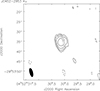 |
Fig. B.1. Radio map of J0452-2953 at 15 GHz, observed on MJD 59882. The map rms is σ = 17μJy, the contours are at [-3, 3, 6, 12, 24]×σ. |
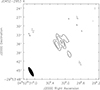 |
Fig. B.2. Radio map of J0452-2953 at 22 GHz, observed on MJD 59872. The map rms is σ = 30μJy, the contours are at [-3, 3, 6, 12]×σ. |
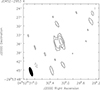 |
Fig. B.3. Radio map of J0452-2953 at 22 GHz, observed on MJD 59882. The map rms is σ = 26μJy, the contours are at [-3, 3, 6, 12]×σ. |
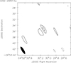 |
Fig. B.4. Radio map of J0452-2953 at 33 GHz. The map rms is σ = 39μJy, the contours are at [-3, 3, 6]×σ. |
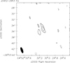 |
Fig. B.5. Radio map of J0452-2953 at 33 GHz. The map rms is σ = 36μJy, the contours are at [-3, 3, 6]×σ. |
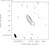 |
Fig. B.6. Radio map of J1032-2707 at 15 GHz, observed on MJD 59903. The map rms is σ = 15μJy, the contours are at [-3, 3, 6, 12, 24]×σ. |
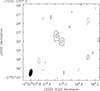 |
Fig. B.7. Radio map of J1032-2707 at 22 GHz, observed on MJD 59862. The map rms is σ = 35μJy, the contours are at [-3, 3, 6]×σ. |
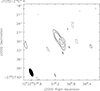 |
Fig. B.8. Radio map of J1032-2707 at 22 GHz, observed on MJD 59903. The map rms is σ = 22μJy, the contours are at [-3, 3, 6, 12]×σ. |
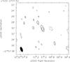 |
Fig. B.9. Radio map of J1032-2707 at 33 GHz, observed on MJD 59903. The map rms is σ = 30μJy, the contours are at [-3, 3, 6]×σ. |
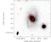 |
Fig. B.10. In red the contours of J1032-2707 as in Fig. 3, overlapped with the i-band image of its host galaxy extracted from Pan-STARRS. |
Appendix C: Radio spectra
All the radio spectra of the sources detected in at least one time at 15, 22, or 33 GHz with the JVLA. The symbols are as follows. The empty points indicate a flux density (left y axis), while solid points indicate integrated fluxes (right y axis). The red solid line shows the fit with a power law, while the blue dashed line is the fit with a log parabola. The empty triangles represent upper limits, calculated as three times the level of the noise in the images, and they are reported only for our new JVLA observations.
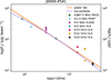 |
Fig. C.1. Spectrum of J0000-0541. Symbols as described in the text. |
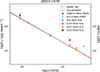 |
Fig. C.2. Spectrum of J0022-1039. Symbols as described in the text. |
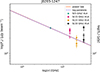 |
Fig. C.3. Spectrum of J0203-1247. Symbols as described in the text. |
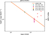 |
Fig. C.4. Spectrum of J0212-0201. Symbols as described in the text. |
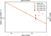 |
Fig. C.5. Spectrum of J0213-0551. Symbols as described in the text. |
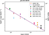 |
Fig. C.6. Spectrum of J0230-0859. Symbols as described in the text. |
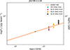 |
Fig. C.7. Spectrum of J0239-1118. Symbols as described in the text. |
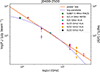 |
Fig. C.8. Spectrum of J0400-2500. Symbols as described in the text. |
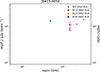 |
Fig. C.9. Spectrum of J0413-0050. Symbols as described in the text. |
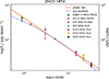 |
Fig. C.10. Spectrum of J0422-1854. Symbols as described in the text. |
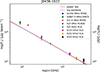 |
Fig. C.11. Spectrum of J0436-1022. Symbols as described in the text. |
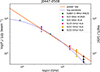 |
Fig. C.12. Spectrum of J0447-0508. Symbols as described in the text. |
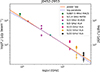 |
Fig. C.13. Spectrum of J0452-2953. Symbols as described in the text. |
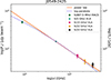 |
Fig. C.14. Spectrum of J0549-2425. Symbols as described in the text. |
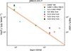 |
Fig. C.15. Spectrum of J0622-2317. Symbols as described in the text. |
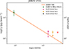 |
Fig. C.16. Spectrum of J0820-1741. Symbols as described in the text. |
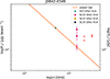 |
Fig. C.17. Spectrum of J0842-0349. Symbols as described in the text. |
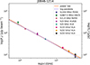 |
Fig. C.18. Spectrum of J0846-1214. Symbols as described in the text. |
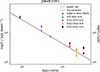 |
Fig. C.19. Spectrum of J0849-2351. Symbols as described in the text. |
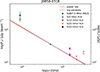 |
Fig. C.20. Spectrum of J0850-0318. Symbols as described in the text. |
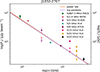 |
Fig. C.21. Spectrum of J1032-2707. Symbols as described in the text. |
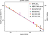 |
Fig. C.22. Spectrum of J1044-1826. Symbols as described in the text. |
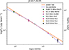 |
Fig. C.23. Spectrum of J1147-2145. Symbols as described in the text. |
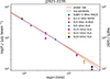 |
Fig. C.24. Spectrum of J2021-2235. Symbols as described in the text. |
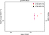 |
Fig. C.25. Spectrum of J2244-1822. Symbols as described in the text. |
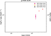 |
Fig. C.26. Spectrum of J2358-1029. Symbols as described in the text. |
All Tables
Measurements for all the sources detected at least at one frequency in one epoch.
All Figures
|
Fig. 1. Radio map of J0452-2953 at 15 GHz. The map rms is σ = 17 μJy, the contours are at [−3, 3, 6, 12, 24] ×σ. |
| In the text | |
|
Fig. 2. Radio map of J0622-2317 at 15 GHz. The map rms is σ = 12 μJy, the contours are at [−3, 3, 6] ×σ. |
| In the text | |
|
Fig. 3. Radio map of J1032-2707 at 15 GHz. The map rms is σ = 22 μJy, the contours are at [−3, 3, 6, 12, 18] ×σ. |
| In the text | |
|
Fig. 4. In red the contours of J0452-2953 as in Fig. 1, overlapped with the i-band image of its host galaxy extracted from Pan-STARRS. |
| In the text | |
|
Fig. 5. In red the contours of J0622-2317 as in Fig. 2, overlapped with the i-band image of its host galaxy extracted from Pan-STARRS. |
| In the text | |
|
Fig. B.1. Radio map of J0452-2953 at 15 GHz, observed on MJD 59882. The map rms is σ = 17μJy, the contours are at [-3, 3, 6, 12, 24]×σ. |
| In the text | |
|
Fig. B.2. Radio map of J0452-2953 at 22 GHz, observed on MJD 59872. The map rms is σ = 30μJy, the contours are at [-3, 3, 6, 12]×σ. |
| In the text | |
|
Fig. B.3. Radio map of J0452-2953 at 22 GHz, observed on MJD 59882. The map rms is σ = 26μJy, the contours are at [-3, 3, 6, 12]×σ. |
| In the text | |
|
Fig. B.4. Radio map of J0452-2953 at 33 GHz. The map rms is σ = 39μJy, the contours are at [-3, 3, 6]×σ. |
| In the text | |
|
Fig. B.5. Radio map of J0452-2953 at 33 GHz. The map rms is σ = 36μJy, the contours are at [-3, 3, 6]×σ. |
| In the text | |
|
Fig. B.6. Radio map of J1032-2707 at 15 GHz, observed on MJD 59903. The map rms is σ = 15μJy, the contours are at [-3, 3, 6, 12, 24]×σ. |
| In the text | |
|
Fig. B.7. Radio map of J1032-2707 at 22 GHz, observed on MJD 59862. The map rms is σ = 35μJy, the contours are at [-3, 3, 6]×σ. |
| In the text | |
|
Fig. B.8. Radio map of J1032-2707 at 22 GHz, observed on MJD 59903. The map rms is σ = 22μJy, the contours are at [-3, 3, 6, 12]×σ. |
| In the text | |
|
Fig. B.9. Radio map of J1032-2707 at 33 GHz, observed on MJD 59903. The map rms is σ = 30μJy, the contours are at [-3, 3, 6]×σ. |
| In the text | |
|
Fig. B.10. In red the contours of J1032-2707 as in Fig. 3, overlapped with the i-band image of its host galaxy extracted from Pan-STARRS. |
| In the text | |
|
Fig. C.1. Spectrum of J0000-0541. Symbols as described in the text. |
| In the text | |
|
Fig. C.2. Spectrum of J0022-1039. Symbols as described in the text. |
| In the text | |
|
Fig. C.3. Spectrum of J0203-1247. Symbols as described in the text. |
| In the text | |
|
Fig. C.4. Spectrum of J0212-0201. Symbols as described in the text. |
| In the text | |
|
Fig. C.5. Spectrum of J0213-0551. Symbols as described in the text. |
| In the text | |
|
Fig. C.6. Spectrum of J0230-0859. Symbols as described in the text. |
| In the text | |
|
Fig. C.7. Spectrum of J0239-1118. Symbols as described in the text. |
| In the text | |
|
Fig. C.8. Spectrum of J0400-2500. Symbols as described in the text. |
| In the text | |
|
Fig. C.9. Spectrum of J0413-0050. Symbols as described in the text. |
| In the text | |
|
Fig. C.10. Spectrum of J0422-1854. Symbols as described in the text. |
| In the text | |
|
Fig. C.11. Spectrum of J0436-1022. Symbols as described in the text. |
| In the text | |
|
Fig. C.12. Spectrum of J0447-0508. Symbols as described in the text. |
| In the text | |
|
Fig. C.13. Spectrum of J0452-2953. Symbols as described in the text. |
| In the text | |
|
Fig. C.14. Spectrum of J0549-2425. Symbols as described in the text. |
| In the text | |
|
Fig. C.15. Spectrum of J0622-2317. Symbols as described in the text. |
| In the text | |
|
Fig. C.16. Spectrum of J0820-1741. Symbols as described in the text. |
| In the text | |
|
Fig. C.17. Spectrum of J0842-0349. Symbols as described in the text. |
| In the text | |
|
Fig. C.18. Spectrum of J0846-1214. Symbols as described in the text. |
| In the text | |
|
Fig. C.19. Spectrum of J0849-2351. Symbols as described in the text. |
| In the text | |
|
Fig. C.20. Spectrum of J0850-0318. Symbols as described in the text. |
| In the text | |
|
Fig. C.21. Spectrum of J1032-2707. Symbols as described in the text. |
| In the text | |
|
Fig. C.22. Spectrum of J1044-1826. Symbols as described in the text. |
| In the text | |
|
Fig. C.23. Spectrum of J1147-2145. Symbols as described in the text. |
| In the text | |
|
Fig. C.24. Spectrum of J2021-2235. Symbols as described in the text. |
| In the text | |
|
Fig. C.25. Spectrum of J2244-1822. Symbols as described in the text. |
| In the text | |
|
Fig. C.26. Spectrum of J2358-1029. Symbols as described in the text. |
| In the text | |
Current usage metrics show cumulative count of Article Views (full-text article views including HTML views, PDF and ePub downloads, according to the available data) and Abstracts Views on Vision4Press platform.
Data correspond to usage on the plateform after 2015. The current usage metrics is available 48-96 hours after online publication and is updated daily on week days.
Initial download of the metrics may take a while.