| Issue |
A&A
Volume 708, April 2026
|
|
|---|---|---|
| Article Number | A288 | |
| Number of page(s) | 14 | |
| Section | Galactic structure, stellar clusters and populations | |
| DOI | https://doi.org/10.1051/0004-6361/202558728 | |
| Published online | 15 April 2026 | |
Revisiting the Milky Way stellar long bar and the 3 kpc arm★
1
Instituto de Astrofísica de Canarias,
38205
La Laguna,
Tenerife,
Spain
2
Departamento de Astrofísica, Universidad de La Laguna,
38206
La Laguna, Tenerife,
Spain
3
Institute of Astronomy and Physics, Inner Mongolia University,
Hohhot
010021,
China
4
National Astronomical Observatories, Chinese Academy of Sciences,
Beijing
100101,
China
5
Local Universe and Time-Domain Astronomy Laboratory, China West Normal University,
Nanchong
637002,
China
6
Luoxiahong Institute of Astronomy, China West Normal University,
Nanchong
637002,
China
7
Department of Astronomy, China West Normal University,
Nanchong
637002,
China
★★ Corresponding author: This email address is being protected from spambots. You need JavaScript enabled to view it.
Received:
22
December
2025
Accepted:
10
March
2026
Abstract
Context. One of the most difficult and unexplored regions of the Milky Way is the highly extincted in-plane central region within the Galactic coordinates 10◦ ≲ |ℓ| ≲ 30◦, |b| ≲ 3◦, where we have the long-bar and 3 kpc arm with intermediate-age stellar population, whose morphological properties are still unclear.
Aims. We aim to advance our knowledge of the morphology of these two components.
Methods. We examined star counts of bright M giants in WISE-4.6 µm and its distribution of distances derived from spectroscopic parallaxes with APOGEE-DR17. We also examined the distribution of distances of young OGLE-O-rich Mira variable stars, and reviewed the literature on red clump distance determination within that area.
Results. We corroborate the asymmetry between positive and negative longitudes in in-plane regions, thus confirming the necessity to include a long bar. We obtain an average angle between the major axis of the long bar and the line Sun–Galactic centre of α = 27.4◦ ± 1.5◦, aligned with the triaxial bulge and a semi-major-axis length ≈4 kpc. The tips of the long bar are in contact with the elliptical 3 kpc arm, with the major axis again aligned with the bulge and the long bar’s major axes, whose tangential lines of sight correspond to ℓ = −22◦ and ℓ = +27◦. In the range of 50 degrees in the sky between these two longitudes, the stellar near 3 kpc arm is clearly detected at heliocentric distances around 5 kpc, and the stellar far 3 kpc arm is tentatively detected at heliocentric distances of 9–12 kpc.
Key words: Galaxy: stellar content / Galaxy: structure
In memoriam of Terence J. Mahoney. The authors dedicate this paper to the memory of our late colleague, Terence J. Mahoney (1949–2025), who worked with some of us (MLC and FGL) over the last 30 years on analyses of the long bar within the Two-Micron Galactic Survey (TMGS) team (Tenerife, Spain).
© The Authors 2026
 Open Access article, published by EDP Sciences, under the terms of the Creative Commons Attribution License (https://creativecommons.org/licenses/by/4.0), which permits unrestricted use, distribution, and reproduction in any medium, provided the original work is properly cited.
This article is published in open access under the Subscribe to Open model. This email address is being protected from spambots. You need JavaScript enabled to view it. to support open access publication.
1 Introduction
One of the most difficult and unexplored regions of the Milky Way is the in-plane central region, namely within the Galactic coordinates |ℓ| ≲ 30◦, |b| ≲ 3◦. On the one hand, the extinction of the stars within central volume is high. On the other hand, the complexity of the Galactic structure is high, with several components to disentangle, which makes it difficult to analyse given that we observe them edge-on. For the stellar populations, apart from the stellar halo and disc and spiral arms, we have a triaxial bulge (dominant within |ℓ| ≲ 10◦) and other components necessary to explain the observed asymmetry of the star counts within 10◦ ≲ |ℓ| ≲ 30◦. Two major components have been identified for the stellar in-plane central regions so far: the long bar and the 3 kpc arm (or inner ring).
Dame et al. (1986) pointed out the existence of a large-scale long bar in the CO map whose tip is at the beginning of the Scutum arm. A similar conclusion examining stars in the near-IR band was obtained by Hammersley et al. (1994), which is the origin of the hypothesis of a stellar long bar. Its geometry was investigated either through the identification of the possible bar tips (López-Corredoira et al. 2001, 2007; González-Fernández et al. 2012; Amôres et al. 2013) or by measuring the distances of some of its stars, mainly with red clump stars (e.g. Hammersley et al. 2000; Benjamin et al. 2005; Cabrera-Lavers et al. 2008; Wegg et al. 2015, see further references and the discussion in Sect. 5) or other standard candles (e.g. van Loon et al. 2003). This long bar has stars younger (age ≲ 6 Gyr) than those of the bulge at a larger distance from the plane (Ng et al. 1996; Cole & Weinberg 2002; Nie et al. 2026) and metallicities that are disc-like or higher (González-Fernández et al. 2008; Wegg et al. 2019), which reveals either a peculiar wings-like extension of the bulge (a thicker structure; e.g. Martínez-Valpuesta & Gerhard 2011) or a structure different from the bulge with a different origin and/or evolution (López-Corredoira et al. 2011). In any case, the existence of a bulge and a long bar in a spiral galaxy is not surprising. There are also a few external galaxies that exhibit a bar and boxy bulge both visible photometrically (Sellwood & Wilkinson 1993; Bettoni & Galleta 1994; Compére et al. 2014) or with kinematical signatures in edge-on galaxies (Kuijken 1996).
One of the features of the long bar subject to dissensus is its orientation: it is claimed by some works to be the same as or very slightly larger than the triaxial bulge one (α between 20 and 30 degrees) or much larger by other authors. Using red clumps’ standard candles, Wegg et al. (2015) gave α = 28−33◦, where α is the angle between the major axis and the Sun–Galactic centre line, whereas much larger values were obtained with the red clumps by other works: α > 40◦ (e.g. Hammersley et al. 2000; Cabrera-Lavers et al. 2008). Using Gaia Data Release (DR) 2 data, Anders et al. (2019) gave an angle of the bulge+long bar of α ≈ 45 deg, with 30 million stars with photometry and parallaxes alone at |Z| < 3 kpc. It is dominated by the bulge in |ℓ| < 10◦ regions, but it includes in-plane regions for larger ℓ, showing the long bar with the angle of 45 deg. (Anders et al. 2019, Fig. 8). However, apart from the huge errors of the parallax for sources at distances larger than 5 kpc, Gaia wavelength is significantly affected by extinction, so it is not the most appropriate survey to study the long bar. Queiroz et al. (2021) considered that the angle of Anders et al. (2019) was overestimated because of extinction saturated over AV = 4 and the uses of parallaxes alone. Queiroz et al. (2021) used stars from Gaia DR2 and the Apache Point Observatory Galactic Evolution Experiment (APOGEE) DR16 with better distance determinations that have ∼10% errors and 0.2 kpc< |Z| <1 kpc, combined with other surveys, and obtained an angle value of ∼20 deg, though this was more focused in the bulge areas than the long-bar region. Anders et al. (2022) reconsidered the calculations with improved photo-astrometric distances and stellar density maps using Gaia Early DR3 data and multi-band photometry. Their StarHorse code includes a prior assumption of the orientation angle of the bulge and the long bar of 27◦, while their density map based on the red clumps suggests a bar angle that is a few degrees larger than the priors, especially near the tips of the long bar (Anders et al. 2022, Fig. 8). The analysis does not separate the bulge from the long bar, and it uses some priors, which makes it model dependent.
The question of the possible misalignment of the bulge and long bar remains unclear. Also, from the 3D decomposition of some galaxies with a long bar (e.g. NGC 3992), a significant misalignment between the long bar and the bulge of ∆α > 20◦ was claimed (Compére et al. 2014). Two triaxial structures (plus other components) with different angles is not theoretically impossible; they might be oscillating systems governed by a periodically time-dependent gravitational potential of variable length bars (Abramyan et al. 1986; Louis & Gerhard 1988; Garzón & López-Corredoira 2014), or their size ratio may be extreme, as in some double-barred galaxies (Shen & Debattista 2009). However, in most present-day models of bar formation, the two structures are presented as aligned or with only a slight twist near the tips due to an interaction with the adjacent spiral arm heads (see Martínez-Valpuesta & Gerhard 2011 and references therein), understanding the existence of a bulge and a long bar as different components of the same coherent bar structure as seen in simulations (Athanassoula 2005; Martínez-Valpuesta & Gerhard 2011; Li et al. 2015). Other dynamical aspects (e.g. Bland-Hawthorn & Gerhard 2016; Shen & Zheng 2020; Lucey et al. 2023; Hunt & Vasiliev 2025; Chen et al. 2025) have been associated with the features of the inner Galaxy, though most dynamical studies focus on the bulge (usually called the ‘bar’) and do not explicitly calculate the effect of this extension within the plane known as the ‘long bar’.
In the outskirts of the long-bar sweeping area, we find another structure called the 3 kpc arm. Historically, it was called the ‘arm’, though its nature is not related to the spiral arms. Rather than a spiral arm, the stars of the 3 kpc arm constitute an elliptical ring that delineates a trail of quasi-elliptical (X1) orbits around the Galactic bulge and long bar (Kumar et al. 2025). The 3 kpc arm structure appears likely to correspond to the radius of co-rotation resonance of the long bar (Green et al. 2011; Bland-Hawthorn & Gerhard 2016), with the long bar on its inner surface and the starting points of the spiral arms on its outer surface. The near part of the 3 kpc arm was discovered long time ago in HI (van Woerden et al. 1957), and CO evidence came later for the far 3 kpc arm behind the bulge and long bar (Dame & Thaddeus 2008). It includes young stars identified by maser emission (Green et al. 2011; Kumar et al. 2025) and a predominantly old stellar population, with an average age of ∼6 Gyr (Wylie et al. 2022); the vertical thickness of the ring decreases markedly towards younger ages (Wylie et al. 2022). There are red clump giants with high metallicity (Bland-Hawthorn & Gerhard 2016), and asymptotic giant branch stars (Churchwell et al. 2009). Dame & Thaddeus (2008) show that the 3 kpc arm contains a significant amount of molecular gas. The fact that this dense gas is not associated with strong tracers of recent star formation (such as HII regions; Lockman 1980) is a key piece of evidence in support of suppressed star formation in a region with a high concentration of gas, thus giving few or no OB main-sequence stars. It is likely due to the gas being highly turbulent and shocked by the Galactic bulge and long bar. The long bar gradually transitions into a radially thick, vertically thin, elongated inner ring with an average solar [Fe/H] (Wylie et al. 2022).
This stellar elliptical ring, called the 3 kpc arm, is so named because of its most prominent detection at ℓ = −22◦, b = 0 (Green et al. 2011; Davies et al. 2012), which corresponds to a tangential line of sight; assuming a Sun–Galactic centre distance of d ≈ 8 kpc gives R = d | sin(−22◦)| ≈ 3 kpc, though the radius is variable because it is not a perfect circular ring. Mikami et al. (1982) and Ruelas-Mayorga (1991) interpreted the ℓ = 27◦, b = 0 flux excess as the other tangential line of sight of the 3 kpc arm in positive longitudes, though ℓ = 27◦ was also interpreted as the possible tip of the long bar connecting to the Scutum spiral arm (Hammersley et al. 1994; López-Corredoira et al. 1999, 2001). This interpretational dissensus is also related to the angle, α, of the long bar, because a larger value of ℓ for the tip in the positive longitudes favours a larger α.
In this work, we aimed to shed further light on the morphology and nature of the long bar and 3 kpc arm. Section 2 of this paper describes how we used near- to mid-IR data of the Wide-field Infrared Survey Explorer (WISE; Wright et al. 2010) to show evidence of the asymmetry of star counts between the positive and the negative in-plane within 10◦ ≲ |ℓ| ≲ 30◦, which reinforces previous analyses even with a low extinction filter and even when a correction of extinction is included. In Sect. 3 we describe how we used spectroscopic parallaxes of APOGEE-2 (Majewski et al. 2017) data, with a distance accuracy of 10–20%, to derive the angle of the long bar. Section 4 outlines our use of Mira variable stars from the Optical Gravitational Lensing Experiment (OGLE) survey (Iwanek et al. 2022) with a relative distance precision of 4% to trace the structure of the long bar; we provide a new determination of its angle and the 3 kpc arm morphology. Section 5 features a reanalysis of the literature concerning the red clump’s relationship to the long bar and searches for the possible reasons of dissensus. Section 6 provides a summary and discussion of the results.
2 In-plane long-bar with WISE photometry
2.1 WISE data
The National Aeronautics and Space Administration (NASA)’s WISE (Wright et al. 2010) mapped the sky at 3.4, 4.6, 12, and 22 µm (W1, W2, W3, and W4) with an angular resolution of 6.1″, 6.4″, 6.5″, and 12.0″ in the four bands. According to the description on its web site, the AllWISE data (Cutri et al. 2014) we used here combine data from the WISE cryogenic and Near-Earth Object Wide-field Infrared Survey Explorer (NEO-WISE) (Mainzer et al. 2011) post-cryogenic survey phases to form the most comprehensive view of the full mid-IR sky currently available. By combining the data from two complete sky-coverage epochs using an advanced data-processing system, AllWISE generated new products that have enhanced photometric sensitivity and accuracy and improved astrometric precision compared to the 2012 WISE All-Sky Data Release. Exploiting the 6–12 month baseline between the WISE sky coverage epochs enables AllWISE to measure source motions for the first time and to compute improved flux-variability statistics. AllWISE contains accurate positions, apparent motion measurements, four-band fluxes, flux-variability statistics, and cross-correlations with Two-Micron All-Sky Survey (2MASS) sources (point-like and extended) for over 747 million objects detected on the co-added Atlas Images.
Photometry was performed using point-source profile-fitting and multi-aperture photometry. WISE 5σ photometric sensitivity is estimated to be at 16.6, 15.6, 11.3, and 8.0 Vega mag at 3.4, 4.6, 12, and 22 µm in unconfused regions on the ecliptic plane. Sensitivity is better at higher ecliptic latitudes where coverage is deeper and the zodiacal background is lower, and poorer when limited by confusion in high-source-density or complex-background regions. Saturation affects photometry for sources brighter than approximately 8.1, 6.7, 3.8, and −0.4 mag at 3.4, 4.6, 12, and 22 µm, respectively.
Here, we removed the extended sources (included in 2MASS-XSC extended-source catalogue), the sources with variability (flag ivafl1≥ 6) and those with a signal-to-noise ratio lower than 3. We limited our analysis to the Galactic coordinates |ℓ| < 40◦, |b| < 5◦: a total of 19 136 150 point-like sources, 612 417 of them with m4.6µm < 8.0.
These sources have associated J, H, and Ks magnitudes from cross-correlation with 2MASS. In 2MASS/J-filter, the limiting magnitude of completeness is 15.8 mag, reducing it to 14-15 mag in the crowded fields; this was expected in the plane of the galaxies. This means that we were limited to complete counts when (J − W2) ≲ 6 − 7, which may affect the loss of very reddened sources, but these are very few; for instance, of the 125 995 sources with m4.6µm < 8.0, |b| ≤ 0.5◦ (the in-plane region for the relevant analysis of the long bar) only 172 have no counterpart with all filters of 2MASS. The cross-correlation might have errors given the high crowdedness of these fields and the low angular resolution of WISE, but for very bright sources the number of in-plane sources is relatively low (around 2000 deg−2), and the probability of misidentification is low.
2.2 Asymmetry in star counts
In Fig. 1 we show the star counts within m4.6µm < 8.0. We clearly see an asymmetry within |b| < 0.5◦, with further counts for positive than negative longitudes within 5 ≲ |ℓ| ≲ 28◦. This asymmetry is gradually attenuated for larger values of |b|.
As said in the introduction, this asymmetry has been interpreted in terms of the existence of a new component of the Galaxy, namely long bar, which is different from the (thick) bar or bulge; it is also observable here and with its own asymmetry for off-plane regions. Previous analyses of this asymmetry (Hammersley et al. 1994; López-Corredoira et al. 2001, 2007; Wegg et al. 2015) have shown it in the K band, Galactic Legacy Infrared Midplane Survey Extraordinaire (GLIMPSE) 3.6µm, GLIMPSE 4.5µm, and the Midcourse Space Experiment (MSX) 8µm; here, we show the same trend with WISE 4.6 µm. Other bands of WISE show a similar trend (Fig. 1, bottom panel).
The 3 kpc arm (inner ring) without a long bar does not explain the in-plane features (Hammersley et al. 1994; López-Corredoira et al. 2001). A ring would be expected to produce a peak in the counts at the positions tangential to the line of sight: a U-shape rather than the monotonously increasing counts with ℓ within 10◦ ≲ ℓ ≲ 27◦. If the ring were elliptical, the longitudes of the peaks would no longer be symmetric; however, the shapes of the peaks would remain basically unaltered. It is possible that a contrived ring (particularly a patchy ring), coupled with a highly improbable distribution of extinction, could reproduce the form of the in-plane counts. However, as we show here, this distribution of extinction does not exist, and hence by itself the ring cannot explain the in-plane counts.
Extinction in 4.6 µm is very low: A4.6µm = 0.026AV = 0.33AK = 0.082E(B − V) = 0.158E(J − K) (Wang & Chen 2019). The application of an extinction correction cannot be carried out with a 3D extinction map, because we have no information on the distances of the sources here. The cumulative extinction cannot be applied for all stellar populations, because it affects the sources in the centre of the Galaxy behind the dust disc, but not nearby sources in the disc. Nonetheless, we can carry out an approximate correction for the extinction by means of
![Mathematical equation: $\matrix{ {{A_{4.6{\rm{\mu m}}(W2)}}(\ell ,b) = {{\left\langle {0.158[(J - K) - 1.1]} \right\rangle }_{\ell ,b,(J - K) > 1.0}}} \cr {{m_{4.6{\rm{\mu m}}(W2),0a}} \equiv {m_{4.6{\rm{\mu m}}}} - 0.158\,[(J - K) - 1.1];} \cr {{\rm{only for}}({\rm{J}} - {\rm{K}}) > 1.0.} \cr } $](/articles/aa/full_html/2026/04/aa58728-25/aa58728-25-eq1.png) (1)
(1)
The value of intrinsic colour, (J − K)0 = 1.1, is derived as the average colour (1.5) in regions within our selected area of low extinction; this is shown in Fig. 2 for (J − K) > 1.0 stars, with a correction of ⟨E(J − K)⟩ = 0.4 in this region (Schlegel et al. 1998). This intrinsic color (J − K)0 = 1.1 corresponds to M giants (Covey et al. 2007). Given the range of selected magnitudes (m4.6µm < 8.0), we are dominated by M giants at heliocentric distances of d =5–12 kpc, with some contamination of dwarfs and red clumps at d < 1 kpc from the disc. With the constraint (J − K) > 1.0, we removed most of the main-sequence stars and red clump giants of the disc (see Fig. 2). Different combinations of filters other than J and K are not as precise when it comes to the correct identification and separation of disc stars. We know this method is not perfect; as stated in Sect. 2.1, we lose some stars in very extincted regions which reach J > 14−15, but these are very few (negligible). We applied average extinction laws, which may have some fluctuations. Nonetheless, for our purpose, it is good enough.
Figure 3 gives the map of extinction-corrected star counts: m4.6µm,0a > 8.0, (J − K) > 1.0. We observe the same asymmetry of star counts in in-plane regions than in Fig. 1, though with much smaller fluctuations for both the bulge and the long bar. Figure 4 shows the extinction in 4.6µm, which is low, as expected: around 0.5 magnitudes on average within |b| < 0.5◦ and with a small dependence on the Galactic longitude. There is not an asymmetry in extinction between positive and negative Galactic longitudes, apart from fluctuations and a small tilt in the dependence with b at |ℓ| ≲ −15◦. Everything is in agreement with previous observations by López-Corredoira et al. (2001).
The conclusions are the same as those of Hammersley et al. (1994) and López-Corredoira et al. (2001, 2007): extinction cannot explain the asymmetry we observe in star counts. Neither the disc nor spiral arms can produce this asymmetry. Hence, there should be a structure of stars (here, we observe mainly M giants, but there are other populations) that are well constrained within the plane and have strong non-axisymmetry; these are in the long bar. The observed in-plane excess of stars located at ℓ ≈ −22◦ corresponds to a young massive star cluster (Green et al. 2011; Davies et al. 2012) and is thought to be a tangential cross of the 3 kpc arm (López-Corredoira et al. 2001).
The excess of star counts at positive longitudes with respect to negative longitudes for 15◦ < |ℓ| < 30◦ indicates that the closest part of the long bar is in the first quadrant. This asymmetry of star counts is observed even at |b| ≳ 3◦ (Fig. 3, middle panel), though the very fast decline of star counts with increasing latitude indicates that the structure is much more concentrated in the plane than the bulge (=thick bar; dominant at ℓ ≲ 10◦).
There is also a slight asymmetry in the vertical direction, with further star counts at negative latitudes than positive latitudes (Fig. 3, bottom panel). The star counts are vertically symmetrical with respect to b = −0.2◦ instead of b = 0. This small shift might be due some residuals of extinction correction, but it most likely has to do with the position of the Sun over the Galactic plane. A shift of z⊙ ∼ +20 pc over the plane (as observed; e.g. Karim et al. (2017) estimated that the Sun lies at z⊙ = 17 ± 5 pc above the Galactic mid-plane, and the median of 55 previous estimates published is z⊙ = 17 ± 2 pc) means that a structure at d ≈ 6 kpc is vertically shifted  with respect to b = 0.
These WISE stars have, on average, a corrected-for-extinction H-magnitude equal to H0 ≈ 7.5, which at distances of <5 kpc corresponds to absolute magnitudes of MH < −6.0, which again is in agreement with them being M giants (Covey et al. 2007). We see the distribution of distances to these M-giant stars in Sect. 3.
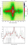 |
Fig. 1 WISE star counts. Top: as a function of ℓ, b within |ℓ| < 40◦, |b| < 5◦, m4.6µm < 8.0, ∆ℓ = 1◦, ∆b = 0.1◦. Bottom: as a function of ℓ within |ℓ| < 40◦, |b| < 0.5◦, for m3.4µm < 8.2, m4.6µm < 8.0, m12µm < 7.0, m22µm < 4.5, ∆ℓ = 1◦. |
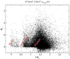 |
Fig. 2 Colour-magnitude diagram in low extincted areas (30◦ < |ℓ| < 40◦, 4◦ < |b| < 5◦; ⟨E(J − K)⟩ = 0.4; Schlegel et al. 1998) for sources with m4.6µm < 8.0. |
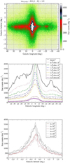 |
Fig. 3 WISE star counts as in Fig. 1 (top panel) but with stars with J − K < 1.0 removed (dwarfs and red clumps from Galactic disc) and with the correction of extinction through Eq. (1). We observe a prominent asymmetry between positive and negative Galactic longitudes and a very slight asymmetry between positive and negative Galactic latitudes. |
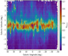 |
Fig. 4 Extinction A4.6µm as a function of ℓ, b within |ℓ| < 40◦, |b| < 5◦; ∆ℓ = 1◦, ∆b = 0.1◦, derived from Eq. (1). |
2.3 Angle of the long bar
In the first quadrant, the tip of the long bar is typically situated at ℓ = 27◦ − 30◦ (López-Corredoira et al. 1999, 2001, 2007; Zhang et al. 2014). Here, we also see a fast drop of counts at exactly ℓ = 27◦ in Fig. 1 (bottom panel), in agreement with that idea. However, ℓ = 27◦ might instead be a peak due to the tangential cut of the 3 kpc arm (Mikami et al. 1982; Ruelas-Mayorga 1991), and the tip of the long bar would be placed in a lower Galactic longitude. Examining the continuity of the excess of stars in the in-plane region with ℓ > 0, a more conservative position for the tip of the long bar in the positive longitudes would be ℓ1 = 27◦ ± 3◦, given that we also observe a significant drop of stars at ℓ = 24◦ even after extinction correction (Fig. 3, top panel) and that the region of excess stars might extend up to ℓ ≈ 30◦.
Conversely, in the negative longitudes, the terminus of the long bar is located between ℓ = −12◦ and ℓ = −14◦ (López-Corredoira et al. 2001; González-Fernández et al. 2012; Amôres et al. 2013). Here,in examining the extinction-corrected star counts of Fig. 3 (top), we would place the limits as ℓ2 = −12◦ ± 2◦.
Given these data, with a projection of the long bar, we can derive the angle of the bar (α) with respect to Sun–Galactic centre’s line of sight. In fact, it is a simple trigonometrical problem if we take the bar to be rectilinear and of equal length (L0) from each end to the centre (López-Corredoira et al. 1999):
 (2)
where R⊙ is the Sun–Galactic centre distance. Hence,
(2)
where R⊙ is the Sun–Galactic centre distance. Hence,
 (3)
(3)
(independent of R⊙). With the above values of ℓ1 and ℓ2, we obtain
 (4)
(4)
3 In-plane long bar with APOGEE-2 spectroscopy
3.1 APOGEE-2 data
We used the Sloan Digital Sky Survey Data fourth-phase (SDSS-IV) DR17 (Abdurro’uf et al. 2022) as a source for the following: the H-band (1.51–1.70 µm) high-resolution (R ∼ 22 500) spectra of the APOGEE-2 survey, with distances derived by Stone-Martínez et al. (2024) for 733 901 independent sources with near-IR spectra using neural networks with uncertainties of 10–20%. The data include northern- and southern-hemisphere observations from two different telescopes and spectrographs: APOGEE spectrograph on the 2.5 m Sloan Foundation Telescope at Apache Point Observatory (APO) in New Mexico, USA and an identical spectrograph on the 2.5 m Irénée du Pont Telescope at Las Campanas Observatory (LCO) in Chile. The Galactic disc is targeted with a more or less systematic grid of pointings within |b| < 15 deg. For 0 < ℓ < 30 deg., there is denser coverage of the bulge and inner Galaxy. It provides a statistically robust sample for studying the Galaxy, but it does not contain every star in its magnitude range.
The typical H-band magnitude range was ≈7 to ≈13.5. APOGEE-2’s primary sample is magnitude-limited (H < 12.2, or H < 12.8 in some bulge fields; using 2MASS photometry), but its completeness is heavily modified by a density-based selection algorithm (Zasowski et al. 2017). This means that while the pool of potential targets is all stars brighter than a certain H-band magnitude, not all of these stars are observed. The selection is designed to handle the immense stellar density, particularly toward the Galactic bulge and disc. APOGEE-2 does not randomly select all stars brighter than H=12.2. Instead, it uses a statistical sampling rate that varies with stellar density. In low-density fields (e.g. high Galactic latitude and halo), the sampling rate is 100%. In high-density fields (e.g. the Galactic plane and bulge), the probability of a star being selected is inversely proportional to the local stellar density. As a result, the completeness as a function of magnitude in a crowded sightline is nearly flat for bright magnitudes (e.g. from H=7.0 to H=12.2), but at a value of much less than 100%. The drop in completeness is not primarily due to magnitude, but to density on the sky. Furthermore, with the ‘Faint Time’ and Ancillary Science Samples, APOGEE-2 also included secondary targets, in the 12.2 < H < 13.5 range (sometimes even fainter for special programs like star clusters or dwarf galaxies). APOGEE-2’s main target selection also used colour cuts: (J − K)0 > 0.5 in disk and bulge areas, which means that the sources are mainly K or M spectral types, though there are also some sources with bluer colours.
We are only interested in the central in-plane areas of the Milky Way, so we added the following constraints: |ℓ| ≤ 40◦, |b| ≤ 5◦. Here, we select a subsample with the criteria −6.5 < MH < −5.5, 1.0 < (J − K)0 < 1.5 within a distance of 5 < d < 10 kpc and AH < 2.7; they correspond to 7.0 < H < 12.2, which is within the range of observed magnitudes, where there is flat completeness as a function of magnitude. This range of absolute magnitudes and colours corresponds to M5-6III (M giants) stellar types (Covey et al. 2007). In total, we have 1391 stars with these characteristics; see Fig. 5 (top panel). This selection of stars should contain a negligible amount of disc stars for distances larger than 12 kpc (M5-6 giants are too faint there) or lower than 4 kpc (they are too bright).
The deficit of stars in the innermost plane (|b| ≲ 1◦) is due to their higher extinction, with many stars having AH > 2.7. We should avoid regions with high extinction: not only should the average AH be much lower than 2.7 (equivalent to A4.6µm < 0.51 at Fig. 4), but also, due to the patchiness of the extinction, the ratio of stars with AH > 2.7 should be low (<5% of the stars at a distance between 5 and 10 kpc). This is followed for lines of sight of |b| > 1◦, so we apply this constraint in the following analyses.
3.2 Distribution of distances
With these APOGEE data, we do not see the asymmetry positive–negative longitudes as clearly as with WISE data because there are very few data with negative longitude in the in-plane regions. Furthermore, the scarcity of APOGEE sources is strongly concentrated at ℓ > 5, which makes the top panel of Fig. 5 rather incomplete. Nonetheless, APOGEE provides distances, whereas WISE does not, which allowed us to see a significant variation of heliocentric distances with Galactic longitude; the latter was used to determine the angle of the long bar with more precision than when only using the positions of the tips of the bar in WISE. The bottom panel of Fig. 5 contains a sufficient number of stars per bin to accurately determine the location of the density peak along each line of sight, thereby allowing the bar’s position angle to be reliably traced.
Figure 5 (bottom panel) shows the distribution of distances for −6◦ < ℓ < 30◦, 1◦ < |b| < 2.5◦ (a total of 1060 stars). The star density is calculated as  , where ω is the solid angle of each bin and N(r)dr is the star counts between r − dr/2 and r + dr/2. We chose this range of Galactic longitudes to trace the long bar, avoiding its far side because our sample does not reach the very distant stars in the negative Galactic longitudes. We avoided the areas of highest extinction with |b| < 1◦. On the other hand, |b| was restricted to the region where we find a significant presence of the long bar in the WISE survey.
Figure 5 (bottom panel) shows a continuous structure with a slightly decreasing distance for an increasing Galactic longitude. This indicates the presence of a barred structure up to ℓ = +26◦.
The dispersion of the distance values is of the order of the distance error; thus, the long bar should not be a thick structure. The average distance of the central stars (|ℓ| < 2◦) is 8.3 kpc. Note that the disk contribution in the central regions is not significantly detected; for instance, at |ℓ| < 5◦ we observe few stars with d < 5 kpc, and for 15◦ < ℓ < 30◦ we find very few stars with d > 10 kpc. There is not an axisymmetric structure in the central areas for these selected stars of Fig. 5 (bottom panel). Therefore, we neglected the contribution of the disk.
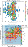 |
Fig. 5 Top: APOGEE-2/DR17 M5-6III (−6.5 < MH < −5.5, 1.0 < (J − K)0 < 1.5) star counts, in the range of Galactic coordinates |ℓ| < 40◦, |b| < 5◦. These counts are highly in incomplete (and white areas are unobserved regions) due to the observing strategy of APOGEE-2, but for each line of sight the completeness is constant, with a magnitude within 7.0 < H < 12.2 when AH < 2.7. Bottom: distribution of distances of these stars for −6◦ < ℓ < 30◦, 1.0◦ < |b| < 2.5◦; dashed line shows the best fit to a long bar with an angle of α = 25.6◦ for ℓ > 10◦. |
3.3 Angle of the long bar
Given that the APOGEE survey is highly incomplete, we were not able to build a 3D map of the density in the Galactic-bar region. A fit of the angle of the long bar in an incomplete 3D map would be very complex and subject to many uncertainties with regard to the selection function. Nonetheless, keeping in mind that for each line of sight the distribution of distances d between ≈5 and ≈10 kpc has the same level of completeness, a direct fit of the long-bar structure of d(ℓ) is possible. For each line of sight with a given ℓ, we crossed the long bar at a certain distance, dL, and the number of stars with measured d over and below dL should be similar. Assuming the long bar is a narrow structure and the maximum density of stars in the line of sight traces its major axis (see Appendix A of López-Corredoira et al. 2007), the distance of this structure in the in-plane regions is
 (5)
(5)
where α is the angle of the long bar with respect to the lines Sun–Galactic centre. We assumed R⊙ = 8.2 ± 0.2 kpc (from different measurements in the literature). We also assumed all of the stars in the line of sight are at the same distance. This approximation is not valid for a (thick) bulge, so the analysis of a triaxial bulge angle cannot be carried out with the same simplistic assumptions.
With our distribution of distances, d(ℓ), for the 167 stars with 10◦ < ℓ < 30◦ (we avoided the region dominated by the thick bulge) and 1.0◦ < |b| < 2.5◦ (we avoided the high-extinction areas and limited the maximum latitude where the asymmetry in WISE star counts is significant), a minimum χ2 analysis gives a value of α = 25.6◦ ± 2.3◦. The dashed line in the bottom of Fig. 5 shows this best fit. The errors in the fitting include global statistical errors and are due to the assumed error of R⊙. For 10◦ < ℓ < 24◦ (avoiding the thick bulge and possible confluence with the 3 kpc arm), 1.0◦ < |b| < 2.5◦: α = 25.5◦ ± 2.3◦ (165 stars).
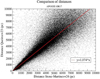 |
Fig. 6 Comparison of distances estimated for APOGEE-DR17 with the algorithms of Queiroz et al. (2023) and Stone-Martínez et al. (2024), respectively. |
3.4 With StarHorse distances
We used distances from Stone-Martínez et al. (2024) in APOGEE-DR17 stars. There is another estimation of distances of APOGEE-DR17 sources using the StarHorse algorithm (only for 562 424 stars; Queiroz et al. 2023), which gives an average of 7.4% larger distances for stars within a Stone-M.-distance of <10 kpc (see Fig. 6). From Eq. (5),  . For αStone−M. = 25.5◦, ⟨ℓ⟩ = 17◦, we obtain αStarHorse = 30.1◦.
4 In-plane long bar with OGLE Mira variable stars
4.1 OGLE data of Mira variable stars
The Iwanek et al. (2022) catalogue contains 65 981 Mira stars in the Milky Way based on the third and the fourth phases of the OGLE project. There are two subtypes: C-rich and O-rich. From the total, 40 356 stars are from bulge fields and 25 625 Miras are in disc fields. The authors provided light curves in the I and V bands from the Johnson–Cousins photometric system collected from 1996, December to 2020, March. The collection covers ∼3000 deg2 of the sky. The catalogue containing equatorial coordinates, pulsation periods (P), I-band brightness amplitudes, mean magnitudes in the V and I bands, light curves, and finding charts is publicly available and can be accessed through the OGLE Internet Archive1. The relative precision of the distance determination is around 4% (Catchpole et al. 2016). Cross-correlation with mid-IR data including WISE filters was added by Iwanek et al. (2023). Iwanek et al. (2023) limited their exploration space to a 3D cuboid: −4.2 kpc≤ X ≤3.8 kpc, −4 kpc≤ Y ≤4 kpc, and −2 kpc ≤ Z ≤ 2 kpc, with (X,Y,Z) Cartesian Galactic coordinates centred in the Galactic centre (R⊙ = 8.2 kpc) and thus covering the central parts of the Milky Way. This limit left us with 39 619 Miras, which are the ones used here.
In this section we restrict our analysis to the Miras within |ℓ| ≤ 40◦, |b| ≤ 5◦. We also removed C-rich Miras, as these stars usually change their mean brightness over time due to the significant mass-loss phenomenon (Iwanek et al. 2023). We are interested in the brightest and youngest population, which offer a better contrast between the long bar and the bulge, so we only selected stars with log10[P(days)] > 2.6; they correspond to M4.6µm < −8.5 (apparent W2 magnitude between 5.0 and 6.5 at distances between 5 and 10 kpc with negligible extinction; Iwanek et al. 2021) and ages <5 Gyr (Catchpole et al. 2016). With all of these criteria, there remains 10 581 O-rich Mira stars. Figure 7 (top panel) shows the star-count distribution as a function of Galactic coordinates.
The completeness of these sources is much lower than 100% in regions with high extinction (in I-filter), as indicated by Iwanek et al. (2023) with a mask. Outside the mask, in areas where completeness is almost 100%, there are 5371 O-rich Mira stars. Figure 7 (bottom panel) shows the star counts once the stars in the masked regions are removed. The comparison of masked and unmasked regions shows that we lose stars due to incompleteness even at |b| in the entire region, though predominantly at |b| < 1◦. The loss of stars of bins at higher latitudes is due to the existence of a few (not all) small areas with high extinction, even when the average extinction is not high due to the patchiness of the extinction.
4.2 Distribution of distances
In Fig. 8 (top panel) we show the distribution of distances for stars with a mask (removing the high-extinction areas) for 1.5◦ < |b| < 2.5◦, where the extinction is moderate on average. In Fig. 8 (bottom panel), we show the distribution of distances for stars with mask for |b| < 1.5◦, where the extinction is high, on average, and the completeness is low, except in a small portion of areas corresponding to holes of extinction.
The bulge area |ℓ| < 10◦ is well represented by the global angle of the major of the bulge. Iwanek et al. (2023) calculated an angle of the major axis of the bulge α = 20.1◦, and, although there should be some difference between the maximum star-count line and the major axis due to the thickness of the bulge (López-Corredoira et al. 2007, Appendix A), we see that this angle may also roughly represent the bulge region in near-plane regions. However, there is a prolongation between ℓ = 10◦ and ℓ = 30◦ that belongs to another structure with a different angle. The distance obtained at ℓ = 25−30◦ is around 5.5 kpc, which agrees with the value obtained by Zhang et al. (2014) of  kpc. This feature also resembles the distribution given by Wegg et al. (2015, Fig. 6) for red clump stars in the K band.
Given the incompleteness in some bins, especially at |b| < 1.5◦, the deficit of stars at some Galactic longitudes cannot be interpreted in terms of density drops. Nonetheless, since we used the stars outside the mask of low-incompleteness areas, the distribution of distance as a function of Galactic longitude should not be affected.
The shape of the isodensity contours might be interpreted as a long-bar detection at 10◦ ≲ ℓ ≲ 24◦, though with some deficit of stars due to incompleteness. The strong excess of stars at ℓ ≈ 24−30◦ corresponds to a well-known in-plane region where the star formation rate is high (López-Corredoira et al. 1999; Negueruela et al. 2010; Zhang et al. 2014), with a constant heliocentric distance of d ≈ 5.5 kpc; this is significantly deviated from the extrapolation of the bar at shorter wavelengths. This may indicate a structure that is not a straight bar, or easier to understand in terms of the fragment of the 3 kpc arm, which is tentatively the same one tangentially observed at ℓ ≈ −22◦, but at positive longitudes.
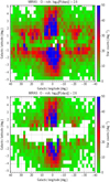 |
Fig. 7 Top: O-rich Mira variable star counts, with a period, P, within log10[P(days)] > 2.6, in the range of the Galactic coordinates |ℓ| < 40◦, |b| < 5◦. Bottom: same as the top panel but with the stars within the mask corresponding to regions of high extinction and low completeness removed (see Iwanek et al. 2023). |
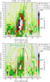 |
Fig. 8 Distribution of distances of O-rich Mira variable stars with a period, P, within log10[P(days)] > 2.6 for −20◦ < ℓ < 30◦, 1.5◦ < |b| < 2.5◦ (top panel; moderate extinction, high completeness) or |b| < 1.5◦ (bottom panel; high extinction, low completeness). The dashed line shows the best fit to a long bar within 10◦ < ℓ < 30◦ for bins with a mask (removing the high-extinction areas), d < R⊙, whereas the dotted line shows the corresponding d(ℓ) for an angle of α = 20.2◦, as fitted for the major axis of the bulge (Iwanek et al. 2023). The dashed cyan line marks a tentative imprint of the far 3 kpc arm. |
4.3 Angle of the long bar
With the same type of calculation provided in Sect. 3.3 for bins in the masked map, within 10◦ < ℓ < 30◦, d < R⊙ and for 1.5◦ < |b| < 2.5◦ (211 stars) we obtain an average value of α = 33.0◦ ± 2.2◦. For |b| < 1.5◦ (174 stars), we obtain a value of α = 32.4◦ ± 2.2◦; the error bars include global statistical errors and a result of the assumed error of R⊙ = 8.2 ± 0.2 kpc.
In Fig. 8 we see that a single component of the long bar with fixed angle does not reproduce all of the data. We think this is due to the fact there is an extra component (3 kpc arm or stellar ring) for larger Galactic longitudes of 20–30 deg.). The combination of the long bar and 3 kpc arm has a large average α value along the lines of sight near the tip of the bar, which is likely to be at ℓ = 24◦, and beyond, where the ring dominates the counts. Within 10◦ < ℓ < 24◦, d < R⊙ for |b| < 2.5◦ (262 stars; avoiding the region of possible confluence with the stellar ring), we obtain an average value of α = 28.8◦ ± 2.0◦. Figure 9 shows the same stars as Fig. 8 but in Cartesian coordinates: X = R⊙ − d cos(ℓ); Y = d sin(ℓ) (we approximate cos(b) = 1).
4.4 Far 3 kpc arm
Furthermore, a tentative detection of the far 3 kpc arm (the side of the ring beyond the Galactic bulge and long bar) is observed in Fig. 8 (also observed in Fig. 8, but less clearly due to its lower space resolution at far distances). The low signal precludes a firm confirmation of this detection, and further research is warranted. Nonetheless, given the detection of the near 3 kpc arm with d = 4.0−6.0 kpc, it is expected that the ring is complete, as in the radio observations in CO (Dame & Thaddeus 2008). The observed density of the putative far 3 kpc arm is lower than the near 3 kpc arm, but this might be due to the larger ⟨Z⟩ observed for lines of sight with constant b, given that Z = d sin(b). In any case, our data only show the geometric distribution of some stars, with an overdensity in the regions associated with the 3 kpc arm previously observed, especially with gas, interpreted as the detection of the stellar component of the 3 kpc arm. We did not carry out an analysis of populations, ages, metallicities, and so on, which could have corroborated that this population does not belong to the disc.
4.5 Geometrical parameters of an elliptical 3 kpc arm
We can obtain the three parameters of an ellipse (major axis, minor axis, and angle) via the characterisation of three points. With the observed tangential points at ℓ1 = +27◦ ± 1◦, ℓ2 = −22◦ ± 1◦; the heliocentric distance d = 4.5 ± 0.5 kpc at ℓ = 0; and R⊙ = 8.2 ± 0.2 kpc, we determined the parameters of the ellipse defining the 3 kpc arm. Following the equations in Appendix A, we obtained a best fit for
 (6)
(6)
The proximity of the value of the inclination, α, with that of the long bar (and the bulge) led us to consider that the same α for the three structures is the most likely scenario.
5 Review of the in-plane long bar with the red clump as a distance indicator
As mentioned in Sect. 1, the existence of a long bar and the measurement of its angle has been mainly supported by the use of red clump giants. Good analyses have already been carried out, and we cannot add anything new with respect to them. Therefore, we simply discuss some information from previous papers to summarize the achievements.
Among the measurements of the long bar angle using red clumps as standard candles for in-plane stars, there are three groups of results:
α between 20 and 25 degrees (Babusiaux & Gilmore 2005). Although this work examined the in-plane regions, but only within ℓ < 10◦, which is dominated by bulge (thick bar) stars. Therefore, we can discard this result.
α between 25 and 35 degrees (Zasowski et al. 2012; Wegg et al. 2015).
α between 35 and 45 degrees (Hammersley et al. 2000; Benjamin et al. 2005; Cabrera-Lavers et al. 2007, Cabrera-Lavers et al. 2008; Zasowski 2012; Duran & Gökçe 2016).
The discrepancy between the second group and the third group is due to two factors. The first is the different calibrations of the absolute magnitude of the red clump. For instance, in the mid-IR, while Benjamin et al. (2005) obtained a best fit for α = 44◦ using M4.5µm = −2.15, Zasowski et al. (2012) used the same GLIMPSE data to obtain a best fit for α = 35◦ using M4.5µm = −1.58. The angle of the long bar is quite sensitive to the choice of the absolute magnitude of the red clump; fainter absolute magnitudes for the red clump give a shorter distance and, consequently, a lower angle. A more recent calibration of the red clump’s absolute magnitude gave (Plevne et al. 2020) M4.5µm = −1.61 ± 0.29 for low α enhancement or M4.5µm = −1.74 ± 0.22 for high α enhancement, which favours the values given by Zasowski et al. (2012).
Although the absolute magnitude of the red clump is generally thought to be constant, it actually varies with many factors, especially for metallicity and stellar age (Girardi & Salaris 2001; Salaris & Girardi 2002; Bilir et al. 2013; Chen et al. 2017; Onozato et al. 2025). Using seismically identified red clumps in the Kepler field, Chen et al. (2017) found that distance calibrations can be off by up to ∼0.2 mag in the IR (over the range from 2 to 12 Gyr) if ages of these red clumps are unknown. Based on the red clumps selected from the Large Sky Area Multi-Object Fiber Spectroscopic Telescope (LAMOST) survey, Yu et al. (2025) find that metal-poor red clumps ([Fe/H]< −0.2) could be fainter by 0.1–0.4 mag than the metal-rich counterparts in the Ks band. Our analysis is constrained to the Galactic plane of |b| ≲ 2◦ in the inner Galaxy, which means that most of the selected red clumps should be metal-richer than −0.4 dex. There is no significant variation (<0.1 mag) in the absolute magnitude of red clumps with [Fe/H] > −0.4 (Yu et al. 2025). Therefore, the metallicity dependence of the absolute magnitude can be neglected in this study.
The second factor is the determination of distance from the maximum star counts versus magnitude [N(m)] for each line of sight in the third group, instead of maximum density versus distance [ρ(r)] in the second group. The last option is better, assuming there is negligible dependence of the density with z (distance from the plane). Taking into account that  , the difference between two maxima is significant when there is some significant dispersion of apparent magnitudes for the red clump, which is a volume effect (Martínez-Valpuesta & Gerhard 2011). This difference was neglected by Hammersley et al. (2000), Benjamin et al. (2005), Cabrera-Lavers et al. (2007, 2008), Zasowski (2012), and Duran & Gökçe (2016).
López-Corredoira et al. (2007, Appendix B) provided a method to take this difference between the two maxima into account2. which was used by Cabrera-Lavers et al. (2007) to claim that the difference of distance between two maxima is only 25–50 pc (i.e. negligible). However, this calculation is not correct, and the number is much larger (of the order of 1 kpc). This shows that the long bar derived from N(m) distribution is placed ∼1 kpc away from the estimation using ρ(r); consequently, it makes α larger.
This can be illustrated as follows: assuming N(m) has a Gaussian distribution around its maximum with an rms σ,
![Mathematical equation: $\rho (r) \propto {1 \over {{r^3}}}\exp \left[ { - {{m(r) - m({r_m})} \over {2{\sigma ^2}}}} \right],$](/articles/aa/full_html/2026/04/aa58728-25/aa58728-25-eq12.png) (7)
(7)
with a low σ approximation of  ; hence, the distance
  maximum of the density distribution obtained when we set
  is
is
 (8)
(8)
For a typical σ = 0.5 mag obtained by Cabrera-Lavers et al. (2007),  , i.e. around 1 kpc for rm ≈ 6 kpc. This is consistent with the general expression of (López-Corredoira et al. 2007, Appendix B)
  : using Eq. (7), we obtain
![Mathematical equation: $\rho ''(r_m^ * ) = {{\rho (r_m^ * )} \over {{{(r_m^ * )}^2}}}\left[ {3 - {{4.72} \over {{\sigma ^2}}}{{\left( {{{r_m^ * } \over {{r_m}}}} \right)}^2}} \right],$](/articles/aa/full_html/2026/04/aa58728-25/aa58728-25-eq19.png) (9)
(9)
which, again for low σ approximation, where  , we obtain ∆rm = −0.64 σ2 rm.
If we take the United Kingdom Infrared Deep Sky Survey (UKIDSS) data from Cabrera-Lavers et al. (2008, Table 1) for in-plane lines of sight within 10◦ < ℓ < 30◦, rm derived from the maxima of star counts versus magnitude, an χ2 analysis using Eq. (5) including the errors provided in the table, and R⊙ = 8 kpc (as in Cabrera-Lavers et al. 2008), we obtain α = 40.0◦ ± 1.7◦, which is slightly lower than but compatible with the α = 42.4◦ ± 2.1◦ obtained by Cabrera-Lavers et al. (2008), possibly because the fitting method is different. However, when we applied the fit with r∗m (maxima of density versus distance) using Eq. (8) and the σ values given in the same table, we obtained α = 27.4◦ ± 1.6◦, which is similar to the result obtained by Wegg et al. (2015) with UKIDSS and VISTA-VVV (Visible and Infrared Survey Telescope for Astronomy - Vista Variables in the Vía Láctea) data of 28–33◦ (a slightly larger value of α is possible due to a calibration of red clumps with a slightly lower K-band absolute magnitude of −1.72 instead of the −1.62 of Cabrera-Lavers et al. 2008). For the 10◦ < ℓ < 24◦ range (avoiding the possible area of convergence with the 3 kpc arm), we find α = 24.7◦ ± 1.7◦. Similar considerations apply to the values obtained by Hammersley et al. (2000); Benjamin et al. (2005), Cabrera-Lavers et al. (2007), and Duran & Gökçe (2016). Therefore, a consensus value of around 25–35◦, similar to the inclination of the triaxial bulge, is obtained.
Another clue of what we observe in the red-clump distribution in the in-plane regions is given by the dispersion of magnitudes or distances. Wegg et al. (2015, Fig. 6) shows a distortion with respect to a straight long bar with α ≈ 30◦ at larger longitudes (ℓ ≳ 20◦), so the average distance of these stars is 5.5−6.0 kpc instead of the 4.8−5.3 kpc expected for α = 28−33◦, which was obtained by Wegg et al. (2015) as an average. In a similar red-clump analysis by Cabrera-Lavers et al. (2008), we see (in Fig. 10) that the dispersion of magnitudes is ≲0.5 mag for 10◦ < ℓ < 17◦, and for larger longitudes the peak gets much wider. The most direct interpretation of these observations of the red clump is that the in-plane region with 20◦ ≲ ℓ ≲ 30◦ contains a more complex density distribution: not only crossing a thin bar, but possibly a superposition of the long bar and another structure that spreads stars along much larger distances within the line of sight and pushes the average distance to higher values. This is possible, and indeed this second component is different from the thick bulge (limited to significant detection at |ℓ| ≲ 10◦); the long bar is a tangential cross of the 3 kpc arm, similar to the one observed at ℓ = −22◦.
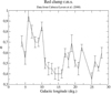 |
Fig. 10 Dispersion of magnitudes in the peak of red clump giants derived by Cabrera-Lavers et al. (2008). |
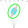 |
Fig. 11 Graphical representation of the model explaining the in-plane observations discussed in this paper. Cyan shows the triaxial bulge; red shows the long bar; green stands for the 3 kpc arm. We set α = 27◦ for the three structures. |
6 Discussion and conclusions
Figure 11 gives a map of the structure in the inner in-plane Galaxy that summarises our achievements from the previous sections: a model with a triaxial bulge plus a long bar and an ellipsoidal ring (3 kpc arm), all of them with angles between the major axis and the line’s Sun–Galactic centre of α = 27◦. Figure 12 represents the amended representation of the whole Galaxy corresponding to the artistic representation of the annotated ‘Road Map to the Milky Way’ by NASA/JPL-Caltech/R. Hurt (SSC/Caltech)3 based on NASA’s Spitzer (Space Infrared Telescope Facility) Space Telescope achievements.
From our analysis, we cannot tell anything about the formation histories of the long bar or the bulge, including whether they are parts of the same structure formed at a given epoch or two different structures formed at two different epochs. Nonetheless, as mentioned in Sect. 1, the evidence presented in the literature supports the hypothesis that the bulge and the long bar are distinct structures; the long bar has stars with different metallicities of the bulge, be they disc-like or higher (González-Fernández et al. 2008; Wegg et al. 2019), and younger ones than those of the bulge at a larger distance from the plane (Ng et al. 1996; Cole & Weinberg 2002). A recent analysis by Nie et al. (2026) reveals a systematic age gradient, with a latitude across the Galactic bulge within 2◦ < |b| < 8◦ shifting from a younger population with an average of  Gyr prevalent near the plane to a predominantly older population with an average of
  Gyr at higher latitudes. A young stellar population at low latitudes is predominantly composed of pseudo-bulges formed via disc/bar processes (incorporating contributions from recent star-forming activity in the Galactic centre; Nataf 2017; Han et al. 2025), whereas the older stellar population is associated with spheroidal bulges generated through early-stage collapse (Obreja et al. 2013) or accretion of debris from merged dwarf galaxies (Obreja et al. 2013). Understanding the long bar as a wing-like extension of the bulge (a thicker structure) is possible too, but with a different period of formation. Calling these younger stars a ‘long bar’ or a ‘peculiar extension of the bulge’ is just a matter of semantics.
With this model, we can explain all of the previous observations. Said explanations are listed below.
Star counts of in-plane bright sources with WISE-4.6µm magnitudes lower than 8 in −10◦ ≲ ℓ ≲ 24◦, either with extinction correction (Fig. 3) or without it (Fig. 1), present a clear asymmetry between positive and negative longitudes. This is explained as the projection of the long bar with the closer part in the first quadrant (López-Corredoira et al. 2007). An angle as in Fig. 11, α ≈ 27◦, is compatible with the estimated angle taking into account the possible tips of the bar,
 deg, from Eq. (4). In particular, using Eq. (3), we can obtain a value of α = 27◦ if we place the tips at ℓ ≈ −9◦, and ℓ = 24◦. With these angles, the semi-axis radius of the long-bar is L0 = 4.3 kpc. One or two degrees of broadening in the tips may be observed due to the thickness of the structure.
For the long bar within 10◦ < ℓ < 24◦, the value of α of the weighted average of the results of the different observations with distance information analysed in this paper is (27.4±1.5) deg; the average of APOGEE M giants with Stone-Martínez et al. (2024) distances is (25.5±2.3) deg (Sect. 3.3); the average of O-rich ones with ages of <5 Gyr (Sect. 4.3) is (28.8±2.0) deg.
The distance distribution of near-plane APOGEE M giants (Fig. 5) or red clumps (K giants) in the literature (see Sect. 5) would observe the long bar too, with a similar angle to Fig. 11. Previous determinations of larger values of the angle α are due to miscalibration of standard candles or the determination of the peak of red clumps in the star counts versus magnitude instead of the density versus distance. The higher spread of distances at 20◦ ≲ ℓ ≲ 30◦ (Fig. 10) would be at the intersection of the long bar with tangential cut of the stellar ring, with an increasing average distance for 24◦ ≲ ℓ ≲ 28◦.
In-plane Miras variable stars with ages of ≲5 Gyr (Figs. 8 and 9) show a remarkable similarity with the proposed scenario. We see the presence of the triaxial bulge within |ℓ| ≲ 10◦ and its extension of the long bar until ℓ = +24◦. We also very clearly see the imprint of the tangential cut of the stellar ring at ℓ ≈ −22◦, which is separated from the bar at negative longitudes and the equivalent point at positive longitudes at ℓ ≈ 27◦; it is at a shorter distance from the tip of the bar, in agreement with previous works (Mikami et al. 1982; Ruelas-Mayorga 1991). Therefore, with this scenario, the tip of the bar in positive longitude would not be at ℓ = −27◦ as previously posited (López-Corredoira et al. 1999, 2007), but at ℓ ≈ 24◦. The proximity of the tip of the bar to the tangential cut of the ring gives place to an almost continuity of stars without any (or with a very small) gap between them. Moreover, the bottom of Fig. 8 shows an almost continuous structure at a heliocentric distance of 4.0−6.0 kpc within −15◦ ≲ ℓ ≲ 30◦, corresponding to the closest part of the near 3 kpc arm, whereas at −25◦ ≲ ℓ ≲ −15◦ we see a much higher spread of heliocentric distances with 5–12 kpc. There is a possible continuation towards the far 3 kpc arm that is tentatively detected beyond the bulge and long bar at certain distances (light green in the bottom part of Fig. 8 at −22◦ ≲ ℓ ≲ +27◦; distances are 9–12 kpc).
In a model of four spiral arms, the peaks in the star counts of the old population as a function of Galactic longitude are explained as (Vallée 2022, Table 8) ℓ = −22◦ being the start of Perseus Arm; ℓ = −12◦ as the start of Sagittarius Arm; ℓ = 19◦ as the start of Norma Arm; and ℓ = 31◦ as the tangential point of the Scutum Arm. However, this Vallée (2017, 2022) model cannot explain some observed features: the almost constant distance of 5.0–5.5 kpc for O-rich Miras between ℓ = 19◦ and ℓ = 27◦ (Fig. 7) or the continuous M giants’ star counts between ℓ = 19◦ and ℓ = 24◦ (Fig. 3). Moreover, spiral arms usually have very young stellar populations, whereas our observations show a significant presence of an old population, either in terms of red clumps (K giants), M giants, or Miras with ages of ≲5 Gyr. Therefore, rather than spiral arms, the presence of the 3 kpc arm (which, in spite of the name, is not a spiral arm, but something of a different nature and part of older stellar populations) better fits the observations.
We solved several controversies concerning the in-plane central area of the Milky Way: an alignment with α ≈ 27◦ between the bulge and the long bar and the 3 kpc arm’s major axis explains everything without the need to introduce different angles for each structure. We also tentatively detect stars from the far 3 kpc arm, and we consistently clarified the nature of the excess of stars at ℓ = −22◦ and ℓ = +27◦ in terms of the tangential cuts of lines of sight with the ellipsoid of the 3 kpc arm. The long bar has a semi-axis radius of around 4 kpc, which is also the size of the major axis of the 3 kpc arm (minor axis ≈3 kpc).
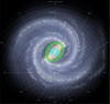 |
Fig. 12 Superposition of model of Fig. 11 with the artistic representation of the annotated ‘Road Map to the Milky Way’ by NASA/JPL-Caltech/R. Hurt (SSC/Caltech) based on NASA’s Spitzer Space Telescope achievements. Note that the angle of the long bar is amended. |
Acknowledgements
Thanks are given to the anonymous referee for helpful comments and suggestions. Thanks are given to the A&A language editor Natasha Saint Geniès. M.L.C. and F.G.L. acknowledge support from the Spanish Min-isterio de Ciencia, Innovación y Universidades (MICINN) under grant number PID2021-129031NB-I00. This publication makes use of data products from the Wide-field Infrared Survey Explorer, which is a joint project of the University of California, Los Angeles, and the Jet Propulsion Laboratory/California Institute of Technology, and NEOWISE, which is a project of the Jet Propulsion Laboratory/California Institute of Technology. WISE and NEOWISE are funded by the National Aeronautics and Space Administration. The AllWISE program is funded by the NASA Science Mission Directorate Astrophysics Division. AllWISE data products are generated using the imaging data collected and processed as part of the original WISE and NEOWISE programs. Funding for the Sloan Digital Sky Survey IV has been provided by the Alfred P. Sloan Foundation, the U.S. Department of Energy Office of Science, and the Participating Institutions. SDSS-IV acknowledges support and resources from the Center for High Performance Computing at the University of Utah. The SDSS website is www.sdss4.org. SDSS-IV is managed by the Astrophysical Research Consortium for the Participating Institutions of the SDSS Collaboration including the Brazilian Participation Group, the Carnegie Institution for Science, Carnegie Mellon University, Center for Astrophysics | Harvard & Smithsonian, the Chilean Participation Group, the French Participation Group, Instituto de Astrofísica de Canarias, The Johns Hopkins University, Kavli Institute for the Physics and Mathematics of the Universe (IPMU) / University of Tokyo, the Korean Participation Group, Lawrence Berkeley National Laboratory, Leibniz Institut für Astrophysik Potsdam (AIP), Max-Planck-Institut für Astronomie (MPIA Heidelberg), Max-Planck-Institut für Astrophysik (MPA Garching), Max-Planck-Institut für Extraterrestrische Physik (MPE), National Astronomical Observatories of China, New Mexico State University, New York University, University of Notre Dame, Observatário Nacional / MCTI, The Ohio State University, Pennsylvania State University, Shanghai Astronomical Observatory, United Kingdom Participation Group, Universidad Nacional Autónoma de México, University of Arizona, University of Colorado Boulder, University of Oxford, University of Portsmouth, University of Utah, University of Virginia, University of Washington, University of Wisconsin, Vanderbilt University, and Yale University. Collaboration Overview Affiliate Institutions Key People in SDSS Collaboration Council Committee on Inclusiveness Architects SDSS-IV Survey Science Teams and Working Groups Code of Conduct SDSS-IV Publication Policy How to Cite SDSS External Collaborator Policy For SDSS-IV Collaboration Members. We acknowledge the use of OGLE survey, a Polish astronomical project based at the University of Warsaw that runs a long-term variability sky survey (1992–present). Most of the observations have been made at the Las Campanas Observatory in Chile. Cooperating institutions include Princeton University and the Carnegie Institution.
References
- Abdurro’uf, Accetta, K., Aerts, C., et al. 2022, ApJS 259, 35 [NASA ADS] [CrossRef] [Google Scholar]
- Abramyan, M. G., Sedrakyan, D. M., & Chalabyan, M. A. 1986, Soviet Astron., 30, 643 [Google Scholar]
- Amôres, E. B., López-Corredoira, M., González-Fernández, C., et al. 2013, A&A, 559, A11 [NASA ADS] [CrossRef] [EDP Sciences] [Google Scholar]
- Anders, F., Khalatyan, A., Chiapini, C., et al. 2019, A&A, 628, A94 [NASA ADS] [CrossRef] [EDP Sciences] [Google Scholar]
- Anders, F., Khalatyan, A., Queiroz, A. B. A., et al. 2022, A&A, 658, A91 [NASA ADS] [CrossRef] [EDP Sciences] [Google Scholar]
- Athanassoula, E. 2005, MNRAS, 358, 1477 [NASA ADS] [CrossRef] [Google Scholar]
- Babusiaux, C., & Gilmore, G. 2005, MNRAS, 358, 1309 [NASA ADS] [CrossRef] [Google Scholar]
- Benjamin, R. A., Churchwell, E., Babler, B. L., et al. 2005, ApJ, 630, L149 [NASA ADS] [CrossRef] [Google Scholar]
- Bettoni, D., & Galleta, G., 1994, A&A 281, 1 [Google Scholar]
- Bilir, S., Ak, T., Ak, S., Yontan, T., & Bostancı, Z. F. 2013, New Astron., 23, 88 [Google Scholar]
- Bland-Hawthorn, J., & Gerhard, O. 2016, Ann. Rev. Astron. Astrophys., 54, 529 [Google Scholar]
- Cabrera-Lavers, A., Hammersley, P. L., González-Fernández, C., et al. 2007, A&A, 465, 825 [NASA ADS] [CrossRef] [EDP Sciences] [Google Scholar]
- Cabrera-Lavers, A., González-Fernández, C., Garzón, F., Hammersley, P. L., & López-Corredoira, M. 2008, A&A, 491, 781 [NASA ADS] [CrossRef] [EDP Sciences] [Google Scholar]
- Catchpole, R. M., Whitelock, P. A., Feast, M. W., et al. 2016, MNRAS, 445, 2216 [Google Scholar]
- Chen, Y. Q., Casagrande, L., Zhao, G., et al. 2017, ApJ, 840, 77 [Google Scholar]
- Chen, B.-H., Kataria, S. K., Shen, J., & Guo, M. 2025, ApJ, 994, 124 [Google Scholar]
- Churchwell, E., Babler, B. L., Meade, M. R., et al. 2009, PASP, 121, 213 [Google Scholar]
- Cole, A. A., & Weinberg, M. D. 2002, ApJ 574, L43 [NASA ADS] [CrossRef] [Google Scholar]
- Compére, P., López-Corredoira, M., & Garzón, F. 2014, A&A, 571, A98 [Google Scholar]
- Covey, K. R, Izević, Z., Schlegel, D., et al. 2007, AJ, 134, 2398 [NASA ADS] [CrossRef] [Google Scholar]
- Cutri, R. M., Wright, E. L., Conrow, T., et al. 2014, https://irsa.ipac.caltech.edu/data/WISE/docs/release/AllWISE/expsup/index.html (Last update: 6 January 2014) [Google Scholar]
- Dame, T. M., & Thaddeus, P. 2008, ApJ, 683, L143 [NASA ADS] [CrossRef] [Google Scholar]
- Dame, T. M., Elmegreen, B. G., Cohen, R. S., & Thaddeus, P. 1986, ApJ, 305, 892 [Google Scholar]
- Davies, B., de la Fuente, D., Najarro, F., et al. 2012, MNRAS, 419, 1860 [NASA ADS] [CrossRef] [Google Scholar]
- Duran, S., & Gökçe, E. Y. 2016, in: The Milky Way and Its Environment (Paris, September 19-23, 2016), https://www.iap.fr/vie_scientifique/ateliers/MilkyWay_Workshop/2016/libdoc/Poster_Duran.pdf [Google Scholar]
- Garzón, F., & López-Corredoira, M. 2014, Astron. Nachr., 335, 865 [Google Scholar]
- Girardi, L., & Salaris, M. 2001, MNRAS, 323, 109 [Google Scholar]
- González-Fernández, C., Cabrera-Lavers, A., Hammersley, P. L., & Garzón, F. 2008, A&A, 479, 131 [NASA ADS] [CrossRef] [EDP Sciences] [Google Scholar]
- González-Fernández, C., López-Corredoira, M., Amôres, E. B., et al. 2012, A&A, 546, A107 [NASA ADS] [CrossRef] [EDP Sciences] [Google Scholar]
- Green, J. A., Caswell, J. L., & McClure-Griffiths, N. M. 2011, ApJ, 733, 27 [NASA ADS] [CrossRef] [Google Scholar]
- Hammersley, P. L., Garzón, F., Mahoney, T., & Calbet, X. 1994, MNRAS, 269, 753 [NASA ADS] [CrossRef] [Google Scholar]
- Hammersley, P. L., Garzón, F., Mahoney, T. J., López-Corredoira, M., & Torres, M. A. P. 2000, MNRAS, 317, L45 [NASA ADS] [CrossRef] [Google Scholar]
- Han, X., Wang, H.-F., Carraro, G., et al. 2025, ApJ, 985, 32 [Google Scholar]
- Hunt, J. A. S., & Vasiliev, E. 2025, New Astron. Rev., 100, 101721 [Google Scholar]
- Iwanek, P., Soszyński, I., & Kozlowski, S. 2021, ApJ, 919, 99 [NASA ADS] [CrossRef] [Google Scholar]
- Iwanek, P., Soszyński, I., Kozlowski, S., et al. 2022, ApJS, 260, 46 [NASA ADS] [CrossRef] [Google Scholar]
- Iwanek, P., Poleski, R., Kozlowski, S., et al. 2023, ApJ, 264, 20 [Google Scholar]
- Karim, T., & Mamajek, E. E. 2017, MNRAS, 465, 472 [NASA ADS] [CrossRef] [Google Scholar]
- Kuijken, K. 1996, IAU Colloq., 169, 71 [Google Scholar]
- Kumar, J., Reid, M. J., & Dame, T. M. 2025, ApJ, 982, 185 [Google Scholar]
- Li, Z.-Y., & Shen, J. 2015, ApJ, 815, L20 [Google Scholar]
- Lockman, F. J. 1980, ApJ, 241, 200 [Google Scholar]
- López-Corredoira, M., Garzón, F., Beckman, J. E., et al. 1999, AJ, 118, 381 [Google Scholar]
- López-Corredoira, M, Hammersley, P. L, Garzón, F., et al. 2001, A&A, 373, 139 [NASA ADS] [CrossRef] [EDP Sciences] [Google Scholar]
- López-Corredoira, M., Cabrera-Lavers, A., Mahoney, T. J., et al. 2007, AJ, 133, 154 [NASA ADS] [CrossRef] [Google Scholar]
- López-Corredoira, M., Cabrera-Lavers, A., González-Fernández, C., et al. 2011, arXiv e-prints [arXiv:1106.0260] [Google Scholar]
- Louis, P. D., & Gerhard, O. E. 1988, MNRAS, 233, 337 [Google Scholar]
- Lucey, M., Pearson, S., Hunt, J. A. S., et al. 2023, MNRAS, 570, 4779 [Google Scholar]
- Mainzer, A., Bauer, J., Grav, T., et al. 2011, ApJ, 731, 53 [Google Scholar]
- Majewski, S. R., Schiavon, R. P., Frinchaboy, P. M., et al. 2017, AJ, 154, 94 [NASA ADS] [CrossRef] [Google Scholar]
- Martínez-Valpuesta, I., & Gerhard, O. 2011, ApJ, 734, L20 [NASA ADS] [CrossRef] [Google Scholar]
- Mikami, T., Ishida, K., Hamajima, K., & Kawara K. 1982, PASJ, 34, 223 [Google Scholar]
- Nataf, D. M. 2017, PASA, 34, e041 [NASA ADS] [CrossRef] [Google Scholar]
- Negueruela, I., González-Fernández, C., Marco, A., Clark, J. S., & Martínez-Núñez, S. 2010, A&A, 513, A74 [NASA ADS] [CrossRef] [EDP Sciences] [Google Scholar]
- Ng, Y. K., Bertelli, G., Chiosi, C., & Bressan, A. 1996, A&A, 310, 771 [NASA ADS] [Google Scholar]
- Nie, J., López-Corredoira, M., Liu, C., Wang, H.-F., & Simion, I. 2026, Res. Astron. Astrophys., 26, 065004 [Google Scholar]
- Obreja, A., Domínguez-Tenreiro, R., Brook, C., et al. 2013, ApJ, 763, 26 [Google Scholar]
- Onozato, H., Ita, Y., & Nakada, Y. 2025, MNRAS, 544, 9110 [Google Scholar]
- Plevne, O., Önal Ta¸s, Ö., Bilir, S., & Seabroke, G. M. 2020, ApJ, 893, 108 [NASA ADS] [CrossRef] [Google Scholar]
- Queiroz, A. B. A., Chiapini, C., Pérez-Villegas, A., et al. 2021, A&A, 656, A156 [NASA ADS] [CrossRef] [EDP Sciences] [Google Scholar]
- Queiroz, A. B. A., Anders, F., Chiappini, C., et al. 2023, A&A, 673, 155 [Google Scholar]
- Ruelas-Mayorga, R. A. 1991, Rev. Mex. Astron. Astrof., 22, 27 [Google Scholar]
- Salaris, M., & Girardi, L. 2002, MNRAS, 337, 332 [NASA ADS] [CrossRef] [Google Scholar]
- Schlegel, D. J., Finkbeiner, D. P., & Davis, M. 1998, ApJ, 500, 525 [Google Scholar]
- Sellwood, J. A., & Wilkinson, A. 1993, Rep. Prog. Phys., 56, 173 [NASA ADS] [CrossRef] [Google Scholar]
- Shen, J., & Debattista, V. P. 2009, ApJ, 690, 758 [Google Scholar]
- Shen, J., & Zheng, X.-W. 2020, RAA, 20, 159 [Google Scholar]
- Stone-Martínez, A., Holtzman, J. A., Imig, J., et al. 2024, AJ, 167, 73 [NASA ADS] [CrossRef] [Google Scholar]
- Vallée, J. P. 2017, Astron. Rev., 13, 1 [Google Scholar]
- Vallée, J. P. 2022, New Astron., 97, 101896 [CrossRef] [Google Scholar]
- van Loon, J., Gilmore, G. F., Omont, A., et al. 2003, MNRAS, 338, 857 [NASA ADS] [CrossRef] [Google Scholar]
- van Woerden, H., Rougoor, G. W., & Oort, J. H. 1957, Comptes Rendus l’Academie des Sciences, 244, 1691 [Google Scholar]
- Wang, S., & Chen, X. 2019, ApJ, 877, 116 [Google Scholar]
- Wegg, C., Gerhard, O., & Portail, M. 2015, MNRAS, 450, 4050 [NASA ADS] [CrossRef] [Google Scholar]
- Wegg, C., Rojas-Arriagada, A., Schultheis, M., & Gerhard, O. 2019, A&A, 632, A121 [NASA ADS] [CrossRef] [EDP Sciences] [Google Scholar]
- Wright, E. L., Eisenhardt, P. R. M., Mainzer, A. K., et al. 2010, AJ, 140, 1868 [Google Scholar]
- Wylie, S. M., Clarke, J. P., & Gerhard, O. E. 2022, A&A, 659, A80 [NASA ADS] [CrossRef] [EDP Sciences] [Google Scholar]
- Yu, Z., Chen, B., Lian, J., Wang, C., & Liu, X. 2025, AJ, 169, 61 [Google Scholar]
- Zasowski, G., 2012, Infrared Extinction and Stellar Structures in the Milky Way Midplane, PhD thesis, University Virginia, USA [Google Scholar]
- Zasowski, G., Benjamin, R. A., & Majewski, S. R. 2012, EPJ Web Conf., 19, 06006 [Google Scholar]
- Zasowski, G., Cohen, R. E., Chojnowski, S. D., et al. 2017, AJ, 154, 198 [Google Scholar]
- Zhang, B., Moscadelli, L., Sato, M., et al. 2014, ApJ, 781, 89 [Google Scholar]
There is an error in López-Corredoira et al. (2007, Eq. (B5)); it should be  instead of
  . In any case, this does not change the estimation of ∆rm when σ << 1.
Appendix A Fit of ellipse parameters
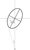 |
Fig. A.1 Graphical representation of an ellipse with a tangential point of a line of sight from the Sun. |
An ellipse has three free parameters: the major axis a, the minor axis b and the angle of the major axis α. It follows
 (A.1)
(A.1)
where (xe,i, ye,i) are coordinates of a point i of the ellipse in the reference system of the ellipse (xe: major axis; ye: minor axis). For each tangential point i = 1, 2 corresponding to lines of sight with Galactic longitude ℓi (see Fig. A.1), we have the direction tangential to the ellipse with angle  (in the system of the ellipse), parallel to the line of sight with Galactic longitude ℓi (in Galactocentric coordinates, with X-axis crossing the Sun), and thus
 (A.2)
(A.2)
Also, this tangential point follows the sine rule
 (A.3)
(A.3)
Another information is the distance d3 of the ellipse at ℓ3 = 0, α3 = −α thus we have a third point i = 3 with
 (A.4)
(A.4)
Therefore, we have five equations (for re,i, i = 1, 2, 3; αi, i = 1, 2) that allow five independent parameters to be determined – three parameters of the ellipse (α, a, b) and the two angles of the tangential points αi, i = 1, 2 – from the five observed numbers ℓi, i = 1, 2, 3; R⊙, d3. The angle α3 is not independent, but equal to α; the values of the radii ri are not independent, but related to αi through Eqs. (A.1).
All Figures
|
Fig. 1 WISE star counts. Top: as a function of ℓ, b within |ℓ| < 40◦, |b| < 5◦, m4.6µm < 8.0, ∆ℓ = 1◦, ∆b = 0.1◦. Bottom: as a function of ℓ within |ℓ| < 40◦, |b| < 0.5◦, for m3.4µm < 8.2, m4.6µm < 8.0, m12µm < 7.0, m22µm < 4.5, ∆ℓ = 1◦. |
| In the text | |
|
Fig. 2 Colour-magnitude diagram in low extincted areas (30◦ < |ℓ| < 40◦, 4◦ < |b| < 5◦; ⟨E(J − K)⟩ = 0.4; Schlegel et al. 1998) for sources with m4.6µm < 8.0. |
| In the text | |
|
Fig. 3 WISE star counts as in Fig. 1 (top panel) but with stars with J − K < 1.0 removed (dwarfs and red clumps from Galactic disc) and with the correction of extinction through Eq. (1). We observe a prominent asymmetry between positive and negative Galactic longitudes and a very slight asymmetry between positive and negative Galactic latitudes. |
| In the text | |
|
Fig. 4 Extinction A4.6µm as a function of ℓ, b within |ℓ| < 40◦, |b| < 5◦; ∆ℓ = 1◦, ∆b = 0.1◦, derived from Eq. (1). |
| In the text | |
|
Fig. 5 Top: APOGEE-2/DR17 M5-6III (−6.5 < MH < −5.5, 1.0 < (J − K)0 < 1.5) star counts, in the range of Galactic coordinates |ℓ| < 40◦, |b| < 5◦. These counts are highly in incomplete (and white areas are unobserved regions) due to the observing strategy of APOGEE-2, but for each line of sight the completeness is constant, with a magnitude within 7.0 < H < 12.2 when AH < 2.7. Bottom: distribution of distances of these stars for −6◦ < ℓ < 30◦, 1.0◦ < |b| < 2.5◦; dashed line shows the best fit to a long bar with an angle of α = 25.6◦ for ℓ > 10◦. |
| In the text | |
|
Fig. 6 Comparison of distances estimated for APOGEE-DR17 with the algorithms of Queiroz et al. (2023) and Stone-Martínez et al. (2024), respectively. |
| In the text | |
|
Fig. 7 Top: O-rich Mira variable star counts, with a period, P, within log10[P(days)] > 2.6, in the range of the Galactic coordinates |ℓ| < 40◦, |b| < 5◦. Bottom: same as the top panel but with the stars within the mask corresponding to regions of high extinction and low completeness removed (see Iwanek et al. 2023). |
| In the text | |
|
Fig. 8 Distribution of distances of O-rich Mira variable stars with a period, P, within log10[P(days)] > 2.6 for −20◦ < ℓ < 30◦, 1.5◦ < |b| < 2.5◦ (top panel; moderate extinction, high completeness) or |b| < 1.5◦ (bottom panel; high extinction, low completeness). The dashed line shows the best fit to a long bar within 10◦ < ℓ < 30◦ for bins with a mask (removing the high-extinction areas), d < R⊙, whereas the dotted line shows the corresponding d(ℓ) for an angle of α = 20.2◦, as fitted for the major axis of the bulge (Iwanek et al. 2023). The dashed cyan line marks a tentative imprint of the far 3 kpc arm. |
| In the text | |
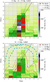 |
Fig. 9 Same stars as Fig. 8 with Cartesian coordinates. |
| In the text | |
|
Fig. 10 Dispersion of magnitudes in the peak of red clump giants derived by Cabrera-Lavers et al. (2008). |
| In the text | |
|
Fig. 11 Graphical representation of the model explaining the in-plane observations discussed in this paper. Cyan shows the triaxial bulge; red shows the long bar; green stands for the 3 kpc arm. We set α = 27◦ for the three structures. |
| In the text | |
|
Fig. 12 Superposition of model of Fig. 11 with the artistic representation of the annotated ‘Road Map to the Milky Way’ by NASA/JPL-Caltech/R. Hurt (SSC/Caltech) based on NASA’s Spitzer Space Telescope achievements. Note that the angle of the long bar is amended. |
| In the text | |
|
Fig. A.1 Graphical representation of an ellipse with a tangential point of a line of sight from the Sun. |
| In the text | |
Current usage metrics show cumulative count of Article Views (full-text article views including HTML views, PDF and ePub downloads, according to the available data) and Abstracts Views on Vision4Press platform.
Data correspond to usage on the plateform after 2015. The current usage metrics is available 48-96 hours after online publication and is updated daily on week days.
Initial download of the metrics may take a while.