| Issue |
A&A
Volume 708, April 2026
|
|
|---|---|---|
| Article Number | A165 | |
| Number of page(s) | 9 | |
| Section | Astrophysical processes | |
| DOI | https://doi.org/10.1051/0004-6361/202558806 | |
| Published online | 03 April 2026 | |
Small-scale turbulent dynamo for low-Prandtl number fluid: Comparison of the theory with results of numerical simulations
1
P. N.Lebedev Physical Institute of RAS, 119991, Leninskij pr.53 Moscow, Russia
2
National Research University Higher School of Economics, 101000, Myasnitskaya 20, Moscow, Russia
★ Corresponding author: This email address is being protected from spambots. You need JavaScript enabled to view it.
Received:
29
December
2025
Accepted:
23
February
2026
Abstract
Context. During the past decades, significant progress has been made in numerical simulations of the turbulent dynamo and the theoretical understanding of turbulence. However, a quantitative comparison between simulations and the theory of the dynamo is still lacking.
Aims. We investigate the generation of a magnetic field by the incompressible turbulent conductive fluid near the critical regime and compare the theoretical predictions of the Kazantsev model with results of recent direct numerical simulations.
Methods. The Kazantsev equation was analyzed both analytically and numerically.
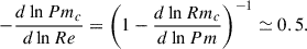
Results. We studied the critical magnetic Reynolds number (Rmc) and the growth rate near the threshold in the limit of very high and for moderate Reynolds numbers. We argue that in the Kazantsev equation for magnetic field generation, the quasi-Lagrangian correlator of velocities should be used instead of the Eulerian, as is usually implied when theory and simulations are compared. The theoretical results obtained with this correlator agree well with the numerical results. We also propose that the decrease of Rmc can be explained as a function of the Reynolds number (Re) at intermediate to high Re. It is probably due to the Reynolds-dependent intermittency of the velocity structure function. We show that the scaling exponent of this function in the inertial range strongly affects the magnetic field generation, and it is known to be an increasing function of the Reynolds number.
Conclusions. The quasi-Lagrangian correlator in the Kazantsev theory provides results that agree well with numerical simulations. An ideal way to compare them is to find the correlator that can be substituted in the Kazantsev equation and the generation properties in the same simulation. Universal parameters at least have to be used, regardless of the properties of the pumping scale. The Reynolds-dependent intermittency can explain the recently observed decrease in the critical magnetic Reynolds number at small Prandtl numbers.
Key words: dynamo / magnetohydrodynamics (MHD) / turbulence / Sun: magnetic fields
© The Authors 2026
 Open Access article, published by EDP Sciences, under the terms of the Creative Commons Attribution License (https://creativecommons.org/licenses/by/4.0), which permits unrestricted use, distribution, and reproduction in any medium, provided the original work is properly cited.
This article is published in open access under the Subscribe to Open model. This email address is being protected from spambots. You need JavaScript enabled to view it. to support open access publication.
1. Introduction
The theory of how magnetic fields appear in turbulent flows of conductive fluid has wide applications, particularly in explaining the magnetic fields observed in many astrophysical objects (see, e.g., Brandenburg & Subramanian 2005; Jouve et al. 2008; Moss et al. 2013; Brandenburg et al. 2024). There are two possible mechanisms to generate a small-scale magnetic field, that is, a field with a characteristic scale much smaller than the integral scale of turbulence (Karak & Brandenburg 2016). First, there is a cascade mechanism of generation that is initiated at large scales under the influence of global shear and convective flows. Second, there is a faster generation process caused by small-scale turbulence. The latter has been studied in numerous papers (see, e.g., Zeldovich et al. 1990; Falkovich et al. 2001; Brandenburg et al. 2012) and is the subject of this paper.
Conductive fluids can be classified by their magnetic Prandtl number,
 (1)
(1)
where ν is viscosity, and η is magnetic diffusivity. For Pm ≫ 1, the resistive scale lies deep inside the viscous range of turbulence (Batchelor 1950; Zel’dovich et al. 1984; Chertkov et al. 1999). This limit is realized, for instance, in the interstellar medium and in processes of star formation (Han 2017). We concentrate on the other case of fluids with low and intermediate Pm. This means that the resistive scale exceeds the viscous scale, so that the excitation of magnetic fluctuations is driven by the inertial-range or bottleneck velocity fluctuations. Low-Pm processes take place in the interior of solar-type stars and planetary convective envelopes (Petrovay & Szakaly 1993).
The theoretical description of the process in the incompressible fluid is based on the Kazantsev equation, which relates the evolution of the magnetic field pair correlator and the velocity structure function. Experimental possibilities are rather limited in terrestrial conditions. Direct numerical simulations (DNS) of low Pm, unlike the case of high Prandtl numbers, face difficulties in modeling magnetic field advection in the inertial range of turbulence and demonstrate some discrepancies between different simulations (see, e.g., Warnecke et al. 2023, Fig. 2).
However, during the past decades, significant progress has been made in the theoretical understanding of the properties of turbulence (L’vov et al. 1997; Donzis & Sreenivasan 2010; Biferale et al. 2011; Iyer et al. 2020) and of the environment and technics of DNS (Iskakov et al. 2007; Warnecke et al. 2023; Rempel et al. 2023; Brandenburg et al. 2023; Yeung et al. 2025), which has resulted in high resolution and advanced to lower values of Pm. This progress gives us hope that we can proceed from a qualitative correspondence to a more or less thorough quantitative comparison at least between theory and DNS.
In the study of turbulence, after the theoretical model formulation (for decaying turbulence) in the classical work (Kolmogorov 1941) and its development for stationary turbulence (Novikov 1965), the precision testing of the model results was performed in experiments (Moisy et al. 1999). The coincidence of theoretical predictions and experimental measurements has, citing Moisy et al. (1999), demonstrated ‘the relevance of isotropic homogeneous turbulence state approximation, used in almost all theoretical approaches to turbulence’. For a low-Pm dynamo, such a program seems hardly possible because of experimental difficulties. However, in the absence of experimental approbation, an accurate quantitative comparison with DNS becomes even more important. It could validate both of the approaches: it would verify the resolution of DNS, and verify the applicability of theoretical assumptions of δ–time correlation (Tobias et al. 2012) and Gaussianity of the turbulent velocity field. It could also test nontrivial effects resulting from non-Gaussianity, for instance, from the weakening of the magnetic field generation, and corrections for the magnetic energy spectrum (Kopyev et al. 2022a,b, 2024). Finally, if the theory were confirmed for moderate to low magnetic Prandtl numbers, it might be scaled to extremely low Pm, which are unattainable by current facilities and typical for astrophysical objects.
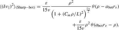
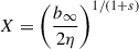
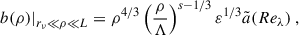
The correct interpretation of numerical data for velocity correlators for their comparison with the theory is one of the problems in this path. In the Kazantsev theory, velocity correlators are assumed to be δ-correlated in time, and the velocity distribution acts in the Kazantsev equation by means of the multiplier b(ρ) in the structure function,
 (2)
(2)
where the longitudinal velocity increments in two near points are
 (3)
(3)
The correlator is independent of t, r, and of the direction of ρ because turbulence is homogeneous and isotropic.
To restore the amplitude b(ρ) from a given correlator, we can use the expression (Vainshtein 1980; Kichatinov 1985)
 (4)
(4)
For the δ -correlated process, there is no difference whether δv∥ is calculated at a fixed point r of space or at an arbitrarily moving point r(t); the correlator is the same. The same result is also obtained for the quasi-Lagrangian reference frame, that is, r(t) tracing one arbitrary fluid particle (L’vov et al. 1997). This frame is distinguished, for example, by the fact that the Kazantsev predictions must be consistent with the results obtained from the evolutionary approach (Zel’dovich et al. 1984; Chertkov et al. 1999) wherever both of the models are applicable; and the evolutionary approach explicitly considers the quasi-Lagrangian frame.
In real turbulent flows, including those in DNS, all structure functions have a nonzero correlation time, and the values of b(ρ) calculated in different frames (i.e., for different r(t) in Eq. (3)) differ essentially. The analysis of data from John Hopkins database shows that at high Reynolds numbers, for all scales ⟨δv∥(ρ, τ)δv∥(ρ, 0)⟩Eul ∝ 1/τ (Kopyev et al., in prep.). If this is so, the logarithmic divergence of Eq. (4) corresponds to a growth of the magnetic field that is faster than exponential; this would contradict the Oseledets theorem (Oseledec 1968). We note that, unlike in the Eulerian case, the quasi-Lagrangian b(ρ) converges well: ⟨δv∥(ρ, τ)δv∥(ρ, 0)⟩Lagr decays exponentially with respect to τ (Biferale et al. 2011).
Consider now some experiment or simulation. We determine below which b(ρ) should be substituted in the Kazantsev equation in order to compare the theory results with the experiment. In other words, we determine which b(ρ) simulates the correct amplitude for the effective δ-correlator. The choice of the Eulerian frame (r = const) in Eq. (3), although it might seem most natural, is in fact not preferable and is probably just incorrect. This might have been the reason that prevented Mason et al. (2011) from obtaining a good correspondence between theory and DNS. A consistent solution of the problem must be based on an accurate dynamical analysis and is far from being performed yet. We assume, however, that the correct answer is to choose the quasi-Lagrangian frame. The grounds for this assumption are as follows:
– First, from the renewing model (Zel’dovich et al. 1984), it follows (Zeldovich et al. 1990; Rogachevskii & Kleeorin 1997) that if the correlation time is shorter than all other characteristic timescales, the quasi-Lagrangian frame gives the correct result: the Kazantsev approach in this case can be verified by evolutionary models. This is even the case near the generation threshold: the characteristic time for the magnetic field evolution is long, so the δ approximation for velocity correlations works well.
– Second, for an arbitrary correlation time but only for high magnetic Prandtl numbers (which restricts the consideration to the viscous range of scales), the choice of the quasi-Lagrangian frame is also correct (Vainshtein 1980; Kichatinov 1985). Recently, Il’yn et al. (2022) have shown the quasi-Lagrangian correlators to be equivalent to effective δ-correlators in long-time approximation.
By analogy with the limit cases, it is reasonable to imply the quasi-Lagrangian velocity increments in Eqs. (3) and (4). The relevance of this assumption is validated in this paper by means of a direct comparison of the predictions of the theory based on the Kaznatsev equation with the velocity structure function b(ρ) determined in this way with the results of DNS. The good agreement is the proof of our choice of the quasi-Lagrangian structure function.
We calculate the critical magnetic Reynolds number and the increments of the magnetic field correlator near the critical regime of generation. For this purpose, we solve the Kazantsev equation with quasi-Lagrangian velocity structure function (4). The basic notations and equations are introduced in Sect. 2.
Unfortunately, there are not many data on quasi-Lagrangian velocity structure functions. We therefore considered two different cases: the Taylor Reynolds number Reλ = 140 (Sect. 3), for which DNS data on the magnetic field (Schekochihin et al. 2007) and velocity correlators (Biferale et al. 2011; Donzis & Sreenivasan 2010) are available, and the limit of the infinite Reynolds number (Sect. 4), where the shape of the velocity correlator is chosen based on theoretical reasons. For this case, we use different approximations and consider the effects produced by the declination of the velocity structure function exponent from the Kolmogorov scaling in the inertial range of turbulence (L’vov et al. 1997; Iyer et al. 2020) and the properties of the transition range between the inertial and largest-eddy scales. We compare the results with the numerical data Iskakov et al. (2007), Schekochihin et al. (2007), Brandenburg et al. (2018), Warnecke et al. (2023) and find a quite good correspondence. We also show that the Reynolds-dependent intermittency of velocity structure functions (Iyer et al. 2020) can explain the observed decrease in the critical Reynolds number at small Prandtl numbers (Warnecke et al. 2023). We calculate the magnetic field correlator growth rate in the vicinity of the generation threshold and compare the results with the DNS (Sect. 5).
Finally, we summarize the results of the paper and comment on further prospects and possible improvements in comparison of the Kazantsev theory predictions with experiments and simulations. In particular, we indicate the properties of quasi-Lagrangian turbulence that can be found from DNS together with the magnetic generation properties, to make the comparison with the theory quantitative (not only qualitative) and precise.
2. Basic equations and parameters
The evolution of the magnetic field B(r, t) is governed by the induction equation,
![Mathematical equation: $$ \begin{aligned} \frac{\partial \boldsymbol{B}(\boldsymbol{r},t)}{\partial t} = \nabla \times \bigl [ \boldsymbol{v}(\boldsymbol{r},t) \times \boldsymbol{B}(\boldsymbol{r},t) \bigr ] + \eta \nabla ^2 \boldsymbol{B}(\boldsymbol{r},t). \end{aligned} $$](/articles/aa/full_html/2026/04/aa58806-25/aa58806-25-eq5.gif) (5)
(5)
Since the back-reaction of the magnetic field on the flow is quadratic in field strength and the initial (seed) magnetic field is weak, we can neglect its effect on the velocity dynamics. In this kinematic regime, the magnetic field acts as a passive vector field advected by the flow. The solenoidal velocity field v(r, t) is treated as a prescribed stochastic field with stationary statistics.
The correlation function of the magnetic field
 (6)
(6)
is assumed to be independent of r in a homogenous isotropic flow. Its evolution under the assumption (2) is described by the equation (Kazantsev 1968)
 (7)
(7)
where
and the function b(ρ) is defined in (4). We are interested in the exponential behavior of the magnetic field, and we therefore searched for a solution in the form
Then, ψ satisfies the Schrodinger-type equation (Kazantsev 1968)
 (8)
(8)
 (9)
(9)
 (10)
(10)
with the boundary condition ψ(0) = 0, ψ(∞) < ∞. We solved this equation numerically by means of a modification of the stochastic quantization idea (Il’yn et al. 2021, Appendix A).
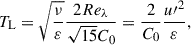
To compare the theory with the results of DNS, we normalized the dimensional parameters. Generally, an isotropic hydrodynamical flow is completely characterized by three dimensional parameters (Novikov 1965; Moisy et al. 1999):
where ν is the viscosity, ε is the total energy flux from larger to smaller scales, and vrms is the volume integrated root-mean-squared velocity. From these three parameters, we composed one universal dimensionless combination, for example,
 (11)
(11)
where  is the Taylor scale; this parameter is called the Taylor Reynolds number. However, the classical Reynolds number is often used,

where L is the pumping scale, or the largest-eddies scale, and is not defined universally. This uncertainty produces difficulties in matching different experimental and/or DNS results and their comparison with the theory (e.g., Brandenburg et al. 2018 reported some obstacles when comparing their results with those of Schekochihin et al. 2007). We defined
 (12)
(12)
This corresponds to the relations between Re and Reλ used by Schekochihin et al. (2007).
The magnetic properties of the fluid can be described by the dimensionless magnetic Prandtl number (1). The magnetic Reynolds number
 (13)
(13)
is also generally used. Unlike Pm, it depends on the choice of L in the definition of the Reynolds number.
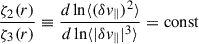
We are interested in the stability condition Pmc(Reλ), or Rmc(Re) such that there is a solution of (8) with γ = 0 and there is no solution with γ > 0 for smaller Rm. We note that the second relation is conventional, but the first one is more universally defined.
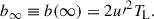
In the vicinity of this stability curve, γ is known to depend log-linearly on Rm (Rogachevskii & Kleeorin 1997; Kleeorin & Rogachevskii 2012),

Based on Eq. (8), we calculated the proportionality coefficient numerically and compared it with the results of Warnecke et al. (2023). To solve Eq. (8), we assumed some model for b(ρ). This produced one more difficulty, since b(ρ) is the quasi-Lagrangian correlation function and is difficult to measure (Biferale et al. 2011). By definition of the Lagrangian correlation time τc(ρ) introduced by L’vov et al. (1997), we have
 (14)
(14)
In Biferale et al. (2011), Donzis & Sreenivasan (2010), the simultaneous structure function ⟨(δv∥)2⟩ and the correlation time τc were found from DNS for Reλ = 140; for much higher Reλ, we used theoretical considerations (L’vov et al. 1997) that argue that both ⟨(δv∥)2⟩ and τc are power-law functions of ρ inside the inertial range.
3. Reλ = 140: Moderate Re and Pm
In this section, we refer to the results of Biferale et al. (2011), Donzis & Sreenivasan (2010) for data on velocity statistics and Iskakov et al. (2007), Schekochihin et al. (2007) for data on magnetic generation. Fortunately, all these papers contained the DNS performed for the same Reynolds number Reλ = 140. The critical Prandtl number is not small for this Reynolds number, so the bottleneck region and even the viscous range of scales can affect the results and have to be taken into account. The main parameters of the DNS performed by Biferale et al. (2011) are listed in Table 1.
Main parameters of the flow with Reλ = 140.
Biferale et al. (2011) calculated the dependence of the Lagrangian correlation time τc on ρ,
 (15)
(15)
where

rν = ν3/4ε−1/4 is the Kolmogorov viscous scale, and  is the viscous characteristic time.
The second-order simultaneous velocity structure function is well investigated; in the viscous and inertial ranges, its behavior is universal and is very well described by the generalized Batchelor approximation (Donzis & Sreenivasan 2010),
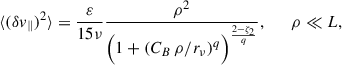 (16)
(16)

It is easy to see that in the ultraviolet regime, it coincides with Kolmogorov’s analytical formula, 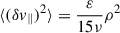 , ρ ≪ rν, while inside the inertial range, it demonstrates a power-law behavior, ⟨(δv∥)2⟩∝ρζ2, L ≫ ρ ≫ rν/CB. We note that the coefficients CB in Eq. (16) and C2 in Eq. (15) are both comparably small. This corresponds to the existence of the bottleneck transition region between the viscous and the inertial ranges: viscosity is essential at scales ρ ∼ rν/C2 ≃ rν/CB, which are significantly larger than the viscous scale.
For our purpose, we enlarged the limits of applicability of Eq. (16) for larger scales up to the integral scale, where ⟨(δv∥)2⟩ = 2u′2, ρ ≥ L. In accordance with the idea of extended self-similarity (ESS), this can also be done by means of a fractionally rational approximation1,
 (17)
(17)
where Cm = 1.6 follows from the matching with the integral scale.
The two transitional regions, the bottleneck and the range between the inertial and integral scales, are presented in Eq. (17) by the two brackets in the denominator. To estimate the accuracy of the approximation and to visualize the contributions of the two transition regions, we consecutively substituted a piecewise power-law function for each of the brackets,
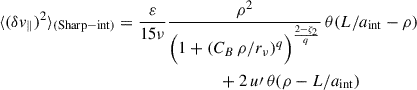 (18)
(18)
and
 (19)
(19)
The coefficients abot = 13.1 and aint = 1.6 were also found from the matching condition, as were CB and Cm. The value of aint coincides to high accuracy with Cm, which indicates that the two approximations are rather close.
The results are presented in Table 2. The theoretical predictions are rather close to the numerical results; the use of the Eulerian structure function b(ρ) would give an estimate of Rmc at least an order of magnitude lower. The fact that the theoretical prediction for Rmc is lower than the experimental result may be caused by the assumption of Gaussianity of the flow: when the declination from Gaussianity is taken into account, that is, the third-order correlator of the velocity, the result can increase (Kopyev et al. 2024).
Results of the Kazantsev equation analysis and DNS (Reλ = 140).
The critical values of the magnetic Reynolds number and Prandtl number are close for all the three models, but the results still differ by about 15%. This indicates the effect of the transitional regions on the near-threshold generation. The importance of the bottleneck region is determined by the fact that the magnetic Prandtl number is not small enough to neglect the effect of the viscous range. From the value of CB in Eq. (17) and C2 in Eq. (15), it follows that the effect of the viscosity reaches about 15rν, while for Pm = 0.25, the magnetic diffusivity scale is only about 3rν, so it lies deep inside the bottleneck range. It is natural to assume that for smaller Pm, the effect of viscosity on the magnetic field generation decreases. In contrast, the effect of the external transition between the inertial and the integral ranges can only become even stronger for higher Reynolds numbers.
4. Very high Reynolds numbers
The lack of experimental or DNS data on the hydrodynamic Lagrangian correlation time prevented us from determining b(ρ) for other Reynolds numbers, and, hence, from calculating Rmc for them. However, for a well-developed turbulence with a wide inertial range, we assumed in accordance with the general theoretical approach to turbulence that b(ρ) has a universal shape regardless of the details of the flow. To normalize the function, we took the largest scales. For these scales,
 (20)
(20)
and the integral Lagrangian correlation time  can be found from the approximation based on Sawford’s second-order stochastic model (Sawford 1991; Sawford et al. 2008),
 (21)
(21)
where C0 is the Kolmogorov constant. It is rather difficult to find (Lien & D’Asaro 2002; Ouellette et al. 2006; Zimmermann et al. 2010; Uma-Vaideswaran & Yeung 2025), and we used the value obtained by Sawford & Yeung (2011),
 (22)
(22)
In what follows, we therefore consider different models for b(ρ) that satisfy the normalization condition consistent with Eq. (14)
 (23)
(23)
According to Eqs. (21), (11),(1),
 (24)
(24)
In what follows, we use the dimensionless value
 (25)
(25)
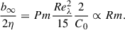
to characterize the generation properties of a flow. Here, s is the scaling exponent of ⟨|δv∥|⟩. The value of X describes the relative width of the range of scales that can affect the generation. We note that for any particular series of DNS or experiments, Rm ∝ X1 + s, but because the definition of the integral scale L is uncertain, X is more accurately defined than Rm.
4.1. Sharp model
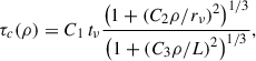
We started with the natural and simple theoretical model proposed by Vainshtein & Kichatinov (1986), which focuses on the main features of turbulence (hereinafter, model ‘Sharp’). It describes the power-law behavior of b(ρ) in the inertial range and its approximate constancy at large scales,
 (26)
(26)
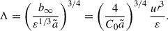
This model was used in numerous papers (see, e.g., Rogachevskii & Kleeorin 1997; Vincenzi 2002; Boldyrev & Cattaneo 2004; Arponen & Horvai 2007; Schober et al. 2012; Kleeorin & Rogachevskii 2012; Kopyev et al. 2026). The viscous range is not of interest for a dynamo study at very high Reynolds numbers, since it is far below the magnetic diffusion scale and cannot contribute to the generation. The integral scale L used in the definition of Re, Rm was assumed to be proportional to Λ. The sharp break in Eq. (26) results in a kink in σ(ρ) and in a discontinuity in σ′. This discontinuity produces a δ-function in the potential (9). This is a peculiar property of the model and just enhances and emphasizes the maximum of U(ρ), but the term ρσ′ does not play an essential role. It changes the resulting Rmc to only about 20% (Kopyev et al. 2026). A much larger contribution to Rmc is produced by the sharp kink at the same ρ = Λ.
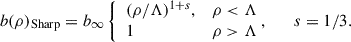
From Eq. (25), X is the ratio of the end of the inertial range scale Λ and the magnetic diffusion scale rd,
Kopyev et al. (2026) reported that the generation threshold corresponds to a critical value of X equal to

Then, according to Eq. (24) and Eq. (12),
In what follows, we compare this result with the results of other models.
4.2. Intermittency: Dependence on s
The scaling exponent of b inside the inertial range is an important parameter. It is composed of the exponents of ⟨(δv∥)2⟩ and τc. Let ⟨|δv∥|n⟩∝ρζn ; then, according to the bridge relations (L’vov et al. 1997; Biferale et al. 2011), τc ∝ ρ1 − ζ2 + ζ1 and, hence,
 (27)
(27)
In the Kolmogorov phenomenological theory, we obtain s = ζ1 = 1/3. However, the intermittency of the velocity structure functions implies that ζn > n/3 for n < 3 (Frisch 1995).
The values of ζn depend on Re; for very high Reynolds numbers (Reλ ≳ 650), we obtain s = ζ1 = 0.39 (Benzi et al. 2010; Iyer et al. 2020). Even this small change in s affects the generation properties significantly: for s = 0.39, we obtain Xc = 14.6, which results in smaller critical Reynolds number,
This qualitative behavior is an important indication for the explaination of the decrease in Rmc for high enough Reynolds numbers. Iyer et al. (2020) showed that ζ1 increases as a function of Re. This is a sufficient reason for the decrease in Rmc observed by Warnecke et al. (2023).
4.3. Smooth model: Effect of the transition region
Not only the inertial range, but also the transition scales from the inertial to the integral range affect the generation of high Reynolds numbers. To demonstrate this, we considered the ’Smooth’ model: it coincides with the Sharp model in the inertial and integral ranges, but provides a more accurate description in between,
 (28)
(28)
Since at ρ ≪ Λ and at ρ → ∞ this coincides with bSharp, the definition of rd and the relation X = Λ/rd remain the same. The shape of b(ρ) for the Smooth and Sharp models is illustrated in Fig. 1.
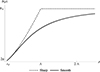 |
Fig. 1. Shape of b(ρ) for the Sharp (Eq. (26)) and Smooth (Eq. (28)) models for the same values of the parameters s, b∞, and Λ. |
We considered the Smooth model with a classical nonintermittent scaling s = 1/3 and with a more realistic s = 0.39. The resulting Xc and RmcSch are presented in Table 3. Comparing the results of the theoretical models with the DNS data, we found that the agreement is quite reasonable. All the models show a value of Rmc lower than the upper limit RmcSch ≤ 350 found by Schekochihin et al. (2007). The data of Schekochihin et al. (2007), Iskakov et al. (2007), Warnecke et al. (2023) demonstrate the decrease in Rmc at Reλ ≳ 300, and the value of Rmc obtained at the highest Reynolds number Re ≃ 5 ⋅ 104 achieved by Warnecke et al. (2023)2 is RmcSch ≳ 200. This agrees very well with the prediction of the Smooth model for s = 0.39, which is the most realistic of our models.
Results for very high Reynolds numbers.
Comparison of the Smooth and Sharp models shows that the effect of the transition region is significant: the critical values of the parameters differ by almost a factor of two. We determine the reason of the difference below.
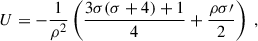
The velocity correlator profiles and the corresponding potentials U(ρ) drawn at the critical values Λc are rather close in both models everywhere except in the vicinity of Λc(Sharp) (see Fig. 2). This appears to be the region in which the transition zone has the strongest effect. On the other hand, this is the boundary of the region in which the generation occurs. The generation threshold at any given Reynolds number corresponds to the zero energy level; Fig 2 shows that the scales ρ0 : U(ρ0) = 0 for the Smooth models differ by less than 20% from the corresponding scales ρ0(Sharp) = Λc(Sharp) for the Sharp models. Hence, the generation region ρ ≲ ρ0 is situated for the Sharp and Smooth models within or near the scale Λc(Sharp) and rather far from the integral scale Λc(Smooth). Although the Sharp model is less plausible and accurate than the Smooth model, it indicates the scales that contribute most to the generation better.
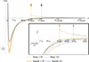 |
Fig. 2. Effective potential U(ρ) (Eq. (9)) that corresponds to the generation threshold for the two Sharp and two Smooth models. The length scale is normalized by the diffusion scale rd, which is taken to be the same for both models. The vertical arrows correspond to the δ functions in the Sharp model potential. |
The difference in the values of Rmc is therefore probably caused by different meanings of the scale Λ in the two types of models. While Λc(Smooth) corresponds to the integral scale of turbulence, Λc(Sharp) merely acts as a transition range marker, which is about twice smaller.
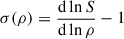
The function b(ρ) contributes to U(ρ) by means of the logarithmic derivative σ(ρ). It is therefore interesting to compare these functions in critical regimes for different models. In Fig. 3 the functions σ(ρ) that correspond to the generation threshold are plotted. The rising parts of the curves are almost identical, the whole difference being in the descending part of the curve. In accordance with Kazantsev (1968), the scales important for the generation satisfy the condition σ > 0. For every s, the graphs for both models intersect the line σ = 0 at ρ ≃ Λc(Sharp). This shows that the Kazantsev criterion agrees well with the criterion ρ ≲ ρ0.
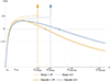 |
Fig. 3. Logarithmic derivative σ(ρ), Eq. (10), for the four models. The length scale is normalized by the same rd. The parameters of each model correspond to the generation threshold. |
The transition region probably determines the generation boundary. On the other hand, in the absence of the self-similarity of velocity correlators at the largest scales, the properties of this transition region may not be uniquely related to the velocity properties at the integral scales. If this is so, the comparison of some characteristics related to the transition region, for example, ρ0 or the scale at which σ = 0 for different DNS-s or experiments, would be more effective than the comparison of large-scale parameters such as the magnetic Reynolds numbers.
In other words, it may be more effective to describe the generation threshold by means of some combination of parameters that describe the surrounding of the point ρ0 or ρ : σ = 0 rather than by means of integral characteristics such as Rmc.
5. Increment near the generation threshold
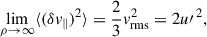
We considered the growth rate 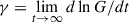 of the magnetic field correlator near the generation threshold. Namely, we were interested in
We note that since the expression contains the ratio Rm/Rmc , it does not depend on the choice of normalization.
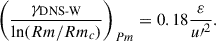
Rogachevskii & Kleeorin (1997), Kleeorin & Rogachevskii (2012) predicted this value to be constant along the critical curve (Rm = Rmc) for small Prandtl numbers. The data of Warnecke et al. (2023) confirmed this prediction for a wide range of Prandtl numbers beginning with Pm ≲ 0.1. The value of the coefficient found by Brandenburg et al. (2018), Warnecke et al. (2023) is
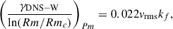
where kf is the pumping wave number; taking the relation ε/(vrms3kf) = 0.041 given by Brandenburg et al. (2018) into account, we can express this in terms of universal variables,
 (29)
(29)
To compare this coefficient with the Kazantsev theory, we were again forced to take the value Reλ = 140, since for this Reynolds number, we have information on the Lagrangian statistics (Biferale et al. 2011). The Prandtl number corresponding to this Reλ is Pm ≈ 0.3 and does not belong to the range in which the increment slope is constant. However, according to the data of Warnecke et al. (2023), the value is close to the boundary and the slope does not differ significantly.
Making use of the velocity statistics given by Biferale et al. (2011), Donzis & Sreenivasan (2010), we solved Eq. (8) numerically for values of γ close to zero and obtained (for Reλ = 140)
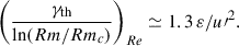 (30)
(30)
To compare this with Eq. (29), we note that the increment derivatives in Eq. (29) are taken at constant Prandtl numbers, while in Eq. (30), they are taken at constant Reynolds numbers. These two derivatives are related by
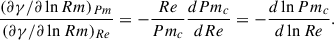
This follows from Eq. (13) and from the condition that γ = 0 along the critical curve Rmc(Re). From the data presented by Schekochihin et al. (2007), Warnecke et al. (2023), we found
The results for the theoretical calculation and for the DNS results are summarized in Table 5. We also added g obtained from the DNS data (Schekochihin et al. 2007) (see Table 4),
 (31)
(31)
Simulation data of Schekochihin et al. (2007)
The results differ significantly. Even the results of the two numerical simulations are quite different; when this is taken into account, the fact that the theoretical and numerical results are on the same order is a good correspondence.
The significant difference between the theoretical and numerical results can be explained as follows, for example:
– The data for hydrodynamics are taken from different sources, and this affects the errors strongly. In particular, C0 is difficult to determine and depends strongly on the isotropy of the flow and other factors. We used the value (22) found analytically (Sawford 1991) in the frame of a particular model. The difference given by various DNSs and experiments is up to 1.5 times in both directions (Lien & D’Asaro 2002; Uma-Vaideswaran & Yeung 2025).
– In Table 4 the estimate of the slope of a curve near the inflection point is taken by only two distant points, which may lead to an underestimation of the slope. In addition, these two points are themselves known to have some errors.
– The details of DNS, such as periodic boundary conditions, can affect the generation.
– Finally, the real slope may be smaller than the one predicted by the Kazantsev model because of the non-Gaussianity of the velocity flow. If this factor were taken into account, the slope would decrease (Kopyev et al. 2024).
In the case of high Reynolds numbers, we lack enough data for nonsimultaneous velocity statistics, and we restricted ourselves by dimensional considerations. For the Sharp and Smooth models, we obtained inside the inertial range of scales
 (32)
(32)
where  is a dimensionless parameter. As Re → ∞, the function
  has a constant limit (Frisch 1995). Taking Eq. (23) into account, we obtain for the Sharp model from the condition b(Λ) = b∞
For the Smooth model, the result differs no more than by a multiplier of ∼2. Then, the increment is
This confirms that the increment does not depend on the Reynolds number for very high Re. Kleeorin & Rogachevskii (2012) obtained this result for s = 1/3; we prove that the presence of intermittency practically does not affect it, so that the independence of g is preserved up to the values of Re at which the bottleneck effect is essential.
6. Discussion
We studied the magnetic field generation in a turbulent flow near the generation threshold. We compared theoretical predictions of the extended Kazantsev theory with results of DNS for two cases: the value of the local Reynolds number Reλ = 140, which is distinguished by the presence of magnetohydrodynamical and Lagrangian hydrodynamical data, and the limiting case of very high Reynolds numbers. To calculate the time-integrated velocity structure function b(ρ) (see Eq. (4)), we used the quasi-Lagrangian statistics (in particular, the Lagrangian velocity correlation time). This provided a better concordance with the DNS results by some orders of magnitude than those found with the Eulerian statistics. The values of critical magnetic Reynolds and magnetic Prandtl numbers obtained from the theory and from DNS differ by no more than ∼10%.
An ideal way to compare the DNS with theory should be to find b(ρ) and Pmc in the same DNS and to solve Eq. (8) with this particular b(ρ). Even when we neglect the term with σ′ (which is difficult to calculate numerically) in the potential, we would obtain a rather high accuracy of presumably better than 20%. In this sense, the Kazantsev equation is a type of bridge connecting quasi-Lagrangian turbulence to the parameters of the magnetic field generation.
In absence of such a combined DNS, we took the data of Biferale et al. (2011), Donzis & Sreenivasan (2010) for the velocity statistics for one particular Reynolds number and compared the result with the data of Schekochihin et al. (2007). The result is presented in Table 2, and the agreement is quite good.
One more difficulty for the comparison of the theory and the numerical/experimental data is the use of different normalizations by different authors. This creates ambiguity and the additional need to coordinate data. In order to avoid this, it would be better to provide the stability curve in terms of Pmc as a function of Reλ, since, unlike Rm and Re, they are independent of the pumping properties of a particular flow and are universal in the sense that they can be expressed in terms of the basic parameters ε, vrms, ν, η. Another way is to use a more universal definition of the integral scale. We presented our results in terms of ReSch, RmSch that are defined by Eqs. (12) and (13).
The comparison of different models shows the importance of the transition region between the inertial and the integral ranges. While the bottleneck transition between the viscous and inertial ranges is only important for relatively small Reynolds numbers, this outer transition range was found to be essential for the magnetic field generation at all Reynolds numbers.
For extremely high Reynolds numbers, the piecewise power-law model (Sharp) represents the qualitative properties of the generation well, but lowers the generation threshold significantly; the Smooth model appears to be much more accurate and agreed well with DNS. For the velocity scaling exponent found by Iyer et al. (2020), the obtained critical magnetic Reynolds number fits the DNS results well.
The comparison of the Sharp and the Smooth models helped us to determine the region that is most important for the value of the generation threshold. It is about twice smaller than the parameter Λ of the Smooth model, which is comparable to the pumping scale. This scale belongs to the transition region from the inertial to the pumping range. It can be marked by the condition σ(ρ)≈dlnb/dlnρ = 0, or by the claim that the effective potential (9) is zero at the point.
Based on the comparison of our data for different scaling exponents, we propose an explanation of the decrease in the critical magnetic Reynolds number as a function of Re for 650 ≳ Reλ ≳ 300. The earlier explanation referred to the effect of the bottleneck, but the downward tendency of Rmc also continues for Pm ≲ 0.01, where the effect of the bottleneck is certainly negligible. We note that the critical magnetic Reynolds number depends essentially on the scaling exponent of the velocity structure function inside the inertial range. As shown by Iyer et al. (2020), the scaling exponent decreases as a function of Re from one-third at relatively small Re to 0.39 as Re → ∞. This decrease is enough to ensure the decrease in Rmc.
We also studied the dependence of the growth rate exponent of the magnetic field correlator on the magnetic Reynolds number. The results are presented in Table 5. The theoretical prediction differs by two to four times from the numerical results, which in turn differ significantly from each other. On one hand, this is a good correspondence taking into account the technical uncertainties. On the other hand, the difference might be decreased when the non-Gaussianity of the velocity field is taken into account. As in the case of Rmc, the corresponding correction would change the theoretical result in the right direction.
Results for the increment slope.
To conclude, we stress the importance of a precise comparison of the kinematic dynamo theory with DNS. It would quantitatively verify the key theoretical simplifications, such as a δ-correlated in time effective velocity field. We obtained encouraging results, which confirm this assumption, by an attempt of such a comparison using the existing numerical and theoretical data on turbulence. We hope that future DNSs will be able to combine kinematic dynamo and Lagrangian velocity properties, which would allow for an accurate comparison with the Kazantsev theory. The precise comparison would also allow for a quantitative assessment of the effect of non-Gaussian effects, such as dynamo suppression and changes in the magnetic energy spectrum. A successful confirmation of the theory at moderately low magnetic Prandtl numbers would provide a critical basis for the extrapolation of its predictions to extreme, astrophysically significant Pm values, which are beyond our current computational capabilities.
Acknowledgments
This work of AVK was supported by the Foundation for the Advancement of Theoretical Physics and Mathematics (BASIS).
References
- Arponen, H., & Horvai, P. 2007, J. Stat. Phys., 129, 205 [Google Scholar]
- Batchelor, G. K. 1950, Proc. Royal Soc. London. Ser. A. Math. Phys. Sci., 201, 405 [Google Scholar]
- Benzi, R., Biferale, L., Fisher, R., Lamb, D. Q., & Toschi, F. 2010, J. Fluid Mech., 653, 221 [NASA ADS] [CrossRef] [Google Scholar]
- Benzi, R., Ciliberto, S., Tripiccione, R., et al. 1993, Phys. Rev. E, 48, R29 [CrossRef] [Google Scholar]
- Biferale, L., Calzavarini, E., & Toschi, F. 2011, Phys. Fluids, 23 [Google Scholar]
- Boldyrev, S., & Cattaneo, F. 2004, Phys. Rev. Lett., 92, 144501 [Google Scholar]
- Brandenburg, A., & Subramanian, K. 2005, Phys. Rep., 417, 1 [NASA ADS] [CrossRef] [Google Scholar]
- Brandenburg, A., Sokoloff, D. D., & Subramanian, K. 2012, Space Sci. Rev., 169, 123 [Google Scholar]
- Brandenburg, A., Haugen, N. E. L., Li, X.-Y., & Subramanian, K. 2018, MNRAS, 479, 2827 [Google Scholar]
- Brandenburg, A., Rogachevskii, I., & Schober, J. 2023, MNRAS, 518, 6367 [Google Scholar]
- Brandenburg, A., Neronov, A., & Vazza, F. 2024, A&A, 687, A186 [NASA ADS] [CrossRef] [EDP Sciences] [Google Scholar]
- Chertkov, M., Falkovich, G., Kolokolov, I., & Vergassola, M. 1999, Phys. Rev. Lett., 83, 4065 [Google Scholar]
- Donzis, D. A., & Sreenivasan, K. R. 2010, J. Fluid Mech., 657, 171 [Google Scholar]
- Falkovich, G., Gawedzki, K., & Vergassola, M. 2001, Rev. Mod. Phys., 73, 913 [Google Scholar]
- Frisch, U. 1995, Turbulence: the Legacy of A.N. Kolmogorov (Cambridge: Cambridge University Press) [Google Scholar]
- Han, J. L. 2017, ARA&A, 55, 111 [NASA ADS] [CrossRef] [Google Scholar]
- Il’yn, A. S., Kopyev, A. V., Sirota, V. A., & Zybin, K. P. 2021, Phys. Fluids, 33 [Google Scholar]
- Il’yn, A. S., Kopyev, A. V., Sirota, V. A., & Zybin, K. P. 2022, Phys. Rev. E, 105, 054130 [Google Scholar]
- Iskakov, A. B., Schekochihin, A. A., Cowley, S. C., McWilliams, J. C., & Proctor, M. R. E. 2007, Phys. Rev. Lett., 98, 208501 [NASA ADS] [CrossRef] [Google Scholar]
- Iyer, K. P., Sreenivasan, K. R., & Yeung, P. K. 2020, Phys. Rev. Fluids, 5, 054605 [Google Scholar]
- Jouve, L., Brun, A. S., Arlt, R., et al. 2008, A&A, 483, 949 [NASA ADS] [CrossRef] [EDP Sciences] [Google Scholar]
- Karak, B. B., & Brandenburg, A. 2016, ApJ, 816, 28 [Google Scholar]
- Kazantsev, A. P. 1968, Sov. Phys. JETP, 26, 1031 [Google Scholar]
- Kichatinov, L. L. 1985, Magnetohydrodynamics, 21, 1 [Google Scholar]
- Kleeorin, N., & Rogachevskii, I. 2012, Phys. Scr., 86, 018404 [Google Scholar]
- Kolmogorov, A. N. 1941, Dokl. Akad. Nauk SSSR, 32, 19 [Google Scholar]
- Kopyev, A. V., Il’yn, A. S., Sirota, V. A., & Zybin, K. P. 2022a, Phys. Fluids, 34 [Google Scholar]
- Kopyev, A. V., Kiselev, A. M., Il’yn, A. S., Sirota, V. A., & Zybin, K. P. 2022b, ApJ, 927, 172 [NASA ADS] [CrossRef] [Google Scholar]
- Kopyev, A. V., Il’yn, A. S., Sirota, V. A., & Zybin, K. P. 2024, MNRAS, 527, 1055 [Google Scholar]
- Kopyev, A. V., Sirota, V. A., Il’yn, A. S., & Zybin, K. P. 2026, Phys. Rev. E, 113, 035101 [Google Scholar]
- Lien, R.-C., & D’Asaro, E. A. 2002, Phys. Fluids, 14, 4456 [Google Scholar]
- L’vov, V. S., Podivilov, E., & Procaccia, I. 1997, Phys. Rev. E, 55, 7030 [Google Scholar]
- Mason, J., Malyshkin, L., Boldyrev, S., & Cattaneo, F. 2011, ApJ, 730, 86 [Google Scholar]
- Moisy, F., Tabeling, P., & Willaime, H. 1999, Phys. Rev. Lett., 82, 3994 [Google Scholar]
- Moss, D., Kitchatinov, L. L., & Sokoloff, D. D. 2013, A&A, 550, L9 [NASA ADS] [CrossRef] [EDP Sciences] [Google Scholar]
- Novikov, E. A. 1965, Sov. Phys. JETP, 20, 1290 [Google Scholar]
- Oseledec, V. I. 1968, Trans. Moscow Math. Soc., 19, 197 [Google Scholar]
- Ouellette, N. T., Xu, H., Bourgoin, M., & Bodenschatz, E. 2006, New J. Phys., 8, 102 [Google Scholar]
- Petrovay, K., & Szakaly, G. 1993, A&A, 274, 543 [Google Scholar]
- Rempel, M., Bhatia, T., Bellot Rubio, L., & Korpi-Lagg, M. J. 2023, Space Sci. Rev., 219, 36 [NASA ADS] [CrossRef] [Google Scholar]
- Rogachevskii, I., & Kleeorin, N. 1997, Phys. Rev. E, 56, 417 [NASA ADS] [CrossRef] [Google Scholar]
- Sawford, B. L. 1991, Phys. Fluids A: Fluid Dyn., 3, 1577 [Google Scholar]
- Sawford, B. L., & Yeung, P.-K. 2011, Phys. Fluids, 23 [Google Scholar]
- Sawford, B. L., Yeung, P.-K., & Hackl, J. F. 2008, Phys. Fluids, 20, 065111 [Google Scholar]
- Schekochihin, A. A., Iskakov, A. B., Cowley, S. C., et al. 2007, New J. Phys., 9, 300 [Google Scholar]
- Schober, J., Schleicher, D., Bovino, S., & Klessen, R. S. 2012, Phys. Rev. E, 86, 066412 [NASA ADS] [CrossRef] [Google Scholar]
- Tobias, S., Cattaneo, F., & Boldyrev, S. 2012, MHD Dynamos and Turbulence in "Ten Chapters in Turbulence" (Cambridge: Cambridge University Press), 351 [Google Scholar]
- Uma-Vaideswaran, R., & Yeung, P. K. 2025, ArXiv e-prints [arXiv:2512.17078] [Google Scholar]
- Vainshtein, S. I. 1980, Sov. Phys. JETP, 52, 1099 [Google Scholar]
- Vainshtein, S. I., & Kichatinov, L. L. 1986, J. Fluid Mech., 168, 73 [Google Scholar]
- Vincenzi, D. 2002, J. Stat. Phys., 106, 1073 [Google Scholar]
- Warnecke, J., Korpi-Lagg, M. J., Gent, F. A., & Rheinhardt, M. 2023, Nat. Astron., 7, 662 [NASA ADS] [CrossRef] [Google Scholar]
- Yeung, P. K., Ravikumar, K., Uma-Vaideswaran, R., et al. 2025, J. Fluid Mech., 1019, R2 [Google Scholar]
- Zel’dovich, Y. B., Ruzmaikin, A. A., Molchanov, S. A., & Sokoloff, D. D. 1984, J. Fluid Mech., 144, 1 [Google Scholar]
- Zeldovich, Y. B., Ruzmaikin, A. A., & Sokoloff, D. D. 1990, The Almighty Chance (World Scientific) [Google Scholar]
- Zimmermann, R., Xu, H., Gasteuil, Y., et al. 2010, Rev. Sci. Instrum., 81 [Google Scholar]
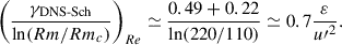
The paper Warnecke et al. (2023) reports Rmc ≈ 102, but the normalization of Re and Rm that is used there is about two times lower than that of Schekochihin et al. (2007), Iskakov et al. (2007): according to Brandenburg et al. (2018), the definition of Re (and, hence, Rm) in Brandenburg et al. (2018) is probably 1.5 times smaller than those in Iskakov et al. (2007) because of different definitions of the pumping scale. On the other hand, the values of Rmc corresponding to Pm = 0.1 in Brandenburg et al. (2018) and Warnecke et al. (2023), for example, are related as 4:3. So, 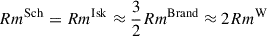 .
.
All Tables
All Figures
|
Fig. 1. Shape of b(ρ) for the Sharp (Eq. (26)) and Smooth (Eq. (28)) models for the same values of the parameters s, b∞, and Λ. |
| In the text | |
|
Fig. 2. Effective potential U(ρ) (Eq. (9)) that corresponds to the generation threshold for the two Sharp and two Smooth models. The length scale is normalized by the diffusion scale rd, which is taken to be the same for both models. The vertical arrows correspond to the δ functions in the Sharp model potential. |
| In the text | |
|
Fig. 3. Logarithmic derivative σ(ρ), Eq. (10), for the four models. The length scale is normalized by the same rd. The parameters of each model correspond to the generation threshold. |
| In the text | |
Current usage metrics show cumulative count of Article Views (full-text article views including HTML views, PDF and ePub downloads, according to the available data) and Abstracts Views on Vision4Press platform.
Data correspond to usage on the plateform after 2015. The current usage metrics is available 48-96 hours after online publication and is updated daily on week days.
Initial download of the metrics may take a while.