| Issue |
A&A
Volume 708, April 2026
|
|
|---|---|---|
| Article Number | A133 | |
| Number of page(s) | 9 | |
| Section | Numerical methods and codes | |
| DOI | https://doi.org/10.1051/0004-6361/202658989 | |
| Published online | 01 April 2026 | |
Numerical simulations of oscillating and differentially rotating neutron stars
1
Observatoire astronomique de Strasbourg, CNRS, Université de Strasbourg,
11 rue de l’Université,
67000
Strasbourg,
France
2
LUX, CNRS UMR 8262, Observatoire de Paris-PSL, Sorbonne Université Paris,
5 place Jules Janssen,
91190
Meudon,
France
★ Corresponding author: This email address is being protected from spambots. You need JavaScript enabled to view it.
Received:
15
January
2026
Accepted:
12
February
2026
Abstract
Context. The remnants of binary neutron star mergers are expected to be massive, rapidly rotating stars whose oscillations produce gravitational waves in the kilohertz band. The degree of differential rotation and the rotation profiles strongly influence their structure, stability, and oscillation spectrum, and must therefore be taken into account when modeling their dynamics.
Aims. We extend the pseudospectral code ROXAS (Relativistic Oscillations of non-aXisymmetric neutron stArS) to enable the dynamical evolution of oscillating, differentially rotating neutron stars. Using the updated code, we aim to study the star’s oscillation frequencies.
Methods. We extended the previous formalism, based on primitive variables and the conformal flatness approximation, to differential rotation. Within this framework, we ran a series of axisymmetric and nonaxisymmetric simulations of perturbed, differentially rotating neutron stars with different rotation rates, and extracted their oscillation frequencies.
Results. Axisymmetric modes, as well as those under the Cowling approximation, show excellent agreement with the published results. We show that the secondary fundamental mode in the Cowling approximation is an artifact that does not appear in dynamical space-times. In addition, we provide frequency values for nonaxisymmetric modes in differentially rotating configurations evolved in conformal flatness.
Conclusions. This extension broadens the range of physical scenarios that can be studied with ROXAS, and represents a step toward more realistic modeling of post-merger remnants and their gravitational-wave emission.
Key words: gravitation / gravitational waves / hydrodynamics / methods: numerical / stars: neutron / stars: oscillations (including pulsations)
© The Authors 2026
 Open Access article, published by EDP Sciences, under the terms of the Creative Commons Attribution License (https://creativecommons.org/licenses/by/4.0), which permits unrestricted use, distribution, and reproduction in any medium, provided the original work is properly cited.
This article is published in open access under the Subscribe to Open model. This email address is being protected from spambots. You need JavaScript enabled to view it. to support open access publication.
1 Introduction
The direct detection of gravitational waves (GWs), which started with the binary black hole merger GW150914 (Abbott et al. 2016), has opened a new window onto the most extreme astrophysical phenomena. Subsequently, the first GW signal from a binary neutron star (NS) merger, GW170817 (Abbott et al. 2017b), was observed together with its electromagnetic counterpart (Abbott et al. 2017a,c), which provided unprecedented insight into the dynamics of this system (Abbott et al. 2018). These detections were made possible by the current-generation GW detectors: the Laser Interferometer Gravitational-wave Observatory (LIGO) (Aasi et al. 2015), the Virgo GW detector (Acernese et al. 2015), and the Kamioka Gravitational-wave detector (KAGRA) (Akutsu et al. 2021).
From the first numerical simulations of the merger of two NSs (Shibata & Uryū 2000; Shibata et al. 2005), it is thought that in the majority of cases the post-merger remnant of a binary NS is a hypermassive neutron star (HMNS; Baumgarte et al. 2000), which is supported by its differential rotation for a few tenths of seconds. After that, the rotation slows down and becomes rigid, making this object collapse to a black hole (Metzger 2020). During this period, the HMNS is expected to emit GWs in the kilohertz frequency band, in a very similar manner to excited differentially rotating isolated NSs (Stergioulas et al. 2011). Thus, the study of the properties of differentially rotating NSs (see, e.g., recent works by Weih et al. 2018; Muhammed et al. 2024; Szewczyk et al. 2025) is very relevant to our understanding of binary NS mergers (Bauswein et al. 2016).
Note that current GW detectors lack sufficient sensitivity in the kilohertz band to detect the GWs from HMNS oscillations (Abbott et al. 2020). However, next-generation detectors such as the Einstein Telescope (Punturo et al. 2010), Cosmic Explorer (Reitze et al. 2019), and Neutron Star Extreme Matter Observatory (Ackley et al. 2020) will have a significantly increased sensitivity in this frequency range, where future detections could be a probe of the NS internal structure and its equation of state (EoS). In order to maximize the scientific output from these signals by the time they arrive, it is thus necessary to have a solid understanding of how the EoS, rotation, and other physical parameters shape the emitted GW.
To this end, the ROXAS code (Relativistic Oscillations of non-aXisymmetric neutron stArS; Servignat & Novak 2025; Servignat et al. 2025) was recently developed to evolve isolated NSs. It is a full nonlinear general-relativistic hydrodynamics code, primarily aimed at obtaining oscillation modes from these objects (see, e.g., Baiotti et al. 2009, for a comparison with linear approaches). It uses pseudospectral methods and a formulation based on primitive variables (Servignat et al. 2023) together with the extended conformal flatness (xCFC) formulation developed in Cordero-Carrión et al. (2009). The conformal flatness condition (CFC; Isenberg 2008; Wilson et al. 1996) has been proved to be a convenient approximation of full General Relativity (GR), which allows us to simplify the formalism while keeping a high degree of accuracy (Iosif & Stergioulas 2014). These approaches reduce the computational cost with respect to other codes that rely on conserved schemes (Banyuls et al. 1997; Cipolletta et al. 2020, 2021; Dimmelmeier et al. 2005, 2006; Thierfelder et al. 2011; Pakmor et al. 2016; Lioutas et al. 2024; Kidder et al. 2017; Rosswog & Diener 2021; Yamamoto et al. 2008), obtaining a lightweight code that can be run on office computers and is thus ideally suited for parametric studies. In this paper, we present an update of ROXAS that allows us to dynamically evolve perturbed, differentially rotating NSs. We describe the main changes to the formalism and code, and present a series of axisymmetric and nonaxisymmetric simulations of differentially rotating stars known as the B sequence (Stergioulas et al. 2004; Dimmelmeier et al. 2006; Krüger et al. 2010; Iosif & Stergioulas 2021), which use a polytropic EoS. We extract their oscillation modes and, when possible, compare their frequencies to those available in the literature for code validation, while the nonaxisymmetric ones in CFC are reported for the first time.
The article is structured as follows. In Sect. 2, we review the formalism used by ROXAS and stress the difference with differential rotation. In Sect. 3, we present the changes implemented in the code and detail the parameters used in our simulations. The results are discussed in Sect. 4, and finally conclusions with some final remarks are given in Sect. 5.
Unless otherwise stated, we use a geometrized unit system with G = c = 1 and a four-metric signature (−, +, +, +). Greek indices denote the four-dimensional space-time coordinates, while Latin ones represent the three-dimensional space. We also use Einstein’s summation convention over repeated indices.
2 Theoretical formalism
The formalism used here is based on the one in Servignat & Novak (2025) and Servignat et al. (2023), with some modifications to account for a differentially rotating star. The full details are provided in these references, and here we only summarize the main aspects and the key differences introduced in this paper.
2.1 Review of formalism
We considered a space-time described by the 3+1 formalism, so that the metric takes the form
![Mathematical equation: $\[g_{\mu v} d x^\mu d x^\nu=-N^2 d t^2+\gamma_{i j}(d x^i+\beta^i d t)(d x^j+\beta^j d t),\]$](/articles/aa/full_html/2026/04/aa58989-26/aa58989-26-eq1.png) (1)
(1)
where N is the lapse, βi the shift, and γij the induced spatial metric. We assumed CFC, so that
![Mathematical equation: $\[\gamma_{i j}=\Psi^4 f_{i j},\]$](/articles/aa/full_html/2026/04/aa58989-26/aa58989-26-eq2.png) (2)
(2)
where Ψ is called the conformal factor and fij is a flat metric. We denoted the covariant derivative associated with γij as Di and, as described by Bonazzola et al. (2004), we worked in maximal slicing and the Dirac gauge, which is automatically satisfied in CFC. The flat metric fij is expressed in spherical coordinates (r, θ, φ), as in Servignat & Novak (2025).
On the hydrodynamics side, we considered a simulated NS to be a perfect fluid, whose energy-momentum tensor is given by
![Mathematical equation: $\[T^{\mu \nu}=(e+p) u^\mu u^\nu+p g^{\mu \nu},\]$](/articles/aa/full_html/2026/04/aa58989-26/aa58989-26-eq3.png) (3)
(3)
where uμ is the time-like unitary four-velocity, e is the energy density in the fluid frame, and p is the pressure. The fluid is composed of baryons with a number density nB, at zero temperature, and in β equilibrium. The fluid thermodynamics can then be described by a barotropic EoS, p = p(nB), which we assume to be polytropic throughout this work, that is,
![Mathematical equation: $\[p=\kappa n_B^\gamma,\]$](/articles/aa/full_html/2026/04/aa58989-26/aa58989-26-eq4.png) (4)
(4)
where γ = 2 and κ = 0.02689 in LORENE units1, defined by c = r0 = m0 = 1, with r0 = 10 km and m0 ≈ 1.66 × 1029 kg. We also defined the log-enthalpy H,
![Mathematical equation: $\[H=\ln \left(\frac{e+p}{m_B n_B}\right),\]$](/articles/aa/full_html/2026/04/aa58989-26/aa58989-26-eq5.png) (5)
(5)
where mB ≈ 1.66 × 10⁻²⁷ kg is the nucleon mass. Additionally, we considered the Lorentz factor with respect to the Eulerian observer Γ, the Eulerian velocity of the fluid Ui, and its coordinate velocity vi, which satisfy the equations
![Mathematical equation: $\[\Gamma=\left(1-U_j U^j\right)^{-1 / 2},\]$](/articles/aa/full_html/2026/04/aa58989-26/aa58989-26-eq6.png) (6)
(6)
![Mathematical equation: $\[u^\alpha=\frac{\Gamma}{N}\left(1, v^i\right), \quad U^i=\frac{1}{N}\left(v^i+\beta^i\right).\]$](/articles/aa/full_html/2026/04/aa58989-26/aa58989-26-eq7.png) (7)
(7)
Within this framework, the basic evolution equations are (Servignat et al. 2023; Servignat & Novak 2025)
![Mathematical equation: $\[\begin{aligned}\partial_t H= & -v^i D_i H-c_s^2 \frac{\Gamma^2 N}{\Gamma^2-c_s^2\left(\Gamma^2-1\right)} \\& \times\left[K_{i j} U^i U^j+D_i U^i-\frac{U^i}{\Gamma^2} D_i H\right],\end{aligned}\]$](/articles/aa/full_html/2026/04/aa58989-26/aa58989-26-eq8.png) (8)
(8)
![Mathematical equation: $\[\begin{aligned}\partial_t U_i= & -v^j D_j U_i-U_j D_i v^j+N U_j D_i U^j-\frac{N}{\Gamma^2} D_i(H+\ln~ N) \\& +U_i U^j D_j N+\frac{c_s^2 N U_i}{\Gamma^2-c_s^2\left(\Gamma^2-1\right)} D_j U^j \\& +U_i \frac{\Gamma^2\left(c_s^2-1\right)}{\Gamma^2-c_s^2\left(\Gamma^2-1\right)} N U^l U^j K_{l j} \\& +\frac{\left(1-c_s^2\right) N}{\Gamma^2-c_s^2\left(\Gamma^2-1\right)} U_i U^j D_j H.\end{aligned}\]$](/articles/aa/full_html/2026/04/aa58989-26/aa58989-26-eq9.png) (9)
(9)
In a similar way to Servignat & Novak (2025), we decomposed each field into the equilibrium value, denoted with a subscript “eq”, plus the deviation of the total quantity from this equilibrium, denoted with a bar,
![Mathematical equation: $\[\begin{aligned}& U_i=U_{i, \mathrm{eq}}+\bar{U}_i, \quad H=H_{\mathrm{eq}}+\bar{H}, \\& \beta^i=\beta_{\mathrm{eq}}^i+\bar{\beta}^i, \quad N=N_{\mathrm{eq}}+\bar{N}.\end{aligned}\]$](/articles/aa/full_html/2026/04/aa58989-26/aa58989-26-eq10.png) (10)
(10)
Note that we did not assume that the latter quantities needed to be small.
The next step was to substitute these expressions into Eqs. (8) and (9), and use the identities satisfied at equilibrium to simplify the resulting equations. This is what we call “well-balanced formulation”, and where the main differences between rigid and differential rotation arise. This is not strictly speaking a well-balanced method as defined, for example, by Dumbser et al. (2024), but it is inspired by it.
2.2 Differential rotation
An axisymmetric star at equilibrium with an angular velocity, Ω(r, θ), so that ![Mathematical equation: $\[v_{\text {eq}}^{i}=\Omega(r, \theta) r ~\sin~ \theta \delta_{\varphi}^{i}\]$](/articles/aa/full_html/2026/04/aa58989-26/aa58989-26-eq11.png) , satisfies the equation (Bonazzola et al. 1993; Iosif & Stergioulas 2021)
, satisfies the equation (Bonazzola et al. 1993; Iosif & Stergioulas 2021)
![Mathematical equation: $\[H_{\mathrm{eq}}+\ln~ N_{\mathrm{eq}}-\ln~ \Gamma_{\mathrm{eq}}+\int_{\Omega_p}^{\Omega} F\left(\Omega^{\prime}\right) d \Omega^{\prime}=\mathrm{const}.,\]$](/articles/aa/full_html/2026/04/aa58989-26/aa58989-26-eq12.png) (11)
(11)
where
![Mathematical equation: $\[F=u^t u_{\varphi}=\frac{\Gamma_{\mathrm{eq}}^2}{N_{\mathrm{eq}}} U_{\varphi, \mathrm{eq}} r ~\sin~ \theta\]$](/articles/aa/full_html/2026/04/aa58989-26/aa58989-26-eq13.png) (12)
(12)
and Ωp is the angular velocity at the star’s pole.
The introduction of differential rotation thus involves the definition of a rotation law that relates these two variables, F(Ω). Historically, due to its simplicity, the most standard choice has been the Komatsu-Eriguchi-Hachisu (KEH) profile (Komatsu et al. 1989),
![Mathematical equation: $\[F(\Omega)=A^2\left(\Omega_c-\Omega\right),\]$](/articles/aa/full_html/2026/04/aa58989-26/aa58989-26-eq14.png) (13)
(13)
where Ωc is the central angular velocity and A is a constant that determines the length scale over which the angular velocity, Ω, changes. This can easily be seen in the Newtonian limit, where ut ≈ 1, gφφ ≈ (r sin θ)2 and uφ ≈ Ω, which yields the simple rotation law
![Mathematical equation: $\[\Omega(r, \theta)_{\mathrm{Newt}}=\frac{\Omega_c}{1+(r ~\sin~ \theta / A)^2}.\]$](/articles/aa/full_html/2026/04/aa58989-26/aa58989-26-eq15.png) (14)
(14)
In particular, A → ∞ corresponds to the rigidly rotating limit. The KEH profile produces a maximum frequency at the center of the star, which monotonically decreases with the radius, as can be seen in Fig. 3.
More recently, other differential rotation laws have been proposed that more realistically describe the situation in the post-merger remnant, such as those in Uryū et al. (2017). However, these profiles introduce additional computational challenges, as discussed in Sect. 3. In addition, for code validation purposes, it is useful to consider rotation profiles that have been more broadly studied in previous references. For these reasons, in the present paper, our numerical simulations only deal with KEH profiles, leaving more realistic and complex rotation laws for future work. In any case, the formalism described in this section remains general, with no particular assumption regarding the shape of F(Ω).
2.3 The well-balanced formulation with differential rotation
One of the main changes to obtaining hydrodynamics equations with differential rotation in the well-balanced formulation is the integral term that appears in Eq. (11). The other relevant identity that impacts the dynamical equations is
![Mathematical equation: $\[v_{\mathrm{eq}}^j D_j U_{i, \mathrm{eq}}+U_{j, \mathrm{eq}} D_i v_{\mathrm{eq}}^j=U_{\varphi, \mathrm{eq}} ~r ~\sin~ \theta D_i \Omega,\]$](/articles/aa/full_html/2026/04/aa58989-26/aa58989-26-eq16.png) (15)
(15)
with the right-hand side vanishing for rigid rotation. Both these equations produce additional terms in Eq. (9) with respect to the rigidly rotating case, leading to the final evolution equation for Ui:
![Mathematical equation: $\[\begin{aligned}\partial_t \bar{U}_i=&-\left[v_{\mathrm{eq}}^j D_j \bar{U}_i+\bar{v}^j D_j U_{i, \mathrm{eq}}+\bar{v}^j D_j \bar{U}_i\right.\\& +U_{j, \mathrm{eq}} D_i \bar{v}^j+\bar{U}_j D_i v_{\mathrm{eq}}^j+\bar{U}_j D_i \bar{v}^j \\& \left.-N\left(U_{j, \mathrm{eq}} D_i \bar{U}^j+\bar{U}_j D_i U_{\mathrm{eq}}^j+\bar{U}_j D_i \bar{U}^j\right)\right] \\& +N \bar{U}_j\left(2 U_{\mathrm{eq}}^j+\bar{U}^j\right) D_i\left(H_{\mathrm{eq}}+\ln~ N_{\mathrm{eq}}\right) \\& -\frac{N}{\Gamma^2} D_i\left(\bar{H}+\ln~ \left(1+\frac{\bar{N}}{N_{\mathrm{eq}}}\right)\right)+U_i U^j D_j N \\& +\frac{c_s^2 N U_i}{\Gamma^2-c_s^2\left(\Gamma^2-1\right)}\left(6 U_{\mathrm{eq}}^{\varphi} \bar{D}_{\varphi} ~\ln~ \Psi+D_j \bar{U}^j\right) \\& +U_i \frac{\Gamma^2\left(c_s^2-1\right)}{\Gamma^2-c_s^2\left(\Gamma^2-1\right)} N U^l U^j K_{l j} \\& +\frac{\left(1-c_s^2\right) N}{\Gamma^2-c_s^2\left(\Gamma^2-1\right)} U_i U^j D_j H \\& +\frac{\bar{N}}{N_{\mathrm{eq}}} U_{\varphi, \mathrm{eq}} ~r ~\sin~ \theta ~D_i \Omega,\end{aligned}\]$](/articles/aa/full_html/2026/04/aa58989-26/aa58989-26-eq17.png) (16)
(16)
where the last term is a combination of the two described contributions from differential rotation. Two additional terms appear that were not present in Servignat & Novak (2025), corresponding to higher-order contributions that do not contribute to the evolution in a relevant way in most cases. However, it is safer to account for them, especially for high velocities or if large deviations from equilibrium are involved.
Regarding the equation for the enthalpy, Eq. (8) can be slightly simplified by using the same identity used for rigid rotation, ![Mathematical equation: $\[v_{\text {eq}}^{i} D_{i} H_{\text {eq }}=0\]$](/articles/aa/full_html/2026/04/aa58989-26/aa58989-26-eq18.png) , leading to the same evolution equation for H:
, leading to the same evolution equation for H:
![Mathematical equation: $\[\begin{aligned}\partial_t \bar{H} & =-\bar{v}^i D_i H_{\mathrm{eq}}-v_{\mathrm{eq}}^i D_i \bar{H}-\bar{v}^i D_i \bar{H} \\-c_s^2 & \frac{\Gamma^2 N}{\Gamma^2-c_s^2\left(\Gamma^2-1\right)}\left[K_{i j} U^i U^j-K+D_i U^i-\frac{U^i}{\Gamma^2} D_i H\right].\end{aligned}\]$](/articles/aa/full_html/2026/04/aa58989-26/aa58989-26-eq19.png) (17)
(17)
3 Numerical simulations
The numerical simulations performed in this work were performed with a modified version of the code ROXAS (Servignat & Novak 2025)2. The changes made to the code – mainly motivated by the introduction of differential rotation – are summarized below.
3.1 Updates to the code
ROXAS is a pseudospectral code for the dynamical evolution of perturbed, isolated rotating NSs. It makes use of the LORENE (Langage Objet pour la RElativité NumériquE; Gourgoulhon et al. 2016) infrastructure and, in particular, it relies on it to produce the equilibrium star that is perturbed and evolved. Therefore, differential rotation needs to be implemented in both LORENE and ROXAS.
Although tools for computing the equilibrium configuration of a differentially rotating star have been previously implemented in LORENE (Saijo & Gourgoulhon 2006), these solvers were based on the full GR formalism. We implemented new solvers under the CFC assumption, which reduces the number of metric variables and simplifies the system of Einstein equations to be solved.
Despite the fact that we focus on KEH rotation profiles throughout this text, the goal is to be able to use more complex profiles in the future. Profiles such as those in Uryū et al. (2017) need to be specified through a noninjective function Ω(F), which cannot be inverted as F(Ω). While KEH profiles are generally defined through the F(Ω) in Eq. (13), this relation can be inverted and also expressed as an Ω(F),
![Mathematical equation: $\[\Omega(F)=\Omega_c-\frac{F}{A^2}.\]$](/articles/aa/full_html/2026/04/aa58989-26/aa58989-26-eq20.png) (18)
(18)
With this change, the integral term in the equilibrium equation, Eq. (11), needs to be computed as
![Mathematical equation: $\[\int_{F_p}^F F^{\prime} \frac{d \Omega}{d F}\left(F^{\prime}\right) d F^{\prime},\]$](/articles/aa/full_html/2026/04/aa58989-26/aa58989-26-eq21.png) (19)
(19)
but otherwise the formalism remains the same. As using Ω(F) is therefore a more generic framework, we chose this way to define the rotation profile for our implementation, in contrast to the original implementation of differential rotation in LORENE.
Note that this step alone is insufficient to deal with the profiles in Uryū et al. (2017), since other challenges remain. For instance, these profiles involve a higher number of free parameters whose values are usually determined through other variables with more clear physical meanings, as can be seen in Iosif & Stergioulas (2021). This implies that these parameters change during the iterative process to find the star’s equilibrium configuration, possibly leading to the algorithm failing or to nonphysical configurations if not treated carefully, especially in the most rapidly rotating cases. Another issue is that these profiles show a local maximum in the angular velocity at a nonzero radius, contrary to KEH profiles (see Fig. 3), which requires more resolution around this point in the dynamical evolution and usually leads to less stable simulations.
Once a NS equilibrium configuration is found, the resulting fields are stored for later usage with ROXAS, including Ω (for use in Eq. (16), for example) instead of F, which can be recovered from other variables. ROXAS was also modified to read equilibrium configurations of differentially rotating stars, as well as to account for the additional terms described in Sect. 2 for a consistent dynamical evolution. Before evolving the star, a perturbation is added to either the Eulerian velocity, Ui, or to the log-enthalpy, H. In the latter case, the perturbation can be chosen to be
![Mathematical equation: $\[\delta H=\varepsilon\left(x^2 \pm y^2-\frac{2}{3} r^2\right)\left(1-\frac{r^2}{R_S(\theta)^2}\right),\]$](/articles/aa/full_html/2026/04/aa58989-26/aa58989-26-eq22.png) (20)
(20)
where RS(θ) is the radius of the equilibrium star in the direction of θ. In this equation, the minus sign (−) corresponds to a nonaxisymmetric perturbation that mixes l = m = 0 and l = m = 2 modes, as defined and used in Servignat & Novak (2025), while the plus sign (+) yields axial symmetry, which is useful for saving simulation time if only an axisymmetric study is required.
Finally, ROXAS is now able to export one-dimensional profiles and two-dimensional slices of the hydrodynamic and metric grids during the simulation, where the output rate can be specified independently. They can easily be plotted afterwards, and allow us to have a better understanding of how the simulation internally behaves, and to spot potential issues. Examples with the initial profile and slice of the enthalpy perturbation of a nonaxisymmetric simulation are shown in Figs. 1 and 2, respectively.
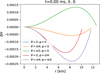 |
Fig. 1 Radial profile in different directions of the initial enthalpy perturbation of the nonaxisymmetric B4 simulations. |
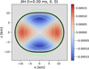 |
Fig. 2 Slice in the xz plane of the initial enthalpy perturbation of the nonaxisymmetric B4 simulations. The dashed green lines correspond to the boundaries between the different domains of the metric grid, as described in Sect. 3.2. |
3.2 Simulation parameters
In order to test the new implemented changes, we checked the consistency with other numerical simulations of oscillations in differentially rotating stars in the literature. In particular, we used the B sequence described in Dimmelmeier et al. (2006) and compared the resulting frequencies with those provided in this reference.
For the B sequence, the central value for the log-enthalpy is the same as in the BU sequence used in Servignat & Novak (2025), which in LORENE units is Hc = 0.2280. For the rotation profile in Eq. (13), we set A = re, with re being the star radius at the equator. The B sequence is defined by the star’s flattening (ratio between the star’s radius at the pole, rp, and re). However, LORENE does not take this as an input parameter, and requires the central angular velocity Ωc. Therefore, we took these values from Dimmelmeier et al. (2006) and checked that the final configurations found by the algorithm yielded similar values of rp/re, masses, and ratios between kinetic and potential energies, T/W. A summary of these parameters and their relative errors with respect to those in Dimmelmeier et al. (2006) is provided in Table 1. We can see that the agreement is excellent, even for the fastest rotating stars. The largest errors correspond to T/W for B1 and B2, due to the smallness of these quantities compared to the precision of the reference values.
With respect to the dynamical evolution with ROXAS, the simulation properties are very similar to the ones in Servignat & Novak (2025). Two types of grids are used, with the following parameters:
The hydro grid consists of two domains: the spherical nucleus, with a maximum radius of 0.7 rp, and a shell that covers the rest of the star. In both domains, we set Nr = Nθ = 17, with Ni, i = r, θ, φ, the number of grid points for each coordinate. In addition, Nφ is set to 8 for the nonaxisymmetric simulations and to 1 for the axisymmetric ones. In Servignat & Novak (2025), Nθ is increased for the most demanding (i.e., more rapidly rotating) simulations, but we found them to be more stable by keeping the same value;
The metric grid consists of several spherical domains: a nucleus that extends up to 8 km (7 km for B9, which has rp ≈ 7.5 km), a first shell from this radius up to rp, four more shells up to re, and then one more up to 20 km followed by the compactified external domain, in which a change in variable u = 1/r is made to take into account boundary conditions at r → ∞ (Bonazzola et al. 1998). The four shells between rp and re are chosen so that their edges match RS(θ) for θ uniformly spaced between 0 and π/2.
Physical parameters of the computed NS equilibrium configurations.
4 Results
We carried out an initial test of the code to check its ability to keep stable equilibrium initial data, with the evolution of unperturbed differentially rotating NS. Some angular velocity profiles corresponding to an unperturbed B4 are thus shown in Fig. 3, both initially and after a dynamical evolution in CFC of 25 ms. The fact that these profiles remain constant after this time period (many rotation periods) shows that the formalism, the dynamical code, and the equilibrium star solvers work together consistently and in a stable way.
Then, for each of the differentially rotating NSs in equilibrium reported in Table 1, we performed four simulations: two in the Cowling approximation and another two with dynamical space-time under CFC. For each pair, one of the simulations is evolved in axisymmetry after adding an axisymmetric perturbation of the form (20) (+ sign) to the equilibrium star, while the other one is evolved in 3D3 after adding a nonaxisymmetric perturbation of the form (20) (− sign). In all cases, the amplitude is chosen to be ϵ = 10−3 in code units. The GWs were extracted following the procedure in Servignat & Novak (2025), based on Einstein’s quadrupole formula; an example waveform is provided in Fig. 6.
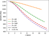 |
Fig. 3 Angular velocity profiles in different directions for an unperturbed B4 simulation. The solid lines correspond to the initial profiles, while the superimposed points are plotted after 25 ms of dynamical evolution in CFC. |
4.1 Cowling approximation
The Cowling approximation assumes that the metric stays static and equal to the values at equilibrium. This approximation has been widely used for the simulation of relativistic stars (see, e.g., McDermott et al. 1983; Villain & Bonazzola 2002; Sotani et al. 2023; Montefusco et al. 2025) due to the reduction in the computational cost of simulations. While this is not particularly relevant for ROXAS, running some simulations in the Cowling approximation allows us to perform more extensive code validation against existing literature. In particular, axisymmetric modes can be compared to those in Stergioulas et al. (2004), which used an axisymmetric code for dynamical evolution in GR under the Cowling approximation. On the other hand, nonaxisymmetric modes can be compared to Krüger et al. (2010), where these frequencies were obtained with a perturbative approach, once again limited to the Cowling approximation.
When possible, these simulations were run for 25 ms; however, for the most demanding configurations, the nonaxisymmetric simulations are only stable up to shorter times, which are reported in Table 2. In these cases, at late stages, the fields develop unphysical, large, high-order coefficients in the spectral representation, leading to an eventual numerical crash, without preceding signatures of physical instabilities such as shock formation. Possible causes include insufficient resolution or aliasing effects; we will investigate these further and attempt to mitigate them in future works.
An example frequency spectrum for the nonaxisymmetric B4 simulation is provided in Fig. 4, where we can distinguish the different oscillation modes present in the simulation. In particular, a secondary fundamental mode, FII, appears around 2.6 kHz, as was reported for the first time in Stergioulas et al. (2004). As FII and 2f−2 have similar values, they generate a single joint peak in Fig. 4. However, this secondary fundamental mode can be identified independently in the absence of an 2f−2, such as in axisymmetric simulations or in spectra corresponding to l = m = 0 modes, as in Fig. 5 presented in the next subsection.
The frequencies for the full B sequence are presented in Table 2, where the precise values are extracted from the Fourier transform of the decomposition of the star’s radius, RS, into spherical harmonics. These time series include fewer oscillation modes per multipole order, leading to more isolated and cleaner peaks and, therefore, to a more precise frequency determination.
The axisymmetric frequencies we extracted are the fundamental modes F and FII, their first overtone H1, the l = 2, m = 0 mode 2f0, and its first overtone 2p1. The values shown in Table 2 correspond to those obtained from the axisymmetric simulations, given their better stability and lower number of modes, which generate cleaner peaks. However, as these frequencies are also present in the nonaxisymmetric simulations, we extracted them from these simulations as well, and obtained the same values up to maximum relative errors of 0.9%. On the other hand, the extracted nonaxisymmetric frequencies are the l = |m| = 2 modes, denoted by 2f2 and 2f−2, and appear only in the nonaxisymmetric simulations.
The relative errors of our results with respect to Stergioulas et al. (2004) and Krüger et al. (2010) are provided in Table 2. Most of them are similar or below 2%. The larger values of δ2f2 from B6 on can be explained by the smallness of these frequencies compared to our frequency resolution. Similarly, the 3.16% error in FII for B2 is due to the fact that the peaks for F and FII are completely blended in our B2 spectrum, which leads us to report them as equal.
Mode frequencies (in kilohertz) from the B sequence simulations in the Cowling approximation.
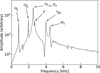 |
Fig. 4 Gravitational waves spectrum of the nonaxisymmetric B4 simulation in the Cowling approximation. |
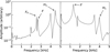 |
Fig. 5 Fourier spectrum of the l = m = 0 RS coefficient for the nonaxisymmetric B4 simulation in the Cowling approximation (left) and a dynamical space-time (right). |
Mode frequencies (kilohertz) from the B sequence simulations in CFC.
4.2 Full dynamics in CFC
Having checked that ROXAS produces consistent results with other articles within the Cowling approximation, we were able to relax this assumption and work with the Einstein-CFC system solved dynamically (see Servignat & Novak (2025) for details), using the full potential of the code. In this case, the waveform spectra show a single fundamental mode, unlike the double peak seen in the Cowling approximation. We can see this more clearly by comparing the spectra of the l = m = 0 coefficient of RS, from which the fundamental frequencies and their overtones are extracted, as can be seen in Fig. 5. In this figure, we can see the two fundamental-mode peaks around 2.6 kHz in the Cowling simulation, while there is a single fundamental-mode peak around 1.3 kHz in the CFC simulation. This confirms that the secondary fundamental mode is an artifact of the Cowling approximation in differential rotation, as was suspected in Stergioulas et al. (2004). While previous works such as Dimmelmeier et al. (2006) studied axisymmetric modes without the Cowling approximation, this is the first time this difference is explicitly addressed by comparing both types of simulation.
We show an example waveform in Fig. 6, with its spectrum in Fig. 7, that corresponds to the nonaxisymmetric B4 simulation in CFC. In Table 3, we report the frequencies for the same axisymmetric and nonaxisymmetric modes as those described in the previous section, this time for the B sequence in a dynamical space-time. The only exception is the secondary fundamental mode, which is absent in this case. Once again, the axisymmetric modes in Table 3 correspond to the axisymmetric simulations, while we use the nonaxisymmetric ones to check the consistency of these modes and to extract the nonaxisymmetric frequencies. The maximum relative error between the axisymmetric modes of both types of simulation is 6.5%, which corresponds to H1 for B9. This is an outlier caused by a higher-frequency peak (≈4.45 kHz), which merges with the one corresponding to H1 in the nonaxisymmetric simulation. Both of them can be resolved in the axisymmetric simulation, as would likely be the case with a longer nonaxisymmetric simulation. Other than that, the largest relative error is 2.4%.
The nonaxisymmetric modes are reported here for the first time, to our knowledge. The 2f2 frequency becomes negative from B7 onward, indicating that this mode rotates in the opposite direction with respect to the previous cases, in the star’s co-rotating reference frame. For low rotation frequencies, the (2, 2) mode corresponds to a prograde rotation, while the (2, −2) is retrograde. The regime where the (2, 2) mode is also retrograde is called the CFS (Chandrasekhar-Friedman-Schutz) instability (Chandrasekhar 1970; Friedman & Schutz 1978; Friedman & Schutz 1978), as reported in Krüger et al. (2010) within the Cowling approximation and in Zink et al. (2010) and Krüger & Kokkotas (2020) for rigid rotation. With our approach, both rotation directions can be distinguished with a Fourier transform of the complex l = m = 2 RS coefficient. We can see the different behaviors in Fig. 8.
On the other hand, the axisymmetric modes can be compared to the values quoted in Dimmelmeier et al. (2006), in which axisymmetric, dynamical simulations were performed in CFC. The relative errors between this work and ours are also included in Table 3.
We can see that the agreement of H1, 2f0, and 2p1 is of the order of 1% or lower in most of the cases. For the H1 corresponding to B9, a similar issue to ours might have also arisen in Dimmelmeier et al. (2006), as their reported frequency is closer to the misleading 4.45 kHz found in our simulations, which leads to a similar relative error of 6.5%. The fundamental frequency, F, however, shows larger discrepancies, especially in the fastest rotating cases. Taking into account the uncertainties purely associated with the frequency resolution limited by the total simulation time (see Fig. 9), there is only a clear tension for the B7 and B9 simulations. However, the fundamental frequencies in Dimmelmeier et al. (2006) show a faster decaying trend than ours. The origin of these discrepancies is unclear at this point, as the codes, resolutions, and simulation times of both works are different, which requires a more detailed investigation. Note that the CFC approximation, which is also used in Dimmelmeier et al. (2006), is not the cause. While a comparison with frequencies obtained directly from GR is not possible here, it was done for the rigidly rotating case in Servignat & Novak (2025) with excellent agreement, showing the reliability of CFC for NS oscillation-mode studies.
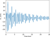 |
Fig. 6 Gravitational wave strain extracted from the nonaxisymmetric B4 simulation in CFC. |
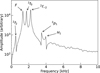 |
Fig. 7 Gravitational wave spectrum of the nonaxisymmetric B4 simulation in CFC. |
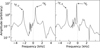 |
Fig. 8 Fourier spectrum of the complex l = m = 2 RS coefficient for the nonaxisymmetric B4 (left) and B8 (right) simulations in CFC. |
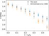 |
Fig. 9 Fundamental frequencies obtained for the B sequence simulations and comparison with those in Dimmelmeier et al. (2006). The error bars are the inverse of the simulation times, which correspond to the frequency resolutions. |
5 Conclusions
In this work, we present an update of the publicly available code ROXAS, which can now simulate differentially rotating stars, together with several additional improvements. We ran a series of both nonaxisymmetric and axisymmetric simulations, first in the Cowling approximation and then with a dynamical space-time in CFC. We verified their consistency with different references and obtained excellent overall agreement for both axisymmetric and nonaxisymmetric mode frequencies. In addition, we show that, as conjectured in Stergioulas et al. (2004), the secondary fundamental peak appearing in simulations within the Cowling approximation does not appear in dynamical space-times under the same initial conditions.
Furthermore, the nonaxisymmetric frequencies 2f2 and 2f−2 in CFC are reported here for the first time, illustrating the ability of ROXAS to explore a wider class of configurations and generate novel results. We also emphasize that these simulations are performed with a lightweight code that runs efficiently on standard computers within short computation times, even though it is not parallel. For radial (one-dimensional) simulations, ROXAS typically performs about five times faster (Servignat et al. 2023) than the reference core-collapse and NS oscillation code CoCoNuT (Dimmelmeier et al. 2005) used in its sequential version. Assuming that this improvement scales equally in all dimensions and no paralellization, this effect should be enhanced for axisymmetric (giving roughly a factor of 52 = 25) and nonaxisymmetric (a factor of 53 = 125) simulations. Nevertheless, these are order-of-magnitude estimates and a direct comparison through benchmarking of multi-dimensional simulations remains to be done in order to properly assess the difference in performance.
Together with Servignat & Novak (2025), this work represents an initial step toward a versatile tool for studying perturbed, rotating NSs with moderate computational resources. Building on this, future works will include differential rotation profiles, which are more motivated by binary NS simulations, such as those in Uryū et al. (2017), as well as more realistic EoSs, which will require further extensions of the present framework.
Acknowledgements
The authors acknowledge support from the Agence Nationale de la Recherche (ANR) under contract ANR-22-CE31-0001-01.
References
- Aasi, J. et al. 2015, Class. Quant. Grav., 32, 074001 [Google Scholar]
- Abbott, B. P. et al. 2016, Phys. Rev. Lett., 116, 061102 [CrossRef] [PubMed] [Google Scholar]
- Abbott, B. P. et al. 2017a, Astrophys. J. Lett., 848, L13 [CrossRef] [Google Scholar]
- Abbott, B. P. et al. 2017b, Phys. Rev. Lett., 119, 161101 [CrossRef] [Google Scholar]
- Abbott, B. P. et al. 2017c, Astrophys. J. Lett., 848, L12 [CrossRef] [Google Scholar]
- Abbott, B. P. et al. 2018, Phys. Rev. Lett., 121, 161101 [NASA ADS] [CrossRef] [Google Scholar]
- Abbott, B. P. et al. 2020, Living Rev. Rel., 23, 3 [Google Scholar]
- Acernese, F. et al. 2015, Class. Quant. Grav., 32, 024001 [NASA ADS] [CrossRef] [Google Scholar]
- Ackley, K., Adya, V. B., Agrawal, P., et al. 2020, Publ. Astron. Soc. Aust., 37, e047 [Google Scholar]
- Akutsu, T. et al. 2021, PTEP, 2021, 05A101 [Google Scholar]
- Baiotti, L., Bernuzzi, S., Corvino, G., de Pietri, R., & Nagar, A. 2009, Phys. Rev. D, 79, 024002 [Google Scholar]
- Banyuls, F., Font, J. A., Ibáñez, J. M. A., Martí, J. M. A., & Miralles, J. A. 1997, Astrophys. J., 476, 221 [Google Scholar]
- Baumgarte, T. W., Shapiro, S. L., & Shibata, M. 2000, Astrophys. J. Lett., 528, L29 [Google Scholar]
- Bauswein, A., Stergioulas, N., & Janka, H.-T. 2016, Eur. Phys. J. A, 52, 56 [NASA ADS] [CrossRef] [Google Scholar]
- Bonazzola, S., Gourgoulhon, E., Salgado, M., & Marck, J. A. 1993, Astron. Astrophys., 278, 421 [Google Scholar]
- Bonazzola, S., Gourgoulhon, E., & Marck, J.-A. 1998, Phys. Rev. D, 58, 1 [CrossRef] [Google Scholar]
- Bonazzola, S., Gourgoulhon, E., Grandclément, P., & Novak, J. 2004, Phys. Rev. D, 70, 1 [Google Scholar]
- Chandrasekhar, S. 1970, Astrophys. J., 161, 561 [Google Scholar]
- Cipolletta, F., Kalinani, J. V., Giacomazzo, B., & Ciolfi, R. 2020, Class. Quant. Grav., 37, 135010 [Google Scholar]
- Cipolletta, F., Kalinani, J. V., Giangrandi, E., et al. 2021, Class. Quant. Grav., 38, 085021 [Google Scholar]
- Cordero-Carrión, I., Cerda-Durán, P., Dimmelmeier, H., et al. 2009, Phys. Rev. D, 79, 024017 [CrossRef] [Google Scholar]
- Dimmelmeier, H., Novak, J., Font, J. A., Ibáñez, J. M., & Müller, E. 2005, Phys. Rev. D, 71, 064023 [Google Scholar]
- Dimmelmeier, H., Stergioulas, N., & Font, J. A. 2006, Mon. Not. Roy. Astron. Soc., 368, 1609 [Google Scholar]
- Dumbser, M., Zanotti, O., Gaburro, E., & Peshkov, I. 2024, J. Computat. Phys., 504, 112875 [Google Scholar]
- Friedman, J. L., & Schutz, B. F. 1978, Astrophys. J., 221, 937 [Google Scholar]
- Friedman, J. L., & Schutz, B. F. 1978, Astrophys. J., 222, 281 [Google Scholar]
- Gourgoulhon, É., Grandclément, P., Marck, J.-A., Novak, J., & Taniguchi, K. 2016, LORENE: Spectral methods differential equations solver, Astrophysics Source Code Library [record ascl:1608.018] [Google Scholar]
- Iosif, P., & Stergioulas, N. 2014, Gen. Rel. Grav., 46, 1800 [Google Scholar]
- Iosif, P., & Stergioulas, N. 2021, Mon. Not. Roy. Astron. Soc., 503, 850 [Google Scholar]
- Isenberg, J. A. 2008, Int. J. Mod. Phys. D, 17, 265 [NASA ADS] [CrossRef] [Google Scholar]
- Kidder, L. E. et al. 2017, J. Comput. Phys., 335, 84 [Google Scholar]
- Komatsu, H., Eriguchi, Y., & Hachisu, I. 1989, Mon. Not. Roy. Astron. Soc., 237, 355 [Google Scholar]
- Krüger, C., Gaertig, E., & Kokkotas, K. D. 2010, Phys. Rev. D, 81, 084019 [Google Scholar]
- Krüger, C. J., & Kokkotas, K. D. 2020, Phys. Rev. D, 102, 064026 [Google Scholar]
- Lioutas, G., Bauswein, A., Soultanis, T., et al. 2024, Mon. Not. Roy. Astron. Soc., 528, 1906 [Google Scholar]
- McDermott, P. N., van Horn, H. M., & Scholl, J. F. 1983, Astrophys. J., 268, 837 [Google Scholar]
- Metzger, B. D. 2020, Living Rev. Rel., 23, 1 [Google Scholar]
- Montefusco, G., Antonelli, M., & Gulminelli, F. 2025, Astron. Astrophys., 694, A150 [Google Scholar]
- Muhammed, N., Duez, M. D., Chawhan, P., et al. 2024, Phys. Rev. D, 110, 124063 [Google Scholar]
- Pakmor, R., Springel, V., Bauer, A., et al. 2016, Mon. Not. Roy. Astron. Soc., 455, 1134 [Google Scholar]
- Punturo, M. et al. 2010, Class. Quant. Grav., 27, 194002 [Google Scholar]
- Reitze, D. et al. 2019, Bull. Am. Astron. Soc., 51, 035 [Google Scholar]
- Rosswog, S., & Diener, P. 2021, Class. Quant. Grav., 38, 115002 [Google Scholar]
- Saijo, M., & Gourgoulhon, É. 2006, Phys. Rev. D, 74, 084006 [Google Scholar]
- Servignat, G., & Novak, J. 2025, Class. Quant. Grav., 42, 095015 [Google Scholar]
- Servignat, G., Novak, J., & Cordero-Carrión, I. 2023, Class. Quant. Grav., 40, 105002 [Google Scholar]
- Servignat, G., Novak, J., & Jaraba, S. 2025, ROXAS [Google Scholar]
- Shibata, M., & Uryū, K. 2000, Phys. Rev. D, 61, 1 [Google Scholar]
- Shibata, M., Taniguchi, K., & Uryū, K. 2005, Phys. Rev. D, 71, 084021 [Google Scholar]
- Sotani, H., Kokkotas, K. D., & Stergioulas, N. 2023, Astron. Astrophys., 676, A65 [Google Scholar]
- Stergioulas, N., Apostolatos, T. A., & Font, J. A. 2004, Mon. Not. Roy. Astron. Soc., 352, 1089 [Google Scholar]
- Stergioulas, N., Bauswein, A., Zagkouris, K., & Janka, H.-T. 2011, Mon. Not. Roy. Astron. Soc., 418, 427 [Google Scholar]
- Szewczyk, P., Gondek-Rosińska, D., & Cerdá-Durán, P. 2025, Astrophys. J., 990, 199 [Google Scholar]
- Thierfelder, M., Bernuzzi, S., & Bruegmann, B. 2011, Phys. Rev. D, 84, 044012 [Google Scholar]
- Uryū, K., Tsokaros, A., Baiotti, L., et al. 2017, Phys. Rev. D, 96, 103011 [Google Scholar]
- Villain, L., & Bonazzola, S. 2002, Phys. Rev. D, 66, 123001 [Google Scholar]
- Weih, L. R., Most, E. R., & Rezzolla, L. 2018, Mon. Not. Roy. Astron. Soc., 473, L126 [Google Scholar]
- Wilson, J. R., Mathews, G. J., & Marronetti, P. 1996, Phys. Rev. D, 54, 1317 [Google Scholar]
- Yamamoto, T., Shibata, M., & Taniguchi, K. 2008, Phys. Rev. D, 78, 064054 [Google Scholar]
- Zink, B., Korobkin, O., Schnetter, E., & Stergioulas, N. 2010, Phys. Rev. D, 81, 084055 [Google Scholar]
This corresponds to the standard polytropic EoS in, for example, Stergioulas et al. (2004) and Dimmelmeier et al. (2006), where p = κρργ, with ρ= mBnB, γ = 2, and κρ = 100 in the geometrized unit system supplemented with M⊙ = 1.
The version with rigid rotation was made publicly available in Servignat et al. (2025) in February 2025.
We imposed symmetries with respect to the equatorial plane and by rotating π around the vertical z axis. These symmetries include the dominant quadrupolar ℓ = |m| = 2 mode (see Servignat & Novak 2025).
All Tables
Mode frequencies (in kilohertz) from the B sequence simulations in the Cowling approximation.
All Figures
|
Fig. 1 Radial profile in different directions of the initial enthalpy perturbation of the nonaxisymmetric B4 simulations. |
| In the text | |
|
Fig. 2 Slice in the xz plane of the initial enthalpy perturbation of the nonaxisymmetric B4 simulations. The dashed green lines correspond to the boundaries between the different domains of the metric grid, as described in Sect. 3.2. |
| In the text | |
|
Fig. 3 Angular velocity profiles in different directions for an unperturbed B4 simulation. The solid lines correspond to the initial profiles, while the superimposed points are plotted after 25 ms of dynamical evolution in CFC. |
| In the text | |
|
Fig. 4 Gravitational waves spectrum of the nonaxisymmetric B4 simulation in the Cowling approximation. |
| In the text | |
|
Fig. 5 Fourier spectrum of the l = m = 0 RS coefficient for the nonaxisymmetric B4 simulation in the Cowling approximation (left) and a dynamical space-time (right). |
| In the text | |
|
Fig. 6 Gravitational wave strain extracted from the nonaxisymmetric B4 simulation in CFC. |
| In the text | |
|
Fig. 7 Gravitational wave spectrum of the nonaxisymmetric B4 simulation in CFC. |
| In the text | |
|
Fig. 8 Fourier spectrum of the complex l = m = 2 RS coefficient for the nonaxisymmetric B4 (left) and B8 (right) simulations in CFC. |
| In the text | |
|
Fig. 9 Fundamental frequencies obtained for the B sequence simulations and comparison with those in Dimmelmeier et al. (2006). The error bars are the inverse of the simulation times, which correspond to the frequency resolutions. |
| In the text | |
Current usage metrics show cumulative count of Article Views (full-text article views including HTML views, PDF and ePub downloads, according to the available data) and Abstracts Views on Vision4Press platform.
Data correspond to usage on the plateform after 2015. The current usage metrics is available 48-96 hours after online publication and is updated daily on week days.
Initial download of the metrics may take a while.