| Issue |
A&A
Volume 709, May 2026
|
|
|---|---|---|
| Article Number | A178 | |
| Number of page(s) | 6 | |
| Section | Planets, planetary systems, and small bodies | |
| DOI | https://doi.org/10.1051/0004-6361/202556405 | |
| Published online | 13 May 2026 | |
Galactic trajectories of interstellar objects 1I/’Oumuamua, 2I/Borisov, and 3I/ATLAS
Astronomy Department, Harvard University,
60 Garden St.,
Cambridge,
MA
02138,
USA
★ Corresponding authors: This email address is being protected from spambots. You need JavaScript enabled to view it.
; This email address is being protected from spambots. You need JavaScript enabled to view it.
Received:
14
July
2025
Accepted:
11
February
2026
Abstract
Aims. The first interstellar objects, 1I/’Oumuamua, 2I/Borisov, and 3I/ATLAS, were discovered over the past decade.
Methods. We follow the trajectories of known interstellar objects in the gravitational potential of the Milky Way galaxy to constrain their possible origin.
Results. We performed Monte Carlo orbital integrations using an ensemble of 10 000 trajectories per object to propagate measurement uncertainties in both object velocities and solar motion parameters through a Milky Way potential. We then used a Bayesian statistical framework that combines the resulting distributions of maximum vertical excursion (zmax) with age-velocity-dispersion relations and star-formation-rate priors to infer plausible stellar ages.
Conclusions. Our Monte Carlo analysis yields median zmax values of 0.016 ± 0.002 kpc for 1I/’Oumuamua, 0.121 ± 0.010 kpc for 2I/Borisov, and 0.481−0.017+0.023 kpc for 3IZATLAS. The Bayesian age inference indicates that 1I/’Oumuamua originated from a young stellar system (3.2 Gyr, 68% credible interval (CI): 0.5-8.8 Gyr), 2I/Borisov from an intermediate-age population (5.0 Gyr, 68% CI: 1.8-9.7 Gyr), and 3IZATLAS from an old thick-disk source (8.7 Gyr, 68% CI: 5.2-10.3 Gyr). Taken together, these estimates are consistent with smaller vertical excursions tracing younger parent populations under our stated kinematic assumptions.
Key words: comets: general / minor planets, asteroids: general / comets: individual: 1I/’Oumuamua / comets: individual: 2I/Borisov / comets: individual: 3I/ATLAS
© The Authors 2026
 Open Access article, published by EDP Sciences, under the terms of the Creative Commons Attribution License (https://creativecommons.org/licenses/by/4.0), which permits unrestricted use, distribution, and reproduction in any medium, provided the original work is properly cited.
This article is published in open access under the Subscribe to Open model. This email address is being protected from spambots. You need JavaScript enabled to view it. to support open access publication.
1 Introduction
The discovery of interstellar objects over the past decade has sparked significant interest in their origins and dynamics (see reviews by Siraj & Loeb (2022a), Jewitt & Seligman (2023), Jewitt (2024), and references therein). 1I/’Oumuamua was first reported in late 2017 (Meech et al. 2017; Williams 2017), and 2IZBorisov (C/2019 Q4) was identified in 2019 as an interstellar comet (Guzik et al. 2020). The more recent object, 3IZATLAS (CZ2025 N1), has been analyzed in subsequent kinematic studies (Seligman et al. 2025; Taylor & Seligman 2025). A fundamental question is the origin of each of these objects (Bailer-Jones et al. 2018; Bailer-Jones et al. 2020). Constraining their sources can shed light on the nature of these interstellar objects and the astrophysical processes that created them (see, e.g., Zhang & Lin 2020 and Loeb & MacLeod 2024).
In this paper, we numerically integrated the trajectories of interstellar objects backward in time in the gravitational potential of the Milky Way to relate them to potential stellar populations. We briefly review related work on kinematic age inference and backtracking (e.g., Almeida-Fernandes & Rocha-Pinto 2018; Hallatt & Wiegert 2020; Hsieh et al. 2021; Seligman et al. 2025); a complete comparison is presented in Sect. 4. Our Bayesian age-inference framework builds on prior kinematic approaches and complements association-based backtracking (e.g., Almeida-Fernandes & Rocha-Pinto 2018; Hsieh et al. 2021).
We implemented a Monte Carlo approach that addresses observational uncertainties through ensemble orbital calculations. Rather than computing single deterministic trajectories using published velocity measurements at face value, we generated 10000 orbital realizations per object by sampling from the measurement uncertainty distributions. This methodology propagated both the formal errors in interstellar object velocities (derived from JPL Small-Body Database covariance matrices) and uncertainties in Solar motion parameters through the orbital calculations. Each Monte Carlo sample produced slightly different initial conditions, leading to a statistical distribution of maximum vertical heights (zmax) that quantifies the uncertainty in our orbital predictions over gigayear timescales. We used the resulting distribution of maximum vertical excursions, zmax, as a kinematic diagnostic of the likely ages of the parent stellar populations.
Since the scale height of stars in the Milky Way disk increases with age, we used the vertical excursion of each interstellar object from the Milky Way disk midplane to constrain its likely age. We developed a Bayesian statistical framework that combines the orbital zmax measurements with models of stellar kinematics to infer the ages of the parent stellar systems. We evaluated the likelihood using the adopted vertical potential and an age-velocity-dispersion model (Sect. 3).
This paper is organized as follows. Sect. 2 describes our Monte Carlo orbital-integration methodology and the resulting ensemble statistics for the Galactic trajectories of individual interstellar objects, with subsections dedicated to 1I/’Oumuamua (Sect. 2.2), 2IZBorisov (Sect. 2.3), and 3IZATLAS (Sect. 2.4). Sect. 3 presents our Bayesian statistical framework for age inference. Sect. 4 discusses prior work and places our results in context. Finally, Sect. 5 summarizes the implications of our results.
2 Galactic trajectories of interstellar objects
2.1 Method of calculation
Our numerical integration was based on the OrbitIntegrator from GalPot, which uses the MWPotential2014 model from McMillan (2017) to represent the gravitational potential of the Milky Way. We assumed a circular velocity of 233 km s−1 and an orbital radius of 8.3 kpc for the local standard of rest (LSR) around the Galactic center, consistent with the latest Gaia data (Põder et al. 2023). We neglected transient non-axisymmetric features, which is a reasonable approximation for orbits in the outer disk. Over many orbital times, time-varying features can induce radial migration; by restricting our ensemble integrations to 1 Gyr, we focused on local dynamics, for which this approximation is adequate. Because both disk stars and interstellar objects (ISOs) are treated as collisionless tracers in the same potential, any such large-scale heating would similarly affect them. Therefore, our age inference depends on the present-day vertical excursion rather than the exact ejection epoch. We initialized the trajectories using each interstellar object’s velocity relative to the LSR and integrated them backward for 1 Gyr to obtain ensemble statistics. For visualization, we show longer integration windows, but all quantitative results reported in this section are based on the 1 Gyr integrations. We computed the orbits, extracted R(t), z(t), φ(t), and the velocity components vR(t), vz(t), and vφ(t), and summarized the results using the maximum vertical excursion, zmax.
To convert the velocity measurements in the Solar System to the Galactic frame of reference, we incorporated the motion of the Sun relative to the LSR, with Galactic velocity components U⊙ = 10.79 ± 0.56 km s−1, V⊙ = 11.06 ± 0.94 km s−1, and W⊙ = 7.66 ± 0.43 km s−1 (Robin et al. 2022). Before entering the Solar System, 21/Borisov’s velocity was (U, V, W) = (33.1, −6.8,8.3) km s−1, while 1I/’Oumuamua’s velocity relative to the Sun was (U - U⊙, V - V⊙, W - W⊙) = (−11.457 ± 0.009, −22.395 ± 0.009, −7.74 ± 0.011) km s−1 (Bailer-Jones et al. 2020; Mamajek 2017). For the interstellar object 3I/ATLAS (C/2025 Nl), we adopted inbound heliocentric velocities of (U, V, W) = (−54.4, −20.3, +19.5) km s−1, derived from the JPL orbital solution JPL#5 (see also Seligman et al. 2025). The Galactocentric velocities were obtained via standard coordinate transformations that incorporate the solar-motion parameters.
Single-orbit calculations ignore observational uncertainties in both the interstellar object velocities and the solar-motion parameters. We therefore generated 10000 orbital realizations per object by sampling
measurement errors on the object velocities (from published covariance matrices);
solar-motion uncertainties in (U, V, W) and in the rotation speed Vc.
For each realization, we transformed to the Galactic frame, integrated for 1 Gyr in the same potential, and recorded zmax. We summarize each ensemble by its median and its 16th and 84th percentiles. The uncertainty budget is measurement-dominated; aside from the solar-motion and Vc uncertainties, we did not model additional systematic terms.
2.2 1I/’Oumuamua
Applying the Monte Carlo methodology described in Sect. 2.1, the ensemble analysis yielded a median maximum vertical excursion of zmax = 0.016 kpc. The corresponding trajectories in the R-z plane are shown in Fig. 1, and the distribution of maximum vertical excursions zmax is shown in Fig. 2. The 16th-84th percentile interval was 0.015-0.019 kpc, while the full Monte Carlo sample spanned 0.015-0.038 kpc. These small vertical excursions are suggestive of a young stellar origin; the corresponding age credible interval is reported in Sect. 3.
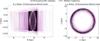 |
Fig. 1 Monte Carlo ensemble of 1I/’Oumuamua trajectories in the R - z plane. The transparent lines show 50 representative orbits from the uncertainty distribution, and the median trajectory is shown as a thick solid curve suitable for black-and-white printing. |
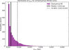 |
Fig. 2 Distribution of maximum vertical excursions zmax for 1I/’Oumuamua from our Monte Carlo analysis. The vertical lines indicate the median and the 16th and 84th percentiles. |
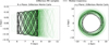 |
Fig. 3 Monte Carlo ensemble of 2I/Borisov trajectories in the R - z plane. The transparent lines show 50 representative orbits from the uncertainty distribution, and the median trajectory is shown as a thick solid curve suitable for black-and-white printing. |
2.3 2I/Borisov
The Monte Carlo trajectories of 2I/Borisov in the R-z plane are shown in Fig. 3, and the resulting zmax distribution is presented in Fig. 4. The ensemble analysis yielded a median maximum vertical excursion of zmax = 0.121 kpc. The 16th-84th percentile interval was 0.111-0.131 kpc, while the full Monte Carlo sample spanned 0.085-0.171 kpc. This intermediate zmax value places 2I/Borisov in a regime consistent with moderately heated thin-disk stars, indicating that the comet’s vertical excursions are comparable to solar-type orbits.
2.4 3I/ATLAS
Figure 5 displays the Monte Carlo R-z trajectories for 3I/ATLAS, while Fig. 6 shows the corresponding distribution of maximum vertical excursions zmax. The ensemble analysis yielded a median maximum vertical excursion of zmax = 0.481 kpc. The 16th-84th percentile interval was 0.464-0.504 kpc, while the full Monte Carlo sample spanned 0.422-0.630 kpc. This high zmax value, approaching half a kiloparsec, exceeds the scale heights of young thin-disk stars and solar-age populations. It is comparable to thick-disk vertical excursions and is therefore consistent with an older disk population under our adopted kinematic model.
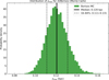 |
Fig. 4 Distribution of maximum vertical excursions zmax for 2I/Borisov from our Monte Carlo analysis. The vertical lines indicate the median and the 16th and 84th percentiles. |
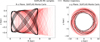 |
Fig. 5 Monte Carlo ensemble of 3I/ATLAS trajectories in the R - z plane. The transparent lines show 50 representative orbits from the uncertainty distribution, and the median trajectory is shown as a thick solid curve suitable for black-and-white printing. |
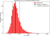 |
Fig. 6 Distribution of maximum vertical excursions zmax for 3I/ATLAS from our Monte Carlo analysis. The vertical lines indicate the median and the 16th and 84th percentiles. |
3 Probability distribution of age
Next, we evaluate the probability distribution p(t) (with unit normalization ∫p(t) dt = 1) for the age t of the interstellar objects. This inference is conditioned on the hypothesis that the ISOs were produced by stellar populations in the Galactic disk and therefore sample the same underlying age distribution as those stars. We base our analysis on the extent of their vertical excursions, quantified by the maximum vertical value zmax reached by their orbits, given that the disk scale height increases with stellar age. Possible nonstellar production channels (e.g., ejection from giant molecular cloud environments or clustered star-forming regions) are acknowledged but not modeled here.
3.1 Bayesian statistical framework
We implemented a Bayesian statistical framework that combines the Monte Carlo orbital results with theoretical models of stellar kinematics. The likelihood was computed numerically by drawing vertical velocities, mapping them to turning points in the adopted vertical potential, and evaluating the empirical distribution of zmax. For the prior, we used a digitized and tabulated approximation to the Milky Way star formation history inferred by Fantin et al. (2019), normalized over the age support (013.5 Gyr). We also report sensitivity to alternative priors in Appendix A.
3.1.1 Theoretical foundation
The Bayesian approach relies on the correlation between stellar age and vertical velocity dispersion in the Galactic disk. Young stellar populations exhibit smaller dispersions, while older populations show larger dispersions after long-term dynamical heating.
Our posterior probability for stellar age τ given observed maximum vertical height zmax follows Bayes’ theorem:
 (1)
(1)
where P(zmax|τ) is the likelihood function and SFR(τ) represents the star formation rate prior encoding when stars formed in Galactic history.
3.1.2 Likelihood
We compute P(zmax|τ) from the vertical turning point condition in the adopted potential,
 (2)
(2)
so that ΔΦ(zmax) ≡ Φ(zmax) — Φ(0) =  . Let zturn(v) ≥ 0 denote the nonnegative solution of ΔΦ(z) =
  . The induced likelihood is
![Mathematical equation: P(z_{\text{max}}|\tau) = \int_{-\infty}^{\infty} \mathcal{N}(v_z;0,\sigma_W^2(\tau))\,\delta\!\left[z_{\text{max}} - z_{\text{turn}}(|v_z|)\right]\,{\rm d}v_z,](/articles/aa/full_html/2026/05/aa56405-25/aa56405-25-eq6.png) (3)
(3)
which we evaluate using Monte Carlo draws of vz, solving for zmax in the adopted potential, and a kernel density estimate (KDE) of the resulting zmax samples. We enforce the physical boundary zmax ≥ 0 by reflecting the KDE samples about zero, which removes bias near zmax = 0.
3.1.3 Numerical implementation and convergence
The likelihood was evaluated on an age grid spanning 0-13.5 Gyr at 1 Myr resolution and used a cubic interpolant for the prior. At each age we drew Nvz = 600 velocities from N(0, σW(τ)) with a fixed random seed and computed turning points in the adopted vertical potential. We estimated P(zmax|τ) via KDE on the resulting zmax samples. We verified stability by comparing 1 Myr versus 10 Myr grids and by extending the upper bound to 16 Gyr; posterior summaries are unchanged at the quoted precision.
3.1.4 Age-dependent velocity dispersion
We adopted a velocity dispersion model σW(τ) that captures thin and thick disk trends with a smooth transition. The thin disk component follows a power law reflecting gradual dynamical heating:
 (4)
(4)
with σ1 = 8.0 km s−1 and β = 0.5. The thick disk component uses a constant plateau σthick = 40.0 km s−1 .To avoid an unphysical discontinuity, we blended these components smoothly via a tanh function:
![Mathematical equation: f(\tau) &=& \frac{1}{2}\left[1 + \tanh\left(\frac{\tau - \tau_{\rm thick}}{\Delta\tau}\right)\right],\\](/articles/aa/full_html/2026/05/aa56405-25/aa56405-25-eq8.png) (5)
(5)
 (6)
(6)
where τthick = 7.0 Gyr marks the thin-thick transition and Δτ = 0.5 Gyr controls the transition width. This smooth formulation avoids numerical artifacts while preserving the kinematic dichotomy; in the limit Δτ → 0, it recovers a sharp piecewise model.
The power-law component reflects gradual dynamical heating from gravitational scattering by giant molecular clouds and other perturbers (e.g., Kokubo & Ida 1992; Aumer & Binney 2009). With these parameters, σW(10 Gyr) ≈ 40 km s−1, consistent with thick-disk kinematics. The transition at 7 Gyr reflects the observed kinematic dichotomy in Galactic stellar populations, where stars older than this age exhibit systematically higher velocity dispersions, motivated by LAMOST-Gaia observations (Yu & Liu 2018). We explored 35-45 km s−1 plateaus and steeper exponents in sensitivity tests; in all cases, the resulting posterior median ages change by less than the reported credible intervals.
3.1.5 Star-formation-rate prior
We took a digitized and tabulated approximation to the Fantin et al. (2019) star formation history and defined the prior by normalization:
, \qquad 0 \le \tau \le 13.5~\mathrm{Gyr},\\](/articles/aa/full_html/2026/05/aa56405-25/aa56405-25-eq10.png) (7)
(7)
 (8)
(8)
Here Icub denotes a cubic interpolant of the digitized Fantin curve, and we set SFRFantin(τ) = 0 outside the support. We truncated negative interpolated values to zero before renormalizing on the same support. We assessed prior sensitivity by comparing against an exponential form and a flat prior (see Appendix A).
3.2 Bayesian age inference results
The posterior age distributions for lI/’Oumuamua, 2I/Borisov, and 3I/ATLAS are shown in Figs. 7, 8, and 9, respectively, and are compared in Fig. 10. The Bayesian analysis yields age estimates that follow the expected trend with zmax:
1I/’Oumuamua (young stellar system): median age of 3.2 Gyr with a 68% credible interval (CI) of 0.5-8.8 Gyr. The zmax value is consistent with a young origin, although the posterior retains a tail to older ages.
2I/Borisov (intermediate-age population): median age of 5.0 Gyr with a 68% credible interval of 1.8-9.7 Gyr. The moderate zmax indicates origin from thin disk stars with intermediate levels of dynamical heating.
3I/ATLAS (older disk with thick-disk-like kinematics): median age of 8.7 Gyr with a 68% credible interval of 5.2-10.3 Gyr. The high zmax value requires high velocity dispersions characteristic of ancient thick disk populations.
These classifications depend on the adopted age-velocitydispersion relation and disk-heating model.
Our posteriors reflect two drivers: (i) the measured zmax, which sets the likelihood’s support across age and (ii) the star formation prior, which upweights epochs with higher stellar birth rates. For 1I and 2I, moderate zmax values favor thin-disk ages with broad tails; for 3I, the high zmax value shifts probability to older, thick-disk times. The widths of the credible intervals mainly trace measurement covariances in the inbound state and reasonable variations in σW(τ).
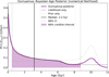 |
Fig. 7 Posterior age distribution for 1I/’Oumuamua. The median age is 3.2 Gyr with a 68% CI [0.5, 8.8] Gyr. |
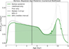 |
Fig. 8 Posterior age distribution for 2I/Borisov. The median age is 5.0 Gyr with a 68% CI [1.8, 9.7] Gyr. |
 |
Fig. 9 Posterior age distribution for 3I/ATLAS. The median age is 8.7 Gyr with a 68% CI [5.2, 10.3] Gyr. |
4 Discussion
Our Bayesian age inference results can be compared directly with previous investigations of interstellar object origins and ages, thereby providing context for our findings and clarifying methodological differences. For 1I/’Oumuamua, Almeida-Fernandes & Rocha-Pinto (2018) inferred ages <2 Gyr from kinematic arguments, broadly consistent with our median of 3.2 Gyr (68% CI: 0.5-8.8 Gyr). Hallatt & Wiegert (2020) argued for very young origins based on low velocity dispersions relative to the LSR; our credible interval does not include ages <100 Myr. Hsieh et al. (2021) linked 1I/’Oumuamua to nearby young associations (∼30 Myr) via backtracking; differences relative to our results stem from methodology (association matching versus probabilistic kinematics). See also Gaidos, Williams & Kraus (2017) for an early young-association hypothesis. For 2I/Borisov, initial characterization showed typical cometary properties (Guzik et al. 2020). For 3I/ATLAS, Taylor & Seligman (2025) reported a kinematic age range of ∼3-11 Gyr under an equivalence assumption between ISO and stellar age-velocity relations; our median of 8.7 Gyr (68% CI: 5.210.3 Gyr) aligns with the older end of their interval. Recently, Hopkins et al. (2025) presented a related analysis of ISO kinematics and likewise found that 3I/ATLAS is consistent with an old disk population. Our results differ from Almeida-Fernandes & Rocha-Pinto (2018) primarily because they used the full 3D Galactocentric velocity, whereas we conditioned on the maximum vertical excursion zmax.
Trajectory-based searches for stellar origins emphasize the difficulty of precise backtracking over long timescales owing to dynamical heating and measurement uncertainties (e.g., Bailer-Jones et al. 2018). Our approach complements these efforts by focusing on demographic age inference rather than on identifying specific progenitors. For priors on formation history, our baseline is a smooth interpolation to Fantin et al. (2019), with sensitivity to alternative priors shown in Appendix A.
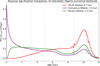 |
Fig. 10 Comparison of Bayesian age posteriors for all three interstellar objects. 1I/’Oumuamua (purple), 2I/Borisov (green), and 3I/ATLAS (red) show distinct median ages. |
5 Conclusions
We developed a framework for constraining the origins of interstellar objects through Galactic orbital analysis and Bayesian age inference. Our approach complements prior kinematic age inferences by focusing on zmax-conditioned posteriors rather than full 3D velocities.
We performed ensemble calculations using 10000 orbital realizations per object to account for measurement uncertainties in both interstellar object velocities and solar motion parameters. This approach yielded statistical distributions of maximum vertical excursions: zmax = 0.016 ± 0.002 kpc for 1I/’Oumuamua, 0.121 ± 0.010 kpc for 2I/Borisov, and  kpc for 3I/ATLAS.
We implemented a statistical framework that combines the orbital zmax measurements with models of stellar kinematics. The methodology uses a numerical likelihood (with no closed form) and an age-dependent velocity dispersion that captures observed thin-thick disk trends. Our analysis yields quantitative age estimates: 1I/’Oumuamua is consistent with a young stellar system (3.2 Gyr, 68% CI: 0.5-8.8 Gyr), 2I/Borisov with an intermediate-age population (5.0 Gyr, 68% CI: 1.8-9.7 Gyr), and 3I/ATLAS with an older disk population (8.7 Gyr, 68% CI: 5.2-10.3 Gyr).
The results demonstrate the expected age trend in which smaller vertical excursions correspond to younger stellar origins. 1I/’Oumuamua's confined orbit is consistent with ejection from a relatively young stellar system in the thin Galactic disk. 2I/Borisov's moderate excursions suggest an origin in a solar-age thin-disk population. 3I/ATLAS's large vertical range is consistent with velocity dispersions characteristic of older disk populations. We refrain from attributing specific formation mechanisms for thick-disk stars, given ongoing debates. Our Bayesian framework links the orbital zmax measurements to simple disk-heating models, providing a practical way to report age estimates with credible intervals. Over many orbital times, the trajectories are expected to migrate radially as a result of transient features such as spiral arms or the Galactic bar (Sellwood & Binney 2002). These constraints apply under the assumption that ISOs and disk stars have experienced comparable vertical heating in the Galactic potential; deviations from this assumption would shift the inferred ages. Excess ejection speeds relative to parent stars can shift the inferred ages in either direction; we did not explicitly model ejection-speed distributions here. We also refrain from inferring specific formation pathways from the current sample; the distinct median ages are consistent with multiple possible origins, but more objects will be required to draw firm demographic conclusions.
Data availability
Supplementary material supporting this article is available at Zenodo: https://sandbox.zenodo.org/records/473317
Acknowledgements
We thank Matthew Hopkins for his careful cross-checking of our paper. This work was supported in part by Harvard University, the Black Hole Initiative and the Galileo Project.
References
- Almeida-Fernandes, F., & Rocha-Pinto H. J. 2018, MNRAS, 480, 4903 [Google Scholar]
- Aumer, M., Binney, J. J. 2009, MNRAS, 397, 1286 [NASA ADS] [CrossRef] [Google Scholar]
- Bailer-Jones, C. A. L., Farnocchia, D., Meech, K. J., Brasser, R., Micheli, M., Chakrabarti, S., Buie, M. W., et al. 2018, AJ, 156, 205 [Google Scholar]
- Bailer-Jones, C. A. L., Farnocchia, D., Ye, Q., Meech, K. J., Micheli, M. 2020, A&A, 634, A14 [NASA ADS] [CrossRef] [EDP Sciences] [Google Scholar]
- Sellwood, J. A., Binney, J. J. 2002, MNRAS, 336, 785 [NASA ADS] [CrossRef] [Google Scholar]
- Fantin, N. J., Côté, P., McConnachie, A. W., et al. 2019, ApJ, 887, 148 [NASA ADS] [CrossRef] [Google Scholar]
- Hallatt, T., Wiegert, P. 2020, AJ, 159, 147 [Google Scholar]
- Hsieh, C.-H., Laughlin, G., Arce, H. G. 2021, ApJ, 917, 20 [NASA ADS] [CrossRef] [Google Scholar]
- Jewitt, D. 2024, Handbook of Exoplanets, Interstellar Objects in the Solar System (Berlin: Springer) [Google Scholar]
- Jewitt, D., & Seligman, D. Z. 2023, Ann. Rev. Astron. Astrophys., 61, 197 [Google Scholar]
- Kokubo, E., Ida, S. 1992, PASJ, 44, 601 [Google Scholar]
- Loeb, A., MacLeod, M. 2024, A&A, 686, A123 [NASA ADS] [CrossRef] [EDP Sciences] [Google Scholar]
- Mamajek, E. 2017, Res. Notes Am. Astron. Soc., 1, 21 [Google Scholar]
- Meech, K. J., Weryk, R., Micheli, M., et al. 2017, Nature, 552, 378 [Google Scholar]
- McMillan, P. J. 2017, MNRAS, 465, 76 [NASA ADS] [CrossRef] [Google Scholar]
- Põder, S., Benito, M., Pata, J., et al. 2023, A&A, 676, A134 [NASA ADS] [CrossRef] [EDP Sciences] [Google Scholar]
- Robin, A. C., Bienaymé, O., Salomon, J. B., et al. 2022, A&A, 667, A98 [NASA ADS] [CrossRef] [EDP Sciences] [Google Scholar]
- Siraj, A., Loeb, A. 2022a, AsBio, 22, 1459 [Google Scholar]
- Siraj, A., Loeb, A. 2022b, ApJ, 939, 53 [NASA ADS] [CrossRef] [Google Scholar]
- Williams, G. V. 2017, Minor Planet Electronic Circulars, 2017-V17 [Google Scholar]
- Yu, J., Liu, C. 2018, MNRAS, 475, 1093 [Google Scholar]
- Zhang, Y., Lin, D. N. C. 2020, NatAs, 4, 852 [Google Scholar]
- Hopkins, M. J., Dorsey, R. C., Forbes, J. C., et al. 2025, ApJ, 990, L30 [Google Scholar]
- Seligman, D. Z., Micheli, M., Farnocchia, D., et al. 2025, ApJ, 989, L36 [Google Scholar]
- Taylor, A. G., & Seligman, D. Z. 2025, ApJ, 990, L14 [Google Scholar]
- Gaidos, E., Williams, J., Kraus, A. 2017, RNAAS, 1, 13 [Google Scholar]
- Guzik, P., Drahus, M., Rusek, K., Waniak, W., et al. 2020, NatAs, 4, 53 [Google Scholar]
Appendix A Diagnostics and sensitivity tests
This appendix provides supporting diagnostics for the Bayesian age inference described in Sect. 3, specifically the sensitivity of the posteriors to alternative star formation priors. The figures below (Figs. A.1-A.3) summarize these tests for each object.
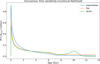 |
Fig. A.1 Prior sensitivity for 1I/’Oumuamua. The posterior is recomputed using the Fantin prior, a flat prior, and an exponential prior. |
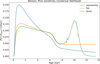 |
Fig. A.2 Prior sensitivity for 2I/Borisov. The posterior is recomputed using the Fantin prior, a flat prior, and an exponential prior. |
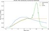 |
Fig. A.3 Prior sensitivity for 3I/ATLAS. The posterior is recomputed using the Fantin prior, a flat prior, and an exponential prior. |
All Figures
|
Fig. 1 Monte Carlo ensemble of 1I/’Oumuamua trajectories in the R - z plane. The transparent lines show 50 representative orbits from the uncertainty distribution, and the median trajectory is shown as a thick solid curve suitable for black-and-white printing. |
| In the text | |
|
Fig. 2 Distribution of maximum vertical excursions zmax for 1I/’Oumuamua from our Monte Carlo analysis. The vertical lines indicate the median and the 16th and 84th percentiles. |
| In the text | |
|
Fig. 3 Monte Carlo ensemble of 2I/Borisov trajectories in the R - z plane. The transparent lines show 50 representative orbits from the uncertainty distribution, and the median trajectory is shown as a thick solid curve suitable for black-and-white printing. |
| In the text | |
|
Fig. 4 Distribution of maximum vertical excursions zmax for 2I/Borisov from our Monte Carlo analysis. The vertical lines indicate the median and the 16th and 84th percentiles. |
| In the text | |
|
Fig. 5 Monte Carlo ensemble of 3I/ATLAS trajectories in the R - z plane. The transparent lines show 50 representative orbits from the uncertainty distribution, and the median trajectory is shown as a thick solid curve suitable for black-and-white printing. |
| In the text | |
|
Fig. 6 Distribution of maximum vertical excursions zmax for 3I/ATLAS from our Monte Carlo analysis. The vertical lines indicate the median and the 16th and 84th percentiles. |
| In the text | |
|
Fig. 7 Posterior age distribution for 1I/’Oumuamua. The median age is 3.2 Gyr with a 68% CI [0.5, 8.8] Gyr. |
| In the text | |
|
Fig. 8 Posterior age distribution for 2I/Borisov. The median age is 5.0 Gyr with a 68% CI [1.8, 9.7] Gyr. |
| In the text | |
|
Fig. 9 Posterior age distribution for 3I/ATLAS. The median age is 8.7 Gyr with a 68% CI [5.2, 10.3] Gyr. |
| In the text | |
|
Fig. 10 Comparison of Bayesian age posteriors for all three interstellar objects. 1I/’Oumuamua (purple), 2I/Borisov (green), and 3I/ATLAS (red) show distinct median ages. |
| In the text | |
|
Fig. A.1 Prior sensitivity for 1I/’Oumuamua. The posterior is recomputed using the Fantin prior, a flat prior, and an exponential prior. |
| In the text | |
|
Fig. A.2 Prior sensitivity for 2I/Borisov. The posterior is recomputed using the Fantin prior, a flat prior, and an exponential prior. |
| In the text | |
|
Fig. A.3 Prior sensitivity for 3I/ATLAS. The posterior is recomputed using the Fantin prior, a flat prior, and an exponential prior. |
| In the text | |
Current usage metrics show cumulative count of Article Views (full-text article views including HTML views, PDF and ePub downloads, according to the available data) and Abstracts Views on Vision4Press platform.
Data correspond to usage on the plateform after 2015. The current usage metrics is available 48-96 hours after online publication and is updated daily on week days.
Initial download of the metrics may take a while.