© The Authors 2026

1 Introduction

In Roupas (2025) (hereafter Paper I) we proposed a channel for the black hole (BH) mass growth via gas accretion in proto-stellar clusters to values within the upper BH mass gap, induced by the physics of a pair-instability supernova (PISN) (Belczynski et al. 2016; Spera & Mapelli 2017; Woosley & Heger 2021), 60 M_⊙ ≲ m_BH ≲ 130 M_⊙, and up to the intermediate-massive-black-hole (IMBH) regime of m_BH ~ 10³ M_⊙. Gas-rich, compact, low-metallicity, massive stellar clusters provide ideal conditions for the mass growth of stellar BHs via accretion. Mass segregation, which drives the massive stellar progenitors of BHs toward the dense center of the cluster (Spitzer 1987), is accelerated in the presence of ambient gas remaining from the first stellar formation event, at timescales of ≲1 Myr (Leigh et al. 2014). Moreover, in a lower-metallicity environment stellar winds get weaker, allowing for longer gas-depletion timescales in the cluster, despite PISN feedback, for sufficiently compact clusters (Paper I).

Recent observations by the James Webb Space Telescope (JWST) revealed five proto-stellar cluster candidates in the Cosmic Gems arc galaxy at high redshift, z = 10.2, (Adamo et al. 2024), which present low metallicity and are remarkably compact. Their typical masses are ~10⁶ M_⊙ and half-light radii ~1 pc. Such proto-stellar clusters are plausibly the progenitors of globular clusters (GCs) (Kruijssen 2015; Renzini 2017; Elmegreen 2018). These JWST observations provide observationally motivated cluster parameters for our models.

The semi-analytic framework of stellar-BH growth in such environments, introduced in Paper I, incorporates gas depletion by stellar feedback, distinct BH formation times depending on stellar progenitors and formation channel, dynamical friction, stochastic stellar encounters, turbulence, and gas accretion. Here we extend this model to include the BH spin evolution. This calculation is essential for identifying our proposed channel regarding the astrophysical origin of gravitational-wave (GW) signals, among different stellar-BH mass growth channels. These include the repeated BH merger channel (Miller & Hamilton 2002; O’Leary et al. 2006; Gerosa & Berti 2017), and gas accretion in active galactic nucleus (AGN) disks (Levin 2007; McKernan et al. 2012; Yi et al. 2018; Yang et al. 2020) as well as in the cores of proto-galactic haloes (Safarzadeh & Haiman 2020; Bartos & Haiman 2025).

Identifying the origin of heavy BHs ~ 10²–10³ M_⊙ is a timely, active area of research (Gerosa & Berti 2017; Roupas & Kazanas 2019; Baibhav et al. 2020; Renzo et al. 2020; Kimball et al. 2020; Safarzadeh & Haiman 2020; Mapelli et al. 2021; Rizzuto et al. 2022; Arca Sedda et al. 2023; Torniamenti et al. 2024; Fujii et al. 2024; Purohit et al. 2024; Baumgarte & Shapiro 2025; Lee et al. 2025; Bartos & Haiman 2025; Kıroğlu et al. 2025; Gottlieb et al. 2025; Liu et al. 2025). The GW experiments, LIGO-Virgo-KAGRA Collaborations, have revealed a significant population of BHs within the upper BH mass gap (Abbott et al. 2023). The most recent such GW signal, GW231123 (Abac et al. 2025), involves components that are heavy, ${103}_{-52}^{+20}$ M_⊙, ${137}_{-17}^{+22}$ M_⊙, and that have high spins, ${0.9}_{-0.19}^{+0.10}$, ${0.8}_{-0.51}^{+0.20}$. These values are difficult to explain within the repeated-merger scenario, which predicts a narrow peak at ~0.7 (Fishbach et al. 2017). We show here that these mass and spin values naturally emerge via accretion in gas-rich proto-stellar clusters.

The BH motion is repeatedly deflected by stochastic gravitational perturbations – two-body encounters and turbulent gas motions – that reorient the BH trajectory. Angular-momentum inflow is induced by the velocity shear within the BH’s sphere of influence, which can produce an accretion disk. These successive episodes lead to an accretion regime, where a broad range of spin values, ~0–0.97, is possible, with a strong spin-mass correlation, as we demonstrate below.

In the next section we review the cluster and BH motion model of Paper I. In Sect. 3 we describe the BH spin evolution and accretion disk models. Section 4 presents our results, and we conclude in Sect. 5.

2 Cluster physical model

We adopted the same semi-analytic model as we introduced in Paper I for the proto-stellar cluster and the BH motion. We briefly summarize the main elements in this section and refer the reader to Paper I for further details.

2.1 Gas depletion timescale

In gaseous proto-stellar clusters, stellar winds and supernova (SN) explosions inject energy into the ambient gas, driving gas depletion. Theoretical arguments and observational evidence indicate that the depletion timescale depends primarily on the compactness of the cluster (Krause et al. 2016; Roupas 2025), $$C\equiv \frac{M/{10}^5{\mathrm{M}}_{\odot }}{r_{\mathrm{h}}},$$(1)

rather than on the cluster mass alone. A simple theoretical understanding follows from noting that the binding energy scales as U ∝ M²/R ~ C · M, and therefore increases linearly with the total mass for a fixed initial compactness, while the total stellar feedback energy scales as E_feed ∝ M regardless of compactness. Consequently, compactness – not mass – primarily determines the relative energy balance between feedback and gravitational binding. The star formation efficiency is also crucial in setting the depletion timescale, as it regulates both the available gas reservoir and the total energy released by stellar feedback. A third key parameter is metallicity, which influences stellar wind luminosities and stellar lifetimes, and thereby the onset of SN feedback. In this work we focus on low-metallicity clusters (Z ~ 0.01 Z_⊙) motivated by high-redshift JWST observations of the Cosmic Gems arc galaxy.

In Fig. 1, we display the depletion timescale, τ, as a function of compactness for several values of ε. This calculation is based on our detailed model presented in Paper I, where corresponding figures for solar and sub-solar metallicities are also provided. In our model τ is defined as the time when the cumulative energy from stellar winds and SN equals the binding energy. We took into account the stellar lifetimes dependence on stellar masses, extrapolating the tabulated data, referring to low-metallicity stars, of Groh et al. (2019). Stellar-wind and SN energy injection was modeled based on a careful consideration of observations and numerical data (Vink et al. 2001; Kudritzki 2002; Puls et al. 2008; Krause et al. 2013; Renzo et al. 2017; Sander & Vink 2020). We observe in Fig. 1a characteristic stall at $${\tau }_{\text{stall\hspace{0.17em}}}\approx 2.9\mathrm{M}\mathrm{y}\mathrm{r}$$(2)

that marks the onset of PISNe for the adopted parameters. The range of compactness values for the observed proto-stellar clusters in the Cosmic Gems arc galaxy – the same range as is used in our simulations – corresponds to this stall timescale.

Fig. 1 Depletion timescale, τ, with respect to the compactness, C, of a gaseous stellar cluster of any total mass at low metallicity (~0.01Z⊙) for different possible star formation efficiencies, ε.

2.2 Black hole motion

In order to simulate the motion of BHs, we implemented the same model as in Paper I, briefly summarized as follows. We assumed background gas and stellar Plummer density profiles, taking into account the expansion of the cluster due to the mass loss, the higher extension of the gas component relative to the stellar one, the gas temperature profile, and the gas cooling over time. We adopted an exponential law of gas depletion (Baumgardt & Kroupa 2007), $${\dot{M}}_{\mathrm{g}\mathrm{a}\mathrm{s}}=-\frac{M_{\mathrm{g}\mathrm{a}\mathrm{s}}}{\tau },$$(3)

since the stellar feedback processes, responsible for gas depletion, generate energy proportional to the cluster mass. We terminated each run once 99% of the initial gas mass had been depleted. In practice, the BH mass and spin evolution stalled even earlier, when ~95% of the gas had been removed.

At each simulation run, we generated a BH population from a Salpeter BH initial mass function (Perna et al. 2019) sampling positions and velocities from the Brownian probability density of Roupas (2021). Each BH was created at a different time depending on the zero-age main sequence (ZAMS) progenitor mass. We classified the BHs into several types depending on the ZAMS progenitor mass assumed to drive the related formation channel: a core-collapse-SN (CCSN), direct collapse of low or high ZAMS mass, and pulsational-pair-instability-SN (PPISN) of low or high ZAMS mass. We applied a recoil kick at birth to the BH remnants of CCSN that injected ~70% of such BHs out of the cluster.

We evolved all BHs in the evolving background gas and stellar profiles, integrating the BHs equations of motion with a standard drift-kick scheme. The deterministic forces – gravity and dynamical friction from the background – were implemented using an adaptive Runge-Kutta method, while stochastic velocity increments due to both stellar perturbations and gas turbulencewe were applied at adaptive timesteps, Δt_stoch, as is described in detail in Paper I. The local gravitational dynamical timescale, ${\tau }_{\text{grav}}(r_{•})=\sqrt{r_{•}^3/(G{M}_{\text{enc}}(r_{•}))}\sim 1/\sqrt{G⟨{\rho }_{\text{tot}}(r_{•})⟩}$, is the typical orbital timescale of the local perturber population. It is therefore a natural choice for setting the reference scale of the timestep, Δt_stoch, for applying stochastic kicks. We further imposed consistency bounds, which are discussed in detail in Appendix A. In Fig. 2 we plot the contour of the median $\tilde{\mathrm{\Delta }}{t}_{\text{stoch}}$ with respect to the median BH position and the final BH mass for an indicative run of our typical cluster. It is $\tilde{\mathrm{\Delta }}{t}_{\text{stoch}}=\mathcal{O}({10}^{-2}\mathrm{M}\mathrm{y}\mathrm{r})$ and can become as low as ~0.007 Myr for more heavy BHs, m_•,f ≳ 50 M_⊙, which move on average deeper in the cluster core.

We adopted an isotropic hot-type accretion, whose typical representative is Bondi-Hoyle accretion (Merritt 2013) given the dense, hot, turbulent gaseous environment. The spherically symmetric accretion rate is (Frank et al. 2002) $${\dot{m}}_{\mathrm{f}\mathrm{e}\mathrm{e}\mathrm{d}}=\pi {\rho }_{\mathrm{g}\mathrm{a}\mathrm{s}}{v}_{\mathrm{r}\mathrm{e}\mathrm{l}}{R}_{\mathrm{a}\mathrm{c}\mathrm{c}}^2,v_{\mathrm{r}\mathrm{e}\mathrm{l}}=\sqrt{v_{•}^2+c_s^2}.$$(4)

The appropriate value of the accretion radius, R_acc, depends on the relative amount of gas and the radial position of the accretor (Bonnell et al. 2001). If the gas dominates the cluster potential at a certain BH position, r_•, the accretion rate is determined by a tidal-lobe accretion radius (Paczyński 1971), $$R_{\mathrm{t}\mathrm{i}\mathrm{d}}\left(r_{•}\right)\sim 0.5{\left(\frac{m_{\mathrm{B}\mathrm{H}}}{M(r<r_{•})}\right)}^{1/3}{r}_{•},$$(5)

where M(r < r_•) is the total mass of the cluster within the BH radial position. Otherwise, when gas is less dominant, the appropriate accretion radius is the Bondi-Hoyle radius, R_B: $$R_{\mathrm{B}}=\frac{2G{m}_{\mathrm{B}\mathrm{H}}}{v_{\mathrm{r}\mathrm{e}\mathrm{l}}^2}.$$(6)

We assumed the accretion radius to be the smaller of the two at any instant in time (Bonnell et al. 2001), $$R_{\mathrm{a}\mathrm{c}\mathrm{c}}(t)=min\{R_{\mathrm{B}}(t),R_{\mathrm{t}\mathrm{i}\mathrm{d}}(t)\},$$(7)

adopting the most conservative assumption. Furthermore, we adopted a maximum threshold for the accretion rate of $${\dot{m}}_{\mathrm{a}\mathrm{c}\mathrm{c}}(t)=min\{{\dot{m}}_{\mathrm{f}\mathrm{e}\mathrm{e}\mathrm{d}}(t),10{\dot{m}}_{\mathrm{E}\mathrm{d}\mathrm{d},0}\},$$(8)

where ${\dot{m}}_{\mathrm{E}\mathrm{d}\mathrm{d},0}=4\pi G{m}_{\mathrm{B}\mathrm{H}}{m}_p/{\eta }_0{\sigma }_{T}c$ is the reference Eddington rate value for the radiative efficiency, η₀ = 0.057. This is based on the results of Inayoshi et al. (2016), who showed that for $1<{\dot{m}}_{\text{feed}}/{\dot{m}}_{\text{Edd},0}<100$ the mean accretion rate cannot exceed $⟨{\dot{m}}_{\text{acc}}⟩\lesssim 10{\dot{m}}_{\text{Edd},0}$. We adopted this constant cap as a simple, conservative assumption, since Inayoshi et al. (2016) reported that there occur episodic bursts of accretion rate comparable to ${\dot{m}}_{\text{feed}}$ that violate the general cap for the mean rate. In practice, in the physical conditions we consider here and for m_BH ≲ 10³ M_⊙ we have $0<{\dot{m}}_{\text{feed}}(t)/{\dot{m}}_{\text{Edd},0}<10$, automatically satisfying the cap.

Fig. 2 Contour of the median stochastic timestep, $\tilde{\mathrm{\Delta }}{t}_{\text{stoch}}$, with respect to the median BH position, ${\tilde{r}}_{\mathrm{B}\mathrm{H}}$, and the final BH mass, mBH,f, for an indicative run of our typical cluster, M⋆ = 106 M⊙, rc,⋆ = 1 pc ε = 0.35.

3 BH-spin evolution and accretion disk

Our primary goal is to quantify the possible spin-up of stellar BHs through accretion in proto-stellar clusters. A stellar BH is formed with low spin from its progenitor star if there is efficient angular-momentum transfer. The magnetic Tayler instability may efficiently couple the stellar core to its envelope (Spruit 2002), enabling angular momentum to be transported outward during core contraction and thereby preventing the core from spinning up. Simulations indicate that the BH formed at collapse is expected to have a very low natal spin, with a typical value of a_* ≃ 0.01 (Fuller & Ma 2019), where the dimensionless spin is $a_{\ast }\equiv J_{\mathrm{B}\mathrm{H}}c/(G{m}_{\mathrm{B}\mathrm{H}}^2)$ and J_BH the BH spin. We adopted this value for the initial BH spin magnitudes.

Regarding the initial BH spin orientations, we assumed an isotropic distribution inherited from an isotropic distribution of stellar spin axes. This assumption is consistent with observational analyses (Jackson & Jeffries 2010; Healy et al. 2023). It is also intuitively justified, at least for nonrotating clusters, by the turbulent nature of star-forming environments. We note, nevertheless, that rotating clusters with sufficient rotational energy may induce partially stellar spin alignment (Corsaro et al. 2017). We do not consider this case here.

3.1 Disk formation

The BH motion is repeatedly perturbed at stochastic timesteps, as is discussed in Appendix A. The acquired BH azimuthal velocity induces apparent transverse velocity gradients within the accretion sphere (|r − r_•| ≤ R_acc) as the sphere gets advected along the BH trajectory. Numerical simulations of angular-momentum accretion, driven by velocity and density gradients, show the formation of an accretion disk (Ruffert & Anzer 1995). More recently, Tripathi et al. (2025) demonstrated that an off-axis (“lateral”) Bondi-Hoyle-Lyttleton flow, characterized by an antisymmetric transverse velocity field, naturally generates angular momentum and produces a persistent disk.

In our system the transverse velocity gradient is generated within the accretion radius by the BH azimuthal velocity, gained after a perturbation event, with |Δv_⊥| ≈ 2|ω_BH|R_acc (perpendicular to the position vector r_•) on the induced orbital plane, where $${\omega }_{\mathrm{B}\mathrm{H}}=\frac{1}{r_{•}^2}{r}_{•}\times v_{•}.$$(9)

The velocity shear across R_acc produces a net angular momentum as the apparent gas transverse velocity in the BH rest frame differs between the inner (proximate to the cluster center) and outer hemispheres, creating a shear flow opposite to the BH’s orbital motion. This asymmetric inflow provides angularmomentum injection within the BH’s accretion radius R_acc. At the BH orbital plane, this shear specific angular momentum of the gas is $j_0\approx -2{\omega }_{\mathrm{B}\mathrm{H}}{R}_{\mathrm{a}\mathrm{c}\mathrm{c}}^2$. Volume-averaging over all planes within R_acc (using R_plane = R_acc cos θ, θ measured from the orbital plane) and weighting by the volume element ∝ cos² θ, we obtain the geometric prefactor: $2{\int }_{-\pi /2}^{\pi /2}{\cos }^4\theta \mathrm{d}\theta /{\int }_{-\pi /2}^{\pi /2}{\cos }^2\theta \mathrm{d}\theta =3/2$. Thus, we get the total specific shear angular momentum injected into the accretion radius, $$j\approx -\frac{3}{2}{\omega }_{\mathrm{B}\mathrm{H}}{R}_{\mathrm{a}\mathrm{c}\mathrm{c}}^2,$$(10)

where the minus sign indicates that the shear generates retrograde inflow relative to BH orbital motion. The accretion radius is defined in Eq. (7). Both the orientation and approximate magnitude of our estimate, Eq. (10), is consistent with numerical simulations of angular-momentum accretion driven by velocity gradients (Ruffert & Anzer 1995; Tripathi et al. 2025).

Note that all BH-dependent quantities are local and time-dependent, such as j = j(r_•, t), although we omit this dependence to simplify our notation. There is also an angular momentum component (j_grad) induced by the density gradient within R_acc. For the smooth cluster density profiles in our models, this is negligible because ${\mathit{j}}_{\text{grad}}\approx \left(\mathrm{\Delta }{m}_{\text{in}-\text{out}}/m_{\text{acc}}\right){\omega }_{\text{BH}}{R}_{\text{acc\hspace{0.17em}}}^2$ with Δm_in–out/m_acc ≪ 1 (the mass difference between the inner and outer accretion hemispheres over the total sphere mass). It is straightforward to verify that for our typical parameters of a Plummer sphere, a BH inside the Plummer radius and a disk of any radius, R_d < 10⁻³ pc, we get j_grad/j ≲ 10⁻³. We therefore neglected the j_grad contribution to improve computational efficiency.

In our system, a rotationally supported disk can only form if the gas circularizes inside the BH’s radius of influence but outside the innermost stable circular orbit (ISCO), $$R_{\mathrm{I}\mathrm{S}\mathrm{C}\mathrm{O}}<R_{\mathrm{c}\mathrm{i}\mathrm{r}\mathrm{c}}\le R_{\mathrm{a}\mathrm{c}\mathrm{c}}.$$(11)

We defined the circularization radius as $$R_{\mathrm{c}\mathrm{i}\mathrm{r}\mathrm{c}}=\frac{j^2}{G{m}_{\mathrm{B}\mathrm{H}}},$$(12)

which, using Eq. (10) and ${\mathrm{\Omega }}_{\mathrm{K},•}\equiv \sqrt{G{m}_{\mathrm{B}\mathrm{H}}/r_{•}^3}$, can be written as $$\frac{R_{\mathrm{c}\mathrm{i}\mathrm{r}\mathrm{c}}}{R_{\mathrm{a}\mathrm{c}\mathrm{c}}}=\frac{9}{4}{\left(\frac{R_{\mathrm{a}\mathrm{c}\mathrm{c}}}{r_{•}}\right)}^3{\left(\frac{{\omega }_{\mathrm{B}\mathrm{H}}}{{\mathrm{\Omega }}_{\mathrm{K},•}}\right)}^2.$$(13)

3.2 Spin magnitude evolution

In our system, the accretion rate, $$\dot{m}\equiv \frac{{\dot{m}}_{\mathrm{a}\mathrm{c}\mathrm{c}}}{{\dot{m}}_{\mathrm{E}\mathrm{d}\mathrm{d},0}},$$(14)

depends sensitively not only on the BH mass, but also on the BH position and velocity. Therefore, it varies for the same BH during the evolution of the system. We have $$0\le \dot{m}(t)\le 10$$(15)

for each BH. A geometrically thin-disk approximation is valid for stellar BHs if $\dot{m}\lesssim 0.3$ (Reynolds 2021). For higher accretion rates, the disk is mildly geometrically thick or “slim” up to our upper accretion cap, $\dot{m}\le 10$ (Sądowski 2009). Thus, we assumed that the disk of each BH is $$\begin{array}{rl}& \text{\hspace{0.17em}thin, if\hspace{0.17em}}\dot{m}(t)<0.3,\\ & \text{\hspace{0.17em}slim, if\hspace{0.17em}}0.3\le \dot{m}(t)\le 10,\end{array}$$

and used the appropriate model at each instant of time.

A slim disk has a lower radiative efficiency, η, than a thin disk (Sądowski 2009). We adopted the simple prescription (Inayoshi et al. 2016) $${\eta }_{\mathrm{e}\mathrm{f}\mathrm{f}}={\eta }_{\text{thin\hspace{0.17em}}}\frac{1}{1+\frac{\dot{m}}{10/3}}.$$(16)

This gives η_eff ≈ η_thin at $\dot{m}\lesssim 0.3$. At the cap $\dot{m}=10$, we get η_eff = 0.014–0.08 (η_thin = 0.057–0.32) for spin zero and one, respectively.

We calculated the BH mass increase rate as $${\dot{m}}_{\mathrm{B}\mathrm{H}}=(1-{\eta }_{\mathrm{e}\mathrm{f}\mathrm{f}}\left(a_{\ast }\right)){\dot{m}}_{\mathrm{a}\mathrm{c}\mathrm{c}}$$(17)

and the BH-spin magnitude evolution as $$\frac{\mathrm{d}{a}_{\ast }}{\mathrm{d}t}=\frac{{\dot{m}}_{\mathrm{a}\mathrm{c}\mathrm{c}}}{m_{\mathrm{B}\mathrm{H}}}(\mathrm{\Lambda }-2a_{\ast }(1-{\eta }_{\mathrm{e}\mathrm{f}\mathrm{f}})),$$(18)

with $$\mathrm{\Lambda }\equiv \{\begin{array}{ll}{\mathrm{\Lambda }}_{\text{thin\hspace{0.17em}}},& \dot{m}<0.3\\ {\mathrm{\Lambda }}_{\text{slim\hspace{0.17em}}},& \dot{m}\ge 0.3\end{array}.$$(19)

The values of Λ_thin ≡ Λ(R_ISCO) and η_thin ≡ 1 − ℰ(R_ISCO) are given by the standard thin-disk expressions (Bardeen et al. 1972; Thorne 1974).

We introduced a phenomenological relation to estimate the effective Λ_slim for slim disks, $${\mathrm{\Lambda }}_{\text{slim\hspace{0.17em}}}=f_{\mathrm{\Lambda }}(H/R){\mathrm{\Lambda }}_{\text{thin\hspace{0.17em}}},f_{\mathrm{\Lambda }}^{min}\le f_{\mathrm{\Lambda }}(H/R)\le 1,$$(20)

where f_Λ(H/R) decreases linearly. This linear dependence is motivated by general relativistic magnetohydrodynamic (GRMHD) simulations (Penna et al. 2010), which show a linear decrease in the specific angular momentum accreted by the BH with increasing disk thickness, H/R, of a few percent. We estimated H/R, modeling the simulation data of the slimdisk models of Sądowski et al. (2011a) with a simple saturating prescription, $$H/R=0.5\frac{(\dot{m}/10{)}^{1/2}}{1+(\dot{m}/10{)}^{1/2}},0.3\le \dot{m}\le 10.$$(21)

This gives reasonable values of H/R = {0.07, 0.12, 0.25} for $\dot{m}=\{0.3,1,10\}$, respectively. We have $f_{\mathrm{\Lambda }}^{\text{max}}=1$ for the thin disk, $\dot{m}=0.3$. Instead, the parameter $f_{\mathrm{\Lambda }}^{\text{min}}$ is defining the minimum possible angular momentum inflow corresponding to our maximum allowed accretion rate, $\dot{m}=10$. The direct correspondence between f_Λ and a_*,max, which can be derived by the equilibrium condition of Eq. (18), allows for the estimation of $f_{\mathrm{\Lambda }}^{\mathrm{m}\mathrm{i}\mathrm{n}}$ by estimating a_*,max for slim disks, $\dot{m}=10$. The analytical calculations of Sądowski et al. (2011b) suggest that for slim disks at super-Eddington accretion rates it is a_*,max ≈ 0.99 close to the Thorne limit. Instead, GRMHD simulations of slim disks show that we may get a significantly lower equilibrium spin, a_*,max ≈ 0.93 (Gammie et al. 2004). This corresponds to $f_{\mathrm{\Lambda }}^{\text{min}}=0.95$. We adopted this value as a conservative assumption on the spin-up process and performed sensitivity checks. We find that our results are robust and practically unaffected for values even down to $f_{\mathrm{\Lambda }}^{\text{min}}=0.88$, corresponding to the extreme case of an equilibrium spin, a_*,max = 0.90, at $\dot{m}=10$ for every single accretion cycle at this rate. Even for $f_{\mathrm{\Lambda }}^{\text{min}}=0.80$ our derived spin-mass correlation, including the high-spin plateau, remains robust, while the saturation spin drops only by ≲4%.

We note that if a magnetically arrested disk (MAD) (Bisnovatyi-Kogan & Ruzmaikin 1974) forms, the accreting BH spins down due to angular momentum extraction via the Blandford-Znajek mechanism (Tchekhovskoy et al. 2011). Ricarte et al. (2023) have estimated that for thick disks the equilibrium spin drops down to a_*,max ≈ 0.8, 0.2 for $\dot{m}=1,10$, respectively. However, in the dense stochastic environment of a gaseous proto-cluster the maintenance of a long-lived coherent MAD is uncertain. In addition, Ricarte et al. (2023) suggest that the spin equilibration timescale for MAD accretion attains the values $t_{\mathrm{e}\mathrm{q}}^{\mathrm{M}\mathrm{A}\mathrm{D}}\approx 45,10,4.5\mathrm{M}\mathrm{y}\mathrm{r}$ for $\dot{m}=1,5,10$, respectively. Our mass-gap BHs have been accreting during their evolution at a rate of $\dot{m}\sim 1-3$ or less, while only the IMBH with m_BH ~ 10³ M_⊙ may have reached up to $\dot{m}\sim 10$. In our model the cluster gas is depleted within 13 Myr; therefore, MAD accretion is certainly irrelevant for our mass-gap BHs (<150 M_⊙) for which $t_{\text{eq}}^{\text{MAD}}>t_{\text{depletion}}$. Most importantly, as we discuss in Appendix A, the BHs are disrupted at a timescale of Δt_stoch ≈ 10⁻² Myr. Therefore, both for mass-gap and IMBHs, even if a MAD disk forms, it cannot remain coherent after a few disruption events and does not have sufficient time during its lifetime to cause any significant spin-down. Overall, our model assumes that MAD accretion is negligible.

3.3 Spin-disk orientation

The accretion disk, if formed, gets erratically disrupted, repeatedly, every timestep, Δt_stoch (dynamically calculated as the system evolves), when a stochastic kick due to stellar encounters and gas turbulence is applied. Since the disk orientation depends on the BH motion, each disruption event drives a disk reorientation.

In order to evaluate the spin-disk relative orientation after every disruption event, we need the disk angular momentum, J_d ≡ J(R_d), where $$J(R)\equiv {\int }_{R_{\mathrm{I}\mathrm{S}\mathrm{C}\mathrm{O}}}^{R}2\pi r\mathrm{\Sigma }(r)\sqrt{G{m}_{\mathrm{B}\mathrm{H}}r}\mathrm{d}r.$$(22)

Therefore, we need a model for the surface density, Σ, and the disk radius, R_d, which does not necessarily coincide with the circularization radius. We calculated the disk surface density, adopting the Shakura-Sunjaev model (Shakura & Sunyaev 1973; Frank et al. 2002), $$\mathrm{\Sigma }(R)=4\cdot {10}^{-13}\frac{{\mathrm{M}}_{\odot }}{r_{\mathrm{g}}^2}{\left(\frac{\alpha }{0.1}\right)}^{-\frac{4}{5}}{\left(\frac{m_{\mathrm{B}\mathrm{H}}}{50{\mathrm{M}}_{\odot }}\right)}^{\frac{11}{5}}{\left(\frac{R}{r_{\mathrm{g}}}\right)}^{-\frac{3}{4}}{\dot{m}}^{\frac{7}{10}}f(R),$$(23)

where f(R) = (1 − (R/R_ISCO)^−1/2)^1/4 and the gravitational radius is r_g = Gm_BH/c². For thin disks we adopted the viscosity parameter α_thin = 0.1. For slim disks, the Shakura-Sunjaev surface density can be a good approximation using an effective viscosity parameter of α_eff = 0.01 (Sądowski et al. 2011a). Indeed, we verified that for α = 0.01, the Shakura-Sunyaev surface density matches the slim-disk GRRMHD simulations of Sądowski et al. (2011a) to within a factor of order unity. Therefore we adopted this as a sufficient analytic approximation. We also performed exploratory sensitivity checks over the range α_eff = 0.001–0.1. The general trend of our derived spin-mass correlation is robust. A notable result is that higher α_eff produces a somewhat broader BH spin distribution for the more massive BHs. Especially for α_eff = 0.1 the IMBHs (~10³M_⊙) exhibit reduced lower and upper spin boundaries and a nearly uniform spin distribution within this range: a_* ~ 0.3–0.8. For m_BH ≲ 800 M_⊙, however, there is no reduction in spin boundaries, but only a slight increase in their spread. Nevertheless, we emphasize that α_eff = 0.1 is not strictly self-consistent within our slim-disk treatment, because it lowers the effective optical depth, thereby shifting the validity of the model below our super-Eddington regime for slim disks (Sądowski et al. 2011a).

Assuming R_d ≫ R_ISCO we have $$\frac{J_{\mathrm{d}}}{2J_{\mathrm{B}\mathrm{H}}}=9\cdot {10}^{-7}{a}_{\ast }^{-1}{\dot{m}}^{\frac{7}{10}}{\left(\frac{\alpha }{0.01}\right)}^{-\frac{4}{5}}{\left(\frac{m_{\mathrm{B}\mathrm{H}}}{50{\mathrm{M}}_{\odot }}\right)}^{\frac{6}{5}}{\left(\frac{R_{\mathrm{d}}}{{10}^4{r}_{\mathrm{g}}}\right)}^{\frac{7}{4}}.$$(24)

In order to define the disk radius, R_d, we need first to introduce three characteristic radii. Firstly, we defined the outer radius, R_out, as the maximum outer radius at which torques have enough time to be communicated, before the BH motion gets disrupted by a stochastic kick. It is defined by the condition t_w(R_out) = Δt_stoch, which gives $$\frac{R_{\mathrm{o}\mathrm{u}\mathrm{t}}}{r_{\mathrm{g}}}=\{\begin{array}{ll}1.5\cdot {10}^8{\left(\frac{\mathrm{\Delta }{t}_{\text{toch\hspace{0.17em}}}}{{10}^{-3}\mathrm{M}\mathrm{y}\mathrm{r}}\right)}^{\frac{4}{5}}{\left(\frac{m_{\mathrm{B}\mathrm{H}}}{50{\mathrm{M}}_{\odot }}\right)}^{-\frac{24}{25}}& ,\text{\hspace{0.17em}thin\hspace{0.17em}}\\ 3.5\cdot {10}^8{\left(\frac{\mathrm{\Delta }{t}_{\text{toch\hspace{0.17em}}}}{{10}^{-3}\mathrm{M}\mathrm{y}\mathrm{r}}\right)}^{\frac{2}{3}}{\left(\frac{H/R}{0.1}\right)}^{\frac{2}{3}}{\left(\frac{m_{\mathrm{B}\mathrm{H}}}{50{\mathrm{M}}_{\odot }}\right)}^{-\frac{2}{3}}& ,\text{\hspace{0.17em}slim\hspace{0.17em}}\end{array}.$$(25)

We define t_w and discuss timescales in Appendix B. It should be R_d ≤ R_out; otherwise, there is not enough time for the torque to be communicated out to R_d within the stochastic timestep, Δt_stoch.

The Toomre radius is defined by the condition Q(R_Q) = 1, where the Toomre parameter is Q(R) = c_s,diskΩ_K,disk(R)/(πGΣ(R)). Stable disks are constrained by the condition Q(R) > 1; that is, R < R_Q. We have $$\frac{R_{\mathrm{Q}}}{r_{\mathrm{g}}}=\{\begin{array}{ll}1.7\cdot {10}^{10}{\left(\frac{m_{\mathrm{B}\mathrm{H}}}{50{\mathrm{M}}_{\odot }}\right)}^{-\frac{52}{45}}{\dot{m}}^{-\frac{22}{45}}& \text{, thin\hspace{0.17em}}\\ 2.9\cdot {10}^9{\left(\frac{H/R}{0.1}\right)}^{\frac{4}{5}}{\left(\frac{m_{\mathrm{B}\mathrm{H}}}{50{\mathrm{M}}_{\odot }}\right)}^{-\frac{24}{25}}{\dot{m}}^{-\frac{14}{25}}& \text{, slim\hspace{0.17em}}\end{array}.$$(26)

It should also be R_d ≤ R_Q; otherwise, the disk is unstable.

At last, we defined the “breaking” radius R_break. Numerical evidence suggests that the disk (either thin or slim) breaks into rings above a threshold radius (Nixon et al. 2012; Nealon et al. 2015), $$\frac{R_{\text{break}}}{r_{\mathrm{g}}}={\left(\frac{4a_{\ast }}{3\alpha (H/R)}|\sin {\theta }_{\text{rel}}|\right)}^{2/3},{45}^o\lesssim {\theta }_{\text{rel}}\lesssim {135}^o,$$(27)

for such a severe misalignment (Nixon et al. 2012). The angle θ_rel is the relative angle between the initial disk angular momentum (at the time a stochastic kick is applied) and BH-spin orientation, $$\cos {\theta }_{\mathrm{r}\mathrm{e}\mathrm{l}}=-{{\hat{\omega }}_{\mathrm{B}\mathrm{H}}\cdot {\hat{J}}_{BH}|}_{t=t_{\mathrm{i}\mathrm{n}\mathrm{i}}},$$(28)

since ${\hat{\mathit{J}}}_{\text{disk}}=-{\hat{\mathit{\omega }}}_{\text{BH}}$. It should be R_d ≤ R_break when 45° ≲ θ_rel ≲ 135^o; otherwise, the disk breaks into rings.

Thus, R_d should be smaller than all four characteristic radii, R_circ, R_out, R_Q, and R_break; that is, we defined $$R_{\mathrm{d}}=min\{R_{\text{circ}},R_{\text{out}},R_{\mathrm{Q}},R_{\text{break}}\}$$(29)

provided always that R_ISCO < R_circ ≤ R_acc, so that a disk is able to form. The R_break is considered only when 45° ≲ θ_rel ≲ 135°; otherwise, it is ignored.

For R_acc = R_B, which is the typical case for BHs close the cluster center, the circularization radius is $$\frac{R_{\text{circ\hspace{0.17em}}}}{r_{\mathrm{g}}}=1.2\cdot {10}^4{\left(\frac{T_{\mathrm{c}\mathrm{l}}}{{10}^4\mathrm{K}}\right)}^{-4}{\left(\frac{m_{\mathrm{B}\mathrm{H}}}{50{\mathrm{M}}_{\odot }}\right)}^3{\left(\frac{r_{•}}{0.1\mathrm{p}\mathrm{c}}\right)}^{-3}{\left(\frac{{\omega }_{\mathrm{B}\mathrm{H}}}{{\mathrm{\Omega }}_{\mathrm{K}•}}\right)}^2{(1+{\mathcal{M}}_{•}^2)}^{-4},$$(30)

where the Mach number is ℳ_• = v_•/c_s,cl, the cluster gas temperature is 4 · 10³ K ≲ T_cl(t) ≲ 1.2 · 10⁴ K, and we always assume ionized gas, m_eff = 0.6m_p, with γ = 5/3. Therefore for smaller BHs, m_BH < 10³ M_⊙, the smaller radius is most probably R_circ, depending, however, on temperature and BH kinematics (with the exception of strong misalignment when R_break is smaller). For larger BHs the R_out may be the smallest.

The spin-disk relative orientation depends on J_d/(2J_BH), θ_rel, and the BH-alignment timescale, t_al,•, with respect to the stochastic-kick disruption timestep, Δt_stoch (see Appendix B). As our simulated system evolved, we recomputed J_d(t) and J_BH(t) dynamically each time a stochastic kick was applied and then we adopted the following prescription:

1. If J_d/(2J_BH) < 1, the disk aligns with the BH spin if the relative inclination satisfies ${\theta }_{\text{rel}}<\frac{\pi }{2}$ and counteraligns otherwise (King et al. 2005).

2. If J_d/(2J_BH) > 1, the BH spin aligns with the disk for all initial orientations if t_al,• < Δt_stoch. If instead t_al,• > Δt_stoch we assume steady misalignment (King et al. 2008) and also substitute in Eq. (18), Λ = cos (θ_rel)Λ_thin or cos(θ_rel)Λ_slim, depending on the disk type.

Once the relative orientation was specified, we evolved the spin magnitude Eq. (18) for the time interval, Δt_stoch, until a new disruption event occurred.

We stress that slim disks, specifically the super-Eddington ones responsible for the high-spin/high-mass BHs, have a significantly shorter BH alignment timescale than thin disks, because the maximum torque is exerted at a shorter distance from the BH. We calculated this quantitatively in detail in Appendix B, with the final expression given in Eq. (B.8). In practice, the regime J_d/(2J_BH) > 1, which allows for a net spin-up, may occur when a BH has grown to m_BH > 50 M_⊙, accretes at $\dot{m}>1$ (slim disk), and reaches a disk radius of 𝒪(10⁸r_g). This follows from Eqs. (24), (29), and (30), together with the fact that more massive BHs sink deeper into the center, r_• < 0.1 pc. For such BHs we typically get $t_{\mathrm{a}\mathrm{l},•}^{\text{slim}}\sim {10}^{-2}\mathrm{\Delta }{t}_{\text{stoch}}$ (see Eq. (B.8)), and certainly $t_{\text{al.}•}^{\text{slim}}\lesssim 0.1\mathrm{\Delta }{t}_{\text{stoch}}$ for BHs within the upper BH mass gap range. Therefore, most BHs at and above the mass gap threshold are expected to reach the maximum possible spin allowed by the present accretion geometry, while the rarer cases of t_al,• > Δt_stoch (and significant J_d) are already treated through our steady-misalignment prescription. This distinguishes our process from the chaotic accretion for SMBHs (King & Pringle 2006; King et al. 2008): the underlying disk-formation and evolution physics are different for stellar BHs in clusters and for AGN disks. We note, nevertheless, that strong spin-up (above a_* > 0.3) concerns a minority of the BH population, ≲10%. The majority of the population, corresponding mainly to lower BH masses, stays in the chaotic-accretion regime, and could spin down (those kinematically capable of forming disks) if the initial spin was high. Even so, the transition to high spins at high BH masses and the high-spin/high-mass plateau persists even for higher assumed initial BH spins.

4 Results

We calibrated our primary cluster parameters to be consistent with observations of proto-stellar clusters by JWST in the Cosmic Gems arc galaxy (Adamo et al. 2024). Their observed masses are in the range of (1–4) · 10⁶ M_⊙ and the half-light radii are (0.7–1.7) pc. Their observationally estimated age of ~10–50 Myr suggests that they are possibly nearly at the final gas expulsion stage, with little or no gas remaining. However, the exact amount of gas remaining is uncertain, while the galaxy itself is gas-rich. We assumed a low metallicity of 0.01 Z_⊙, in accordance with the low metallicity expected for the Cosmic Gems arc galaxy (Adamo et al. 2024).

We adopted an initial total mass for the initial gas-rich cluster of M = 3 · 10⁶ M_⊙ and a star formation efficiency of ε = 0.35, which combined give M_⋆ = 10⁶ M⊙ for the stellar component, at the low-mass end of the observations. Such a high ε represents the upper end, ~0.3, of observed star formation efficiencies in embedded clusters (Lada & Lada 2003; Baumgardt & Kroupa 2007), appropriate for the extreme densities and low metallicities in such massive, compact proto-stellar clusters as the Cosmic Gems ones. We cover the range of our theoretical Plummer radii of the stellar component at the end of gas depletion equivalent to r_c,⋆ = 1.0–1.3 pc, which is the appropriate variable to compare with the observed half-light radii. These Plummer radii originate in a more compact iniital gaseous configuration with initial half-mass radii (accounting for both gas and stellar components) of $r_{\mathrm{h}}^{(\text{ini})}\sim 0.6-0.8\mathrm{p}\mathrm{c}$ because of the cluster expansion during gas depletion. This range is ideal, since it corresponds to the stall in the depletion timescale (Fig. 1), with similar τ ≈ 2.9 Myr for the whole range of adopted initial compactness. Such a timescale gives a 99% depletion by 13 Myr consistent with the observations that show little to no gas in the Cosmic Gems cluster with an age of >10 Myr. We terminated the simulations at this time of 99% depletion.

In Fig. 3 we depict the scatter diagram of final BH masses with respect to their initial values for one simulation run for visual clarity with M_⋆ = 10⁶ M_⊙, r_c,⋆ = 1 pc. We signify the specific BH type based on its formation channel. The PPISN and direct-collapse BHs are those that can populate the upper BH mass gap and reach even IMBH masses, because they are formed earlier, originating in more massive stars than the CCSN BHs. We have further investigated in detail the BH mass growth in Paper I, specifying the cluster parameters for which the upper BH mass gap can be populated and an IMBH of mass ~10³ M_⊙ can be generated.

A bimodality of spin distribution is evident in Fig. 4, with 91% of BHs attaining a low spin of a_* ≤ 0.3 and 5% a high spin of a_* ≥ 0.7. We calculated that among all of the BHs with a low spin, 90% of them have a mass of m_BH < 22.7 M_⊙, and that among all of the BHs with a high spin, 90% of them have a mass of m_BH > 63.6 M_⊙, with the maximum median ${\overline{a}}_{\ast }$ achieved at m_BH ≈ 100 M_⊙.

Figure 5a shows the final BH spin corresponding to BH final masses for one run. The PPISN BHs of high ZAMS mass progenitors grow in spin more rapidly because they are born earlier than all BHs. They present a distinct trend at lower masses of ≲20 M_⊙; however, at higher masses, PPISN and direct-collapse BHs present a similar trend with high spins of ≳0.7. The CCSN BHs do also spin up, but not above a_* ≲ 0.7, although they do not grow significantly in mass. We stress that there exist outliers with low spin at high masses among the direct-collapse-high and PPISN-low BHs. On the contrary, the PPISN-high BHs tend to be outliers, with a high spin and a low mass. We discuss outliers in more detail in the following.

The median ${\overline{a}}_{\ast }$ is well fit by a saturating exponential: $${\overline{a}}_{\ast }\left(m_{\mathrm{B}\mathrm{H}}\right)=a_{\mathrm{M}}(1-e^{-{\left(\frac{m_{\mathrm{B}\mathrm{H}}}{m_{\mathrm{T}}}\right)}^{\beta }}).$$(31)

The parameter a_M is the asymptotic median spin value at high masses, and the “transition mass scale”, m_T, designates the point of transition from low to high spin, with ${\overline{a}}_{\ast }\left(m_{\mathrm{T}}\right)/a_{\mathrm{M}}=0.63$. Remarkably, this function Eq. (31) is not specific to pre-assumed cluster mass and size values. It persists for a range of cluster masses and sizes, and not only for intense mass growth with $m_{\mathrm{B}\mathrm{H}}^{max}\approx {10}^3{\mathrm{M}}_{\odot }$, but also even when the upper BH mass gap is only marginally populated, with $m_{\mathrm{B}\mathrm{H}}^{max}\approx 150{\mathrm{M}}_{\odot }$. The fit parameter values for several clusters covering those two main cases of BH mass growth is shown in Table 1. The cluster parameters affect the highest possible BH mass and only through this the maximum spin, preserving, however, the general trend of the spin-up equation, Eq. (31). The saturating median spin at high masses, m_BH ≥ 100 M_⊙, ranges from ${\overline{a}}_{\ast }^{\text{sat}}\sim 0.65$ for a low cluster mass, M_⋆ = 10⁵ M_⊙, to ${\overline{a}}_{\ast }^{\text{sat}}\sim 0.90$ for a high cluster mass, M_⋆ = 10⁶ M_⊙. The BH transition mass scale ranges slightly about m_T ~ 50 M_⊙ with a median spin at transition, ${\overline{a}}_{\ast }\left(m_{\mathrm{T}}\right)\sim 0.5$. The fit exponent is β ~ 2.7, with the exception of the least massive, least compact cluster case.

In Fig. 5b we illustrate the 1σ and IQR percentiles of the final BH spin with respect to the final mass, together with the median and its fit for the standard parameters M_⋆ = 10⁶ M_⊙ and r_c,⋆ = 1.0 pc, typical representative values of Cosmic Gems clusters observed by JWST. For heavy BHs, m_BH ≥ 100 M_⊙, the 1σ range spans a_* = 0.70–0.96, with a saturating median spin of ${\overline{a}}_{\ast }^{\text{sat}}=0.90$.

These predicted spin values and corresponding masses encompass both components of GW231123 (Abac et al. 2025) with masses of m₁ = ${137}_{-17}^{+22}$ M_⊙ and m₂ = ${103}_{-52}^{+20}$ M_⊙ and spins of a_*,1 = ${0.9}_{-0.19}^{+0.10}$ and a_*,2 = ${0.8}_{-0.51}^{+0.20}$. The more massive component has a higher spin, consistent with our predicted mass-spin correlation, and both central spin values along with nearly their entire uncertainty ranges lie well within the predicted distribution for their respective masses. This agreement persists down to the less compact cluster case, r_c,⋆ = 1.3 pc, as in Table 1.

The BHs grown by accretion in our cluster are expected to assemble into merging binary black holes (BBHs) through the standard dynamical channels of dense stellar systems; namely, exchange interactions involving existing binaries, three-body binary formation, and subsequent hardening through binary-single and binary-binary encounters (e.g., Benacquista & Downing 2013; Rodriguez et al. 2016). Later cluster dynamics are expected to randomize spin orientations efficiently. The cosmic evolution of the proto-stellar cluster determines whether the spin-mass correlation of Eq. (31) can survive as an observable imprint on BH spins. If the cluster evolves in the galactic halo into a GC, the imprint is likely to remain largely preserved, because tidal stripping and evaporation (Baumgardt & Makino 2003) reduce the cluster mass and density, thereby suppressing repeated mergers (Gerosa & Berti 2019), which could modify the spin-mass relation. By contrast, if the cluster forms in, or later migrates to, the galactic nucleus and becomes part of a nuclear star cluster (NSC), the much higher escape speed can make hierarchical BH mergers efficient (Antonini et al. 2019). The extent to which they wash out the original spin-mass correlation then depends on the cosmic epoch of cluster formation, the delay times for BBH assembly and successive mergers, and the growth history of the host NSC.

We close this section with another result of our analysis. The stochastic nature of accretion allows for outliers with a low spin and a high mass. In Table 2 we list the number of BHs per cluster of outliers for several mass bins and spin ranges, for the massive clusters of the first four rows of Table 1. For our typical representative of the Cosmic Gems clusters, there is an expected one mass-gap BH (~100 M_⊙) per cluster with a low spin of a_* ~ 0.1. Massive BHs, (150–10³) M_⊙, with a spin lower than a_* ≲ 0.3 are rarer. Clusters with a lower mass (M_⋆ ~ 10⁵ M_⊙) do not present significant outliers. In addition, as we have noted earlier, the PPISN-high BHs tend to be outliers – sitting outside the 1σ distribution of Eq. (31) – with higher spin despite their low mass. In particular those outliers with a mass of ≤50 M_⊙ are well fit by a function, $a_{\ast ,\text{low}-mass}^{\text{outliers}}=A\log \left(m_{\mathrm{B}\mathrm{H}}^{\text{fin}}\right)-B,m_{\mathrm{B}\mathrm{H}}^{\text{fin}}\le 50{\mathrm{M}}_{\odot }$. The values of those fit parameters and the standard deviation of the spin, {A, B, σ_a*}, are for the clusters of the first four rows of Table 1, respectively: {0.59, 0.35, 0.12}, {0.47, 0.28, 0.08}, {0.43, 0.17, 0.16}, and {0.39, 0.20, 0.11}.

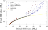Fig. 3 Mass scatter diagram for M⋆ = 106 M⊙, rc,⋆ = 1 pc, star formation efficiency ε = 0.35, and one run.

Fig. 4 Final BH spin probability density function for M⋆ = 106 M⊙, rc,⋆ = 1 pc, star formation efficiency ε = 0.35, and ten runs.

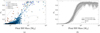Fig. 5 Final BH spin with respect to final BH mass for our typical cluster with M⋆ = 106 M⊙, rc,⋆ = 1 pc, and a star formation efficiency of ε = 0.35. (a) Scatter diagram for one indicative run. We have circled {high-spin, low-mass} and {low-spin, high-mass} outliers. (b) Percentiles, median, and fit relation, expressed by Eq. (31), for ten runs.

5 Conclusion

We calculated the BH spin distribution generated by accretion in gaseous proto-stellar clusters within ~10 Myr as gas is exponentially depleted by stellar feedback. We mainly considered parameter values consistent with JWST observations of five proto-stellar clusters in the Cosmic Gems arc galaxy (Adamo et al. 2024) and also explored a broader parameter space.

Our accretion model incorporates the repeated disruption of BH accretion disks by gravitational perturbations in dense cluster environments. The disk orientation is determined by the acquired BH’s azimuthal velocity, and therefore each disruption reorients the disk. Our major results are summarized in Tables 1 and 2, Fig. 5b, and Eq. (31).

This equation describes a BH spin distribution as a function of BH mass with a remarkably consistent functional form; it persists for all cluster parameter values investigated here, with representative ranges given in Table 1. This behavior, depicted graphically in Fig. 5b, reveals a spin-mass correlation with three regimes: low spins (a_* ≲ 0.3) for low BH masses, a steep increase with a transition mass scale of ~50 M_⊙ and a corresponding spin of ~0.5, and a saturating plateau for high masses.

For the typical Cosmic Gems cluster mass, 10⁶ M_⊙, and size, 1 pc, the saturating spin reaches a median value of ${\overline{a}}_{\ast }^{\text{sat}}=0.90$ for m_BH ≥ 100 M_⊙, with the 1σ range covering a_* = 0.70 − 0.96 (see Table 1). Remarkably, these BH spin values and corresponding masses are in good agreement with GW231123 (Abac et al. 2025), suggesting that some heavy BHs within the upper BH mass gap could have formed via accretion within the first compact massive stellar clusters, during their formation stage in the early Universe.

Our predicted spin-mass correlation is most likely to survive in clusters that later evolve into GCs, where repeated mergers are expected to be inefficient. By contrast, if the cluster migrates to, or is formed inside, the galactic nucleus and becomes part of a NSC, repeated mergers may erase the correlation, depending mainly on the merger timescales and the growth history of the NSC.

Finally, we stress that the stochastic nature of the process also underlies the presence of low-spin, high-mass outliers for sufficiently massive clusters representative of the Cosmic Gems population. Specifically, we expect ~ 1 mass-gap BH per cluster with a low spin of a_* ≲ 0.1. Massive BHs (m_BH ≳ 500 M_⊙) with a low spin of a_* ≲ 0.3 are significantly rarer but cannot be excluded.

Thus, our proposed BH spin and mass growth channel has two distinctive signatures: primarily, the spin-mass correlation of Fig. 5b, mathematically expressed by the characteristic saturating exponential profile of the BH spin distribution, as in Eq. (31); second, the presence of low-spin, high-mass BH outliers, which are difficult to explain with the repeated-merger channel. Possible important avenues for future work include (i) the analysis of GW data to identify potential candidates of our proposed channel based on these two signatures, and to distinguish them from those produced by the repeated-merger channel; (ii) the calculation of the contribution to the GW background generated by accreting BBHs in such gaseous proto-stellar clusters; and (iii) the calculation of IMBH binary merger rates in these environments, which is important for the planned LISA mission.

Acknowledgements

Z.R. is supported by the European Union’s Horizon Europe Research and Innovation Programme under the Marie Skłodowska-Curie grant agreement No. 101149270–ProtoBH.

References

Appendix A Stochastic kick timesteps

Our estimate of the stochastic timestep Δt_stoch for applying velocity increments onto each BH relies on a coarse-grained description of the unresolved perturbations experienced by the BH as it moves through the local stellar and gaseous background. In this picture the natural reference timescale is the gravitational dynamical timescale ${\tau }_{\text{grav}}\left(r_{•}\right)=\sqrt{r_{•}^3/G{M}_{\text{enc}}(r_{•})}$, while additional timescales are used as consistency bounds. Our code calculates the adaptive local timestep for each BH as $$\mathrm{\Delta }{t}_{\mathrm{s}\mathrm{t}\mathrm{o}\mathrm{c}\mathrm{h}}=f_{\mathrm{d}\mathrm{t}}\cdot min\{{\tau }_{\mathrm{g}\mathrm{r}\mathrm{a}\mathrm{v}},{\tau }_{\mathrm{d}\mathrm{f}},{\tau }_{\mathrm{c}\mathrm{r}\mathrm{o}\mathrm{s}\mathrm{s}},{\tau }_{\mathrm{t}\mathrm{u}\mathrm{r}\mathrm{b}}\},$$(A.1)

where we denote the dynamical friction timescale τ_df = 1/(η_•,⋆ + η_•,gas), the core crossing time τ_cross = r_c,⋆/v_•, the supersonic turbulence correlation time τ_turb = r_c,gas/(2c_s,gas) and a control parameter f_dt. The dynamical friction coefficient behaves as ${\eta }_{•}\propto 4\pi m_{•}{G}^2\rho /v_{•}^3$; in particular we use the standard Chandrasekhar formula for the star component and the prescription of Ostriker (1999) for the gas component (see Paper I for details). Here c_s,gas denotes the sound speed of the ambient cluster gas, not of the accretion disk gas.

There is a hierarchy behind Eq. (A.1). Dynamical friction is a cumulative relaxation process for each BH and therefore should operate on a timescale longer than the local dynamical time. It is natural then to update the stochastic forcing on the timescale over which the local perturber population evolves, Δt_stoch = 𝒪(τ_grav), as long as τ_df ≫ τ_grav. In all our runs we have typically τ_grav ≲ 10⁻² τ_df, and at least τ_grav < 10⁻¹ τ_df, throughout the whole time evolution, as illustrated in Fig. A.1 for two represantive BHs of different mass. Accordingly, τ_grav sets the stochastic timestep for ~99% of all kicks for BHs with final mass m_• ≥ 15M_⊙ and for the vast majority ≳ 75% of BHs with lower final masses. The crossing time τ_cross becomes relevant only for low-mass BHs displaced to the outskirts of the core after a previous strong kick, but still getting τ_cross ≈ τ_grav in those cases. The τ_turb remains always larger than τ_grav for our adopted turbulence Mach number ℳ_turb = 2, and more generally for any ℳ_turb ≲ 10. We also implemented in the code prescribed bounds on Δt_stoch to improve numerical stability, which nevertheless were never violated by Eq. (A.1) in practice.

Furthermore, in order to account for the approximate nature of Δt_stoch we introduce the numerical control parameter f_dt. For the simulations presented here, we adopt the value f_dt = 0.5, resolving the stochastic updates more finely than the local dynamical timescale without oversampling the coarse-grained evolution. We also explored the parameter range f_dt = 0.1–2.0 and found that our primary results on the BH spin-mass correlation are robust under this variation. In particular, the general spin-mass trend remains the same. The difference is that a longer timestep tends to broaden the spread of spin values resulting in a median saturation spin at high masses smaller by ~ 10% or less for f_dt = 2.0 with respect to f_dt = 0.5. Nevertheless, similar maximum spin values are achieved.

Among heavy BHs with m_•,f ≥ 50 M_⊙, the Δt_stoch presents negligible variation throughout the cluster evolution. Lower-mass BHs show a larger spread, because they receive larger velocity kicks and also are born at different times (originating in diverse stelar evolution channels). This is manifested as a sharp broadening of their distribution depicted in Fig. A.2, where we plot the evolution of the median $\tilde{\mathrm{\Delta }}{t}_{\text{stoch}}$ and the 1σ percentile for light and heavy BHs. Still, for all BHs, it is Δt_stoch = 𝒪(10⁻² Myr) varying less than half an order of magnitude. This is true also for all cluster parameters inspected here, with lower compactness at the same cluster mass leading to slightly higher Δt_stoch, but still of the same order of magnitude.

Fig. A.1 The evolution of timescales used in Eq. (A.1) for two heavy BHs grown to final masses (a) 100 M⊙ and (b) 985 M⊙, in an indicative run of our typical cluster M⋆ = 106 M⊙, rc,⋆ = 1 pc ε = 0.35.

Fig. A.2 Evolution of the median stochastic timestep $\tilde{\mathrm{\Delta }}{t}_{\text{stoch}}$ and its 1σ percentile for final low-mass (10 − 50 M⊙) and heavy (> 50 M⊙) BHs. Two runs of a cluster as in Fig. A.1.

Finally, we remark that heavy BHs tend to receive more kicks than lower-mass BHs, having shorter stochastic timesteps and being born mostly earlier in cluster’s life. For our typical massive compact cluster, M_⋆ = 10⁶ M_⊙, r_c,⋆ = 1 pc, we report the median, the range and 1σ percentile (in parenthesis) of stochastic cycles for several masses as follows: (i) the BHs which have grown massive, (150 − 10³) M_⊙, have received $\approx {1400}_{-200(120)}^{+180(130)}$ kicks, (ii) the BHs with final mass within the mass gap, (50 − 150) M_⊙, have received $\approx {1300}_{-190(120)}^{+290(170)}$ kicks, (iii) the low-mass BHs, m_•,f < 50 M_⊙, have received $\approx {600}_{-500(260)}^{+990(300)}$ kicks. The primary cluster parameter that determines the stochastic cycles is the cluster compactness rather than the cluster mass. Less compact clusters that can drive BH mass growth only up to m_•,max ≲ 150 M_⊙ generate ~ 25% less number of kicks per BH.

Appendix B Accretion disk timescales

Warp timescale.. The outer radius (25) of the accretion disk at which the warp propagates is defined by the condition t_w(R_out) = Δt_stoch, where t_w(R) is the local warp-propagation timescale. For thin disks, warp communication occurs diffusively (Frank et al. 2002), with a radial diffusion timescale (Pringle 1992) (see also Lodato & Pringle 2007) $$t_{\mathrm{w}}^{(\text{thin)\hspace{0.17em}}}(R)\sim \frac{R^2}{{\nu }_2}=2\mathrm{s}{\left(\frac{f_{{\nu }_2}}{0.6}\right)}^{-1}{\left(\frac{\alpha }{0.1}\right)}^{\frac{6}{5}}{\dot{m}}^{-\frac{3}{10}}{\left(\frac{m_{\mathrm{B}\mathrm{H}}}{50{\mathrm{M}}_{\odot }}\right)}^{\frac{6}{5}}{\left(\frac{R}{r_{\mathrm{g}}}\right)}^{\frac{5}{4}}$$(B.1)

where ν₂ is the transverse viscosity and f_ν2 a coefficient determined in simulations depending on α (Perego et al. 2009). We use the value f_v2 = 0.6 appropriate for the value α = 0.1 that we use for thin disks.

For slim disks, which belong to the bending-wave regime (α < H/R), warping disturbances propagate on a timescale (Nelson & Papaloizou 1999) $$t_{\mathrm{w}}^{(\mathrm{s}\mathrm{l}\mathrm{i}\mathrm{m})}(R)\sim \frac{2R}{c_{s,\text{disk}}}=4.9\cdot {10}^{-3}\mathrm{s}{\left(\frac{H/R}{0.1}\right)}^{-1}\left(\frac{m_{\mathrm{B}\mathrm{H}}}{50{\mathrm{M}}_{\odot }}\right){\left(\frac{R}{r_{\mathrm{g}}}\right)}^{\frac{3}{2}}$$(B.2)

where c_s,disk ≈ HΩ_K,disk(R).

BH-alignment timescale.. We calculate the BH-alignment timescale (t_al,•) that is the typical time required for the BH to align with the disk (case J_d/(2J_BH) > 1). This is determined by the gravitomagnetic timescale, t_gm, of the torque exerted by the disk onto the BH $$t_{\mathrm{g}\mathrm{m}}(R)\sim \frac{c^2}{4\pi G}\frac{1}{\sum (R){\mathrm{\Omega }}_{\mathrm{K},•}(R)R}$$(B.3)

at the distance of maximum torque R_T. It is (Martin et al. 2007) $$t_{\mathrm{a}\mathrm{l},•}\sim \sqrt{2}{t}_{\mathrm{g}\mathrm{m}}\left(R_{\mathrm{T}}\right)=17.9\mathrm{y}\mathrm{r}{\left(\frac{\alpha }{0.01}\right)}^{\frac{4}{5}}{\left(\frac{m_{\mathrm{B}\mathrm{H}}}{50{\mathrm{M}}_{\odot }}\right)}^{\frac{4}{5}}{\left(\frac{R_{\mathrm{T}}}{r_{\mathrm{g}}}\right)}^{\frac{5}{4}}{\dot{m}}^{-\frac{7}{10}}.$$(B.4)

In the thin-disk case, the radius of maximum torque is the “warp” or “Bardeen–Petterson” radius defined as the distance at which the warp timescale (B.1) equals the Lense–Thirring precession timescale ${\mathrm{\Omega }}_{\mathrm{L}\mathrm{T}}^{-1}$, that is $R_{\mathrm{T}}^{(\text{thin})}\sim \frac{4\pi G{J}_{\mathrm{B}\mathrm{H}}}{{\nu }_2{c}^2}$ which gives $$\frac{R_{\mathrm{T}}^{(\text{thin\hspace{0.17em}})}}{r_{\mathrm{g}}}\sim 374.3a_{\ast }^{\frac{4}{7}}{\left(\frac{f_{{\nu }_2}}{0.6}\right)}^{-\frac{4}{7}}{\left(\frac{\alpha }{0.1}\right)}^{\frac{24}{35}}{\dot{m}}^{-\frac{6}{35}}{\left(\frac{m_{\mathrm{B}\mathrm{H}}}{50{\mathrm{M}}_{\odot }}\right)}^{\frac{4}{35}}.$$(B.5)

Substituting in (B.4) we get $$\frac{t_{\mathrm{a}\mathrm{l},•}^{(\mathrm{t}\mathrm{h}\mathrm{i}\mathrm{n})}}{\mathrm{\Delta }{t}_{\mathrm{s}\mathrm{t}\mathrm{o}\mathrm{c}\mathrm{h}}}\sim 18a_{\ast }^{\frac{5}{7}}{\left(\frac{\mathrm{\Delta }{t}_{\mathrm{s}\mathrm{t}\mathrm{o}\mathrm{c}\mathrm{h}}}{{10}^{-2}\mathrm{M}\mathrm{y}\mathrm{r}}\right)}^{-1}{\left(\frac{f_{v_2}}{0.6}\right)}^{-\frac{5}{7}}{\left(\frac{\alpha }{0.1}\right)}^{\frac{58}{35}}{\left(\frac{m_{\mathrm{B}\mathrm{H}}}{50{\mathrm{M}}_{\odot }}\right)}^{\frac{-2}{35}}{\dot{m}}^{-\frac{32}{35}}.$$(B.6)

In practice, this timescale is mostly irrelevant since the case J_d/(2J_BH) > 1 refers primarily to more massive BHs for which $\dot{m}>0.3$, i.e. slim disks (see Eq. 24).

In the slim-disk case (bending-wave α < H/R) the maximum torque is applied at a distance (King et al. 2005) $$\frac{R_{\mathrm{T}}^{(\mathrm{s}\mathrm{l}\mathrm{i}\mathrm{m})}}{r_{\mathrm{g}}}\sim 3.6a_{\ast }^{\frac{2}{5}}(H/R{)}^{-\frac{4}{5}}.$$(B.7)

Substituting in (B.4) we get $$\frac{t_{\text{al\hspace{0.17em}},•}^{(\text{slim\hspace{0.17em}})}}{\mathrm{\Delta }{t}_{\text{stoch\hspace{0.17em}}}}\sim 0.09a_{\ast }^{\frac{1}{2}}{\left(\frac{\mathrm{\Delta }{t}_{\text{stoch\hspace{0.17em}}}}{{10}^{-2}\mathrm{M}\mathrm{y}\mathrm{r}}\right)}^{-1}{\left(\frac{H/R}{0.1}\right)}^{-1}{\left(\frac{\alpha }{0.01}\right)}^{\frac{4}{5}}{\left(\frac{m_{\mathrm{B}\mathrm{H}}}{50{\mathrm{M}}_{\odot }}\right)}^{\frac{4}{5}}{\dot{m}}^{-\frac{7}{10}}.$$(B.8)

We see that massive BHs within the mass gap, m_BH ≲ 150M_⊙, satisfy $t_{\mathrm{a}\mathrm{l},•}^{(\mathrm{s}\mathrm{l}\mathrm{i}\mathrm{m})}\lesssim 0.1\mathrm{\Delta }{t}_{\text{stoch\hspace{0.17em}}}$ even at high spin a_* ≈ 0.9 and sufficiently high accretion rate $\dot{m}\gtrsim 1$.

Note that when the BH dominates the angular momentum, J_d/(2J_BH) < 1, it is the inner disk which reorients itself to (or counter to) the BH spin. In this case, Eqs. (B.1) or (B.2), for the thin or slim disk respectively, should be used (instead of Eq. B.4) substituting R with an inner radius R_in ≈ R_ISCO. This yields t_al,d ≪ Δt_stoch for the parameter space of our study.

All Tables

All Figures

	Fig. 1 Depletion timescale, τ, with respect to the compactness, C, of a gaseous stellar cluster of any total mass at low metallicity (~0.01Z⊙) for different possible star formation efficiencies, ε.
In the text

	Fig. 2 Contour of the median stochastic timestep, $\tilde{\mathrm{\Delta }}{t}_{\text{stoch}}$, with respect to the median BH position, ${\tilde{r}}_{\mathrm{B}\mathrm{H}}$, and the final BH mass, mBH,f, for an indicative run of our typical cluster, M⋆ = 106 M⊙, rc,⋆ = 1 pc ε = 0.35.
In the text

	Fig. 3 Mass scatter diagram for M⋆ = 106 M⊙, rc,⋆ = 1 pc, star formation efficiency ε = 0.35, and one run.
In the text

	Fig. 4 Final BH spin probability density function for M⋆ = 106 M⊙, rc,⋆ = 1 pc, star formation efficiency ε = 0.35, and ten runs.
In the text

	Fig. 5 Final BH spin with respect to final BH mass for our typical cluster with M⋆ = 106 M⊙, rc,⋆ = 1 pc, and a star formation efficiency of ε = 0.35. (a) Scatter diagram for one indicative run. We have circled {high-spin, low-mass} and {low-spin, high-mass} outliers. (b) Percentiles, median, and fit relation, expressed by Eq. (31), for ten runs.
In the text

	Fig. A.1 The evolution of timescales used in Eq. (A.1) for two heavy BHs grown to final masses (a) 100 M⊙ and (b) 985 M⊙, in an indicative run of our typical cluster M⋆ = 106 M⊙, rc,⋆ = 1 pc ε = 0.35.
In the text

	Fig. A.2 Evolution of the median stochastic timestep $\tilde{\mathrm{\Delta }}{t}_{\text{stoch}}$ and its 1σ percentile for final low-mass (10 − 50 M⊙) and heavy (> 50 M⊙) BHs. Two runs of a cluster as in Fig. A.1.
In the text

References

- Abac, A. G., Abouelfettouh, I., Acernese, F., et al. 2025, ApJ, 993, L25 [Google Scholar]
- Abbott, R., Abbott, T. D., Acernese, F., et al. 2023, Phys. Rev. X, 13, 041039 [Google Scholar]
- Adamo, A., Bradley, L. D., Vanzella, E., et al. 2024, Nature, 632, 513 [NASA ADS] [CrossRef] [Google Scholar]
- Antonini, F., Gieles, M., & Gualandris, A. 2019, MNRAS, 486, 5008 [NASA ADS] [CrossRef] [Google Scholar]
- Arca Sedda, M., Kamlah, A. W. H., Spurzem, R., et al. 2023, MNRAS, 526, 429 [NASA ADS] [CrossRef] [Google Scholar]
- Baibhav, V., Gerosa, D., Berti, E., et al. 2020, Phys. Rev. D, 102, 043002 [NASA ADS] [CrossRef] [Google Scholar]
- Bardeen, J. M., Press, W. H., & Teukolsky, S. A. 1972, ApJ, 178, 347 [Google Scholar]
- Bartos, I., & Haiman, Z. 2025, arXiv e-prints [arXiv:2508.08558] [Google Scholar]
- Baumgardt, H., & Kroupa, P. 2007, MNRAS, 380, 1589 [NASA ADS] [CrossRef] [Google Scholar]
- Baumgardt, H., & Makino, J. 2003, MNRAS, 340, 227 [NASA ADS] [CrossRef] [Google Scholar]
- Baumgarte, T. W., & Shapiro, S. L. 2025, Phys. Rev. D, 111, 063039 [Google Scholar]
- Belczynski, K., Heger, A., Gladysz, W., et al. 2016, Astron. Astrophys., 594, A97 [Google Scholar]
- Benacquista, M. J., & Downing, J. M. B. 2013, Liv. Rev. Relativ., 16, 4 [NASA ADS] [CrossRef] [Google Scholar]
- Bisnovatyi-Kogan, G. S., & Ruzmaikin, A. A. 1974, Ap&SS, 28, 45 [NASA ADS] [CrossRef] [Google Scholar]
- Bonnell, I. A., Clarke, C. J., Bate, M. R., & Pringle, J. E. 2001, MNRAS, 324, 573 [NASA ADS] [CrossRef] [Google Scholar]
- Corsaro, E., Lee, Y.-N., García, R. A., et al. 2017, Nat. Astron., 1, 0064 [NASA ADS] [CrossRef] [Google Scholar]
- Elmegreen, B. G. 2018, ApJ, 869, 119 [NASA ADS] [CrossRef] [Google Scholar]
- Fishbach, M., Holz, D. E., & Farr, B. 2017, ApJL, 840, L24 [Google Scholar]
- Frank, J., King, A., & Raine, D. J. 2002, Accretion Power in Astrophysics. 3rd edn. (Cambridge: Cambridge University Press) [Google Scholar]
- Fujii, M. S., Wang, L., Tanikawa, A., Hirai, Y., & Saitoh, T. R. 2024, Science, 384, 1488 [NASA ADS] [CrossRef] [Google Scholar]
- Fuller, J., & Ma, L. 2019, ApJL, 881, L1 [Google Scholar]
- Gammie, C. F., Shapiro, S. L., & McKinney, J. C. 2004, ApJ, 602, 312 [NASA ADS] [CrossRef] [Google Scholar]
- Gerosa, D., & Berti, E. 2017, Phys. Rev. D, 95, 124046 [NASA ADS] [CrossRef] [Google Scholar]
- Gerosa, D., & Berti, E. 2019, Phys. Rev. D, 100, 041301 [NASA ADS] [CrossRef] [Google Scholar]
- Gottlieb, O., Metzger, B. D., Issa, D., et al. 2025, ApJL, 993, L54 [Google Scholar]
- Groh, J. H., Ekström, S., Georgy, C., et al. 2019, Astron. Astrophys., 627, A24 [Google Scholar]
- Healy, B. F., McCullough, P. R., Schlaufman, K. C., & Kovacs, G. 2023, ApJ, 944, 39 [NASA ADS] [CrossRef] [Google Scholar]
- Inayoshi, K., Haiman, Z., & Ostriker, J. P. 2016, MNRAS, 459, 3738 [NASA ADS] [CrossRef] [Google Scholar]
- Jackson, R. J., & Jeffries, R. D. 2010, MNRAS, 402, 1380 [NASA ADS] [CrossRef] [Google Scholar]
- Kimball, C., Talbot, C. L., Berry, C. P., et al. 2020, ApJ, 900, 177 [NASA ADS] [CrossRef] [Google Scholar]
- King, A. R., & Pringle, J. E. 2006, MNRAS, 373, L90 [NASA ADS] [CrossRef] [Google Scholar]
- King, A. R., Lubow, S. H., Ogilvie, G. I., & Pringle, J. E. 2005, MNRAS, 363, 49 [NASA ADS] [CrossRef] [Google Scholar]
- King, A. R., Pringle, J. E., & Hofmann, J. A. 2008, MNRAS, 385, 1621 [NASA ADS] [CrossRef] [Google Scholar]
- Kıroğlu, F., Kremer, K., & Rasio, F. A. 2025, ApJ, 994, L37 [Google Scholar]
- Krause, M., Fierlinger, K., Diehl, R., et al. 2013, Astron. Astrophys., 550, A49 [Google Scholar]
- Krause, M. G. H., Charbonnel, C., Bastian, N., & Diehl, R. 2016, Astron. Astrophys., 587, A53 [Google Scholar]
- Kruijssen, J. M. D. 2015, MNRAS, 454, 1658 [Google Scholar]
- Kudritzki, R. P. 2002, ApJ, 577, 389 [NASA ADS] [CrossRef] [Google Scholar]
- Lada, C. J., & Lada, E. A. 2003, Ann. Rev. Astron. Astrophys., 41, 57 [Google Scholar]
- Lee, S., Lee, H. M., Kim, J.-h., et al. 2025, ApJ, 988, 15 [Google Scholar]
- Leigh, N. W. C., Mastrobuono-Battisti, A., Perets, H. B., & Böker, T. 2014, MNRAS, 441, 919 [NASA ADS] [CrossRef] [Google Scholar]
- Levin, Y. 2007, MNRAS, 374, 515 [Google Scholar]
- Liu, S., Wang, L., Tanikawa, A., Wu, W., & Fujii, M. S. 2025, ApJ, 993, L30 [Google Scholar]
- Lodato, G., & Pringle, J. E. 2007, MNRAS, 381, 1287 [Google Scholar]
- Mapelli, M., Dall’Amico, M., Bouffanais, Y., et al. 2021, MNRAS, 505, 339 [CrossRef] [Google Scholar]
- Martin, R. G., Pringle, J. E., & Tout, C. A. 2007, MNRAS, 381, 1617 [NASA ADS] [CrossRef] [Google Scholar]
- McKernan, B., Ford, K. E. S., Lyra, W., & Perets, H. B. 2012, MNRAS, 425, 460 [NASA ADS] [CrossRef] [Google Scholar]
- Merritt, D. 2013, Dynamics and Evolution of Galactic Nuclei, Princeton Series in Astrophysics (Princeton: Princeton University Press) [Google Scholar]
- Miller, M. C., & Hamilton, D. P. 2002, MNRAS, 330, 232 [Google Scholar]
- Nealon, R., Price, D. J., & Nixon, C. J. 2015, MNRAS, 448, 1526 [NASA ADS] [CrossRef] [Google Scholar]
- Nelson, R. P., & Papaloizou, J. C. B. 1999, MNRAS, 309, 929 [CrossRef] [Google Scholar]
- Nixon, C., King, A., Price, D., & Frank, J. 2012, ApJL, 757, L24 [Google Scholar]
- O’Leary, R. M., Rasio, F. A., Fregeau, J. M., Ivanova, N., & O’Shaughnessy, R. 2006, ApJ, 637, 937 [CrossRef] [Google Scholar]
- Ostriker, E. C. 1999, ApJ, 513, 252 [Google Scholar]
- Paczyński, B. 1971, Ann. Rev. Astron. Astrophys., 9, 183 [Google Scholar]
- Penna, R. F., McKinney, J. C., Narayan, R., et al. 2010, MNRAS, 408, 752 [NASA ADS] [CrossRef] [Google Scholar]
- Perego, A., Dotti, M., Colpi, M., & Volonteri, M. 2009, MNRAS, 399, 2249 [NASA ADS] [CrossRef] [Google Scholar]
- Perna, R., Wang, Y.-H., Farr, W. M., Leigh, N., & Cantiello, M. 2019, ApJL, 878, L1 [Google Scholar]
- Pringle, J. E. 1992, MNRAS, 258, 811 [NASA ADS] [CrossRef] [Google Scholar]
- Puls, J., Vink, J. S., & Najarro, F. 2008, Astron. Astrophys.Rev., 16, 209 [Google Scholar]
- Purohit, R. A., Fragione, G., Rasio, F. A., Petter, G. C., & Hickox, R. C. 2024, AJ, 167, 191 [Google Scholar]
- Renzini, A. 2017, MNRAS, 469, L63 [Google Scholar]
- Renzo, M., Ott, C. D., Shore, S. N., & de Mink, S. E. 2017, Astron. Astrophys., 603, A118 [Google Scholar]
- Renzo, M., Cantiello, M., Metzger, B. D., & Jiang, Y. F. 2020, ApJL, 904, L13 [Google Scholar]
- Reynolds, C. S. 2021, Ann. Rev. Astron. Astrophys., 59, 117 [Google Scholar]
- Ricarte, A., Narayan, R., & Curd, B. 2023, ApJL, 954, L22 [Google Scholar]
- Rizzuto, F. P., Naab, T., Spurzem, R., et al. 2022, MNRAS, 512, 884 [NASA ADS] [CrossRef] [Google Scholar]
- Rodriguez, C. L., Chatterjee, S., & Rasio, F. A. 2016, Phys. Rev. D, 93, 084029 [NASA ADS] [CrossRef] [Google Scholar]
- Roupas, Z. 2021, Astron. Astrophys., 646, A20 [Google Scholar]
- Roupas, Z. 2025, Astron. Astrophys., 702, A208 [Google Scholar]
- Roupas, Z., & Kazanas, D. 2019, Astron. Astrophys., 632, L8 [Google Scholar]
- Ruffert, M., & Anzer, U. 1995, Astron. Astrophys., 295, 108 [Google Scholar]
- Safarzadeh, M., & Haiman, Z. 2020, ApJL, 903, L21 [Google Scholar]
- Sander, A. A. C., & Vink, J. S. 2020, MNRAS, 499, 873 [Google Scholar]
- Shakura, N. I., & Sunyaev, R. A. 1973, Astron. Astrophys., 24, 337 [Google Scholar]
- Sądowski, A. 2009, Astrophys. J. Supp., 183, 171 [Google Scholar]
- Sądowski, A., Abramowicz, M., Bursa, M., et al. 2011a, Astron. Astrophys., 527, A17 [Google Scholar]
- Sądowski, A., Bursa, M., Abramowicz, M., et al. 2011b, Astron. Astrophys., 532, A41 [Google Scholar]
- Spera, M., & Mapelli, M. 2017, MNRAS, 470, 4739 [Google Scholar]
- Spitzer, L. 1987, Dynamical Evolution of Globular Clusters (Princeton: Princeton University Press) [Google Scholar]
- Spruit, H. C. 2002, Astron. Astrophys., 381, 923 [Google Scholar]
- Tchekhovskoy, A., Narayan, R., & McKinney, J. C. 2011, MNRAS, 418, L79 [NASA ADS] [CrossRef] [Google Scholar]
- Thorne, K. S. 1974, ApJ, 191, 507 [Google Scholar]
- Torniamenti, S., Mapelli, M., Périgois, C., et al. 2024, Astron. Astrophys., 688, A148 [Google Scholar]
- Tripathi, P. K., Chattopadhyay, I., & Joshi, R. K. 2025, ApJ, 979, 61 [Google Scholar]
- Vink, J. S., de Koter, A., & Lamers, H. J. G. L. M. 2001, Astron. Astrophys., 369, 574 [Google Scholar]
- Woosley, S. E., & Heger, A. 2021, ApJL, 912, L31 [Google Scholar]
- Yang, Y., Gayathri, V., Bartos, I., et al. 2020, ApJL, 901, L34 [Google Scholar]
- Yi, S.-X., Cheng, K. S., & Taam, R. E. 2018, ApJL, 859, L25 [Google Scholar]