| Issue |
A&A
Volume 709, May 2026
|
|
|---|---|---|
| Article Number | A244 | |
| Number of page(s) | 12 | |
| Section | Catalogs and data | |
| DOI | https://doi.org/10.1051/0004-6361/202659177 | |
| Published online | 22 May 2026 | |
The CARMENES search for exoplanets around M dwarfs
A homogeneous catalogue of projected rotational velocities accounting for limb darkening
1
Instituto de Astrofísica de Andalucía, CSIC, Glorieta de la Astronomía s/n,
18008
Granada,
Spain
2
INAF – Palermo Astronomical Observatory,
Piazza del Parlamento, 1,
90134
Palermo,
Italy
3
Institut für Astrophysik und Geophysik, Georg-August-Universität Göttingen,
Friedrich-Hund-Platz 1,
37077
Göttingen,
Germany
4
Centro de Astrobiología, CSIC-INTA, Camino Bajo del Castillo s/n, Campus ESAC,
28692
Villanueva de la Cañada, Madrid,
Spain
5
Universidad de Granada,
c/ Gran Vía de Colón 48,
18010
Granada,
Spain
6
Landessternwarte, Zentrum für Astronomie der Universität Heidelberg,
Königstuhl 12,
69117
Heidelberg,
Germany
7
Institut de Ciències de l’Espai, CSIC, c/ de Can Magrans s/n, Campus UAB,
08193
Bellaterra, Barcelona,
Spain
8
Institut d’Estudis Espacials de Catalunya,
08860
Castelldefels, Barcelona,
Spain
9
Instituto de Astrofísica de Canarias,
38205
La Laguna, Tenerife,
Spain
10
Departamento de Astrofísica, Universidad de La Laguna,
38206
La Laguna, Tenerife,
Spain
11
Departamento de Física de la Tierra y Astrofísica & IPARCOS Instituto de Física de Partículas y del Cosmos, Facultad de Ciencias Físicas, Universidad Complutense de Madrid,
Plaza de Ciencias 1,
28400
Madrid,
Spain
12
Thüringer Landessternwarte Tautenburg,
Sternwarte 5,
07778
Tautenburg,
Germany
13
Max-Planck-Institut für Astronomie,
Königstuhl 17,
69117
Heidelberg,
Germany
14
Centro Astronómico Hispano en Andalucía, Observatorio Astronómico de Calar Alto, Sierra de los Filabres,
04550
Gérgal, Almería,
Spain
15
Hamburger Sternwarte,
Gojenbergsweg 112,
21029
Hamburg,
Germany
★ Corresponding author: This email address is being protected from spambots. You need JavaScript enabled to view it.
Received:
28
January
2026
Accepted:
10
April
2026
Abstract
Stellar rotation is closely linked to both the age and the magnetic activity of stars. Through gyrochronology, studying stellar rotation provides a means to estimate stellar ages and trace the evolution of planetary systems, and it is also a crucial means to constrain and correct stellar activity effects for robust exoplanet detection and characterisation. CARMENES is a dual-channel, high-resolution (ℛ > 80 000) spectrograph that has been highly successful in detecting exoplanets around M-dwarf stars using the radial-velocity technique, and it also enables precise measurements of the projected rotational velocity (v sin i) from spectral line broadening. We present an oversampled convolution method that incorporates a realistic limb-darkening model to determine v sin i from CARMENES spectra by comparing observed spectra with that of a template star. The advantages over existing methods in the literature have been assessed using high-resolution synthetic spectrat that span effective temperatures of 2500–4000 K and projected rotational velocities of up to 50 km s−1. We applied our method to 392 M dwarfs observed with CARMENES and it yielded v sin i measurements (or upper limits at 2 km s−1) with a median relative uncertainty of 6.8%, which is substantially smaller than the 15.4% reported in the literature. This work provides the largest uniform catalogue of v sin i measurements for M dwarfs, including significantly updated values for several targets, along with 36 new targets.
Key words: methods: numerical / techniques: spectroscopic / stars: activity / stars: late-type / stars: rotation
© The Authors 2026
 Open Access article, published by EDP Sciences, under the terms of the Creative Commons Attribution License (https://creativecommons.org/licenses/by/4.0), which permits unrestricted use, distribution, and reproduction in any medium, provided the original work is properly cited.
This article is published in open access under the Subscribe to Open model. This email address is being protected from spambots. You need JavaScript enabled to view it. to support open access publication.
1 Introduction
M-dwarf stars are the most numerous stellar population in our Galaxy, constituting roughly 75% of stars in the solar neighbourhood (Henry et al. 2006, 2018). Their small sizes and masses (0.61–0.075 M⊙; Henry & Jao 2024), low temperatures (3900–2300 K; Cifuentes et al. 2020), and long lifetimes make them prime targets for the detection of small, temperate exoplanets (Bonfils et al. 2013; Sabotta et al. 2021). Characterising the rotation of M dwarfs provides information about their magnetic activity, internal structure, and age (Suárez Mascareño et al. 2015; Newton et al. 2016; Díez Alonso et al. 2019; Shan et al. 2024). These constraints are essential for interpreting the formation and evolution of their planetary systems.
The Calar Alto high-Resolution search for M dwarfs with Exoearths using Near-infrared and optical Echelle Spectrographs (CARMENES1) project provides an excellent dataset for improving rotational velocity measurements in M dwarfs. CARMENES is a dual-channel spectrograph (VIS; 520–960 nm; NIR: 960–1710 nm) with a high spectral resolution (ℛ = 94 600 and ℛ = 80 400, respectively), mounted on the 3.5 m telescope at the Calar Alto Observatory (CAHA) in Almería, Spain (Quirrenbach et al. 2014, 2018). The survey has delivered high-quality spectra and radial-velocity (RV) time series for nearly 400 nearby M dwarfs (Ribas et al. 2023), which has enabled the discovery of numerous exoplanets as well as detailed studies of stellar rotation, activity, and variability (Baroch et al. 2020; Jeffers et al. 2022; Fuhrmeister et al. 2018, 2023; Shan et al. 2024; Ruh et al. 2024).
A fundamental measure of stellar rotation is the projected rotational velocity, v sin i, which represents a star’s equatorial rotation along the line of sight. It is typically inferred from the Doppler broadening of absorption lines in high-resolution spectra. Determining v sin i accurately is challenging, as rotational broadening must be disentangled from other line-broadening mechanisms, such as instrumental effects and stellar turbulence. Conventional approaches often approximate the rotational profile using a convolution kernel that accounts for limb darkening. However, most studies adopt a fixed linear limb-darkening coefficient (usually u = 0.6) that is independent of spectral type or wavelength (Jenkins et al. 2009; Reiners et al. 2012, 2022). As demonstrated in this work, this simplification can lead to systematic biases.
Our approach introduces two key enhancements to modelling rotational broadening. First, we applied an oversampled convolution to minimise numerical artefacts. Second, we adopted order-specific limb-darkened kernels that account for wavelength- and temperature-dependent linear coefficients. For each target and spectral order, we computed average u values from stellaratmosphere models and achieved higher fidelity across the full wavelength range. Tests based on synthetic spectra indicate that this method improves both the precision and accuracy of the results, while remaining computationally efficient.
We applied this method to 392 M dwarfs with CARMENES-VIS observations, which enabled us to make a direct comparison with previous studies based solely on VIS data. This application yielded a homogeneous catalogue2 of v sin i measurements. In Appendix A we discuss the prospects for extending the method to CARMENES-NIR data.
2 Observations and data reduction
2.1 CARMENES spectra
The CARMENES spectra were reduced using the caracal (CARMENES Reduction And CALibration) pipeline, as detailed by Caballero et al. (2016). Starting with the raw data, caracal performs dark and bias correction, order tracing, flat-relative optimal extraction, and wavelength calibration, which results in fully reduced and wavelength-calibrated 1D spectra.
The second pipeline is serval (SpEctrum Radial Velocity AnaLyser, Zechmeister et al. 2018). It creates a high signal-to-noise ratio spectrum using the reduced spectra of the target star. It then computes the series of RVs via least-square fitting, telluric masking, échelle order weighting, and correcting for systematic effects. The output also includes activity indices. Here we present the implementation in serval of the computation of the v sin i accounting for the effect of limb darkening.
2.2 Synthetic data
We adopted four spectra from the PHOENIX NewEra stellar atmosphere models (Hauschildt et al. 2025) and corresponding surface intensity distributions (Claret et al. 2025). The synthetic templates were selected from among main-sequence stars with solar metallicity, covering the range Teff = 2500–4000 K in steps of 500 K. Each template provides intensity spectra at 127 μ values, where μ is the cosine of the angle between the normal to the stellar surface and the line of sight, spanning the wavelength range 1000–60 000 Å with a constant step of 0.05 Å. These model spectra fully cover the CARMENES wavelength range at a slightly higher sampling rate than the instrument.
We numerically integrated the stellar spectrum over a grid of 3000 × 3000 square cells covering the sky-projected stellar disc, following the method described by Morello et al. (2022) and Canocchi et al. (2024). Each cell is identified by the Cartesian coordinates of its centre (xj; yj), which are normalized to the stellar radius. The corresponding μj values are calculated as
![Mathematical equation: $\[\mu_j=\sqrt{1-x_j^2-y_j^2}.\]$](/articles/aa/full_html/2026/05/aa59177-26/aa59177-26-eq1.png) (1)
(1)
The ‘static’ cell spectrum is then obtained by interpolation at μj from the template, here using a cubic spline, though the method is only weakly sensitive to the choice of interpolation scheme. To account for stellar rotation, we Doppler-shifted the spectrum of each cell according to its velocity along the line of sight,
![Mathematical equation: $\[v_j=\left(y_j ~\sin~ \bar{\lambda}-x_j ~\cos~ \bar{\lambda}\right) \cdot v ~\sin~ i,\]$](/articles/aa/full_html/2026/05/aa59177-26/aa59177-26-eq2.png) (2)
(2)
where ![Mathematical equation: $\[\bar{\lambda}\]$](/articles/aa/full_html/2026/05/aa59177-26/aa59177-26-eq3.png) is a dummy parameter in this context (we set
is a dummy parameter in this context (we set ![Mathematical equation: $\[\bar{\lambda}=0\]$](/articles/aa/full_html/2026/05/aa59177-26/aa59177-26-eq4.png) ). In the presence of a transiting planet,
). In the presence of a transiting planet, ![Mathematical equation: $\[\bar{\lambda}\]$](/articles/aa/full_html/2026/05/aa59177-26/aa59177-26-eq5.png) traditionally denotes the sky-projected spin-orbit angle. We resampled the Doppler-shifted spectra onto the same wavelength grid as the template through linear interpolation, allowing for the direct summation of the cell spectra.
traditionally denotes the sky-projected spin-orbit angle. We resampled the Doppler-shifted spectra onto the same wavelength grid as the template through linear interpolation, allowing for the direct summation of the cell spectra.
3 Methods
The rotational broadening of stellar spectra can be implemented using several approaches. The two most common ones are convolution with a rotational broadening kernel (Gray 2005) and direct numerical integration (Carvalho & Johns-Krull 2023). Although numerical integration provides a more general and potentially more accurate procedure, it is computationally more expensive. These methods are often adopted with a single linear limb-darkening coefficient (commonly u = 0.6), despite the fact that u depends on both stellar temperature and wavelength. In this work, we develop an oversampled convolution method that offers a fast and robust alternative while properly accounting for wavelength- and temperature-dependent limb darkening.
The following subsections describe the method and the incremental improvements, tested using synthetic spectra, that guided its development. The test setup consists of a disc-integrated reference spectrum with v sin i = 0 km s−1 and a rotationally broadened target spectrum with v sin i values of 4, 8, 14, 20, 30, and 50 km s−1, and effective temperatures of Teff = 2500, 3000, 3500, and 4000 K. These values are representative of the M-dwarf sample observed by CARMENES, although the method itself does not, in principle, impose any restriction on the stellar parameters. For each case, v sin i was computed using the linear limb-darkening law with theoretical u coefficients.
3.1 Classic convolution and grid-based v sin i fitting
The standard approach to determining v sin i involves convolving a chosen template spectrum with a rotational broadening kernel over a grid of trial v sin i values, and minimising the residuals with respect to the target spectrum. In this work, we adopted the commonly used semi-circular kernel, which represents a rigidly rotating, uniformly emitting stellar disc:
![Mathematical equation: $\[\tilde{K}(\tilde{v})=\sqrt{1-\tilde{v}^2},\]$](/articles/aa/full_html/2026/05/aa59177-26/aa59177-26-eq6.png) (3)
(3)
where ![Mathematical equation: $\[\tilde{v}\]$](/articles/aa/full_html/2026/05/aa59177-26/aa59177-26-eq7.png) is the velocity normalised to v sin i. The kernel was subsequently normalised to conserve flux.
is the velocity normalised to v sin i. The kernel was subsequently normalised to conserve flux.
We generated a set of broadened templates by convolving the reference spectrum with the kernel over a grid of v sin i values with steps of Δ(v sin i) = 0.01 km s−1. Both the target and template spectra were cubic-interpolated onto the CARMENES wavelength grid, which has an approximately constant spectral resolution and therefore corresponds to a uniform sampling in ln λ. We compared each broadened template with the target spectrum, and the optimal v sin i was obtained through χ2 minimization, defined as
![Mathematical equation: $\[\chi^2(v ~\sin~ i)=\sum_i\left(\frac{f_i-f_{\mathrm{tpl}}\left(\lambda_i, v ~\sin~ i\right)}{\sigma_i}\right)^2,\]$](/articles/aa/full_html/2026/05/aa59177-26/aa59177-26-eq8.png) (4)
(4)
where fi and ftpl(λi, v sin i) are the target and the artificially broadened template fluxes, respectively, and σi is the target flux uncertainty. We then fitted a parabola to the χ2 values at the minimum and its two adjacent grid points, and the vertex was adopted as the final v sin i. This procedure was applied independently to each corresponding CARMENES-VIS échelle order (108–66, 562.3–934.3 nm). The final v sin i for a given target is taken as the median of the order-by-order estimates, while the standard deviation provides the uncertainty.
Figure 1 illustrates the χ2 minimization as a function of v sin i for three spectral orders. The resulting v sin i is indicated by a circular marker. These curves exhibit kinks at different v sin i values, which bias the inferred velocity depending on their proximity to the true solution. The origin of these kinks is explained in the following subsection.
 |
Fig. 1 χ2 minimization between reference and target synthetic spectra as a function of v sin i for three spectral orders, computed without limb-darkening correction. The spectra correspond to Teff = 3000 K, with a target value of v sin i = 8 km s−1 (vertical line). |
3.2 Oversampling
The numerical discretisation of the kernel in Eq. (3) naturally leads to small kinks when varying v sin i, because the kernel is evaluated on a discrete logarithmic wavelength grid. The velocity sampling is fixed by Δv = Δ(ln λ) c, so that the theoretical kernel half-width is
![Mathematical equation: $\[k_{\max }=\frac{v}{\Delta v}.\]$](/articles/aa/full_html/2026/05/aa59177-26/aa59177-26-eq9.png) (5)
(5)
In practice the convolution uses the integer quantity
![Mathematical equation: $\[k=\left\lfloor k_{\max }\right\rfloor,\]$](/articles/aa/full_html/2026/05/aa59177-26/aa59177-26-eq10.png) (6)
(6)
which is the number of grid points effectively included in the discrete kernel. The discretised rotational kernel is then computed as
![Mathematical equation: $\[\tilde{K}(j)=\sqrt{1-\left(\frac{j}{k_{\max }}\right)^2}, \quad j=-k, \ldots, k,\]$](/articles/aa/full_html/2026/05/aa59177-26/aa59177-26-eq11.png) (7)
(7)
and the convolution is performed on the same logarithmic wavelength grid. Each time v sin i increases enough for kmax to cross an integer boundary, the kernel jumps from k(v0) to k(v1) = k(v0) + 1, producing a step-wise change that propagates into the χ2 curve and may shift the position of the minimum.
To mitigate this effect, we oversampled the template spectrum before the convolution. The template spectrum was interpolated (first-order spline) onto a finer grid, convolved with the rotational kernel for the desired v sin i, and then downsampled back to the native wavelength points for the computation of residuals. This approach preserves the original sampling while smoothing the discontinuities introduced by the discrete kernel.The oversampling factor scales linearly with the wavelength grid density, hence, with a factor of N the wavelength grid contains N-times more sampling points. Note that factor = 1 means no oversampling is applied.
Figure 2 illustrates how increasing the oversampling factor reduces the amplitude of the discontinuities. Figure 3 shows the resulting v sin i estimates for each spectral order. Oversampling substantially improves the consistency of v sin i estimates across the wavelength. Increasing the factor from 1 to 3 reduces the scatter by ~50%. Larger factors do not yield any significant additional gain, with median values and uncertainties essentially unchanged. We therefore adopted an oversampling factor of 5 as an efficient compromise between computational cost and precision.
3.3 Limb darkening
We hypothesise that the remaining discrepancies in our analysis (offsets and trends) may be related to stellar limb darkening, which modifies the rotational broadening kernel through the non-uniform surface brightness of the stellar disc. The general form of the limb-darkened rotational kernel is given in Appendix B (Eq. (B.1)).
For a circularly symmetric disc, ![Mathematical equation: $\[\mu=\sqrt{1-r^{2}}\]$](/articles/aa/full_html/2026/05/aa59177-26/aa59177-26-eq12.png) , where r is the projected radial coordinate normalised to a reference radius. Several functional forms have been proposed to approximate Iλ(μ); the mathematical derivation of the kernels, including the effect of limb darkening, is described in Appendix B. In this work, we find that the linear law (Milne 1921) provides sufficient precision. More complex prescriptions, such as the power-2 law (Hestroffer 1997; Morello et al. 2017), yield improvements below 0.5% (see Appendix C).
, where r is the projected radial coordinate normalised to a reference radius. Several functional forms have been proposed to approximate Iλ(μ); the mathematical derivation of the kernels, including the effect of limb darkening, is described in Appendix B. In this work, we find that the linear law (Milne 1921) provides sufficient precision. More complex prescriptions, such as the power-2 law (Hestroffer 1997; Morello et al. 2017), yield improvements below 0.5% (see Appendix C).
The normalised kernel for a linear limb-darkening law in Eq. (B.9) can be written in a discrete form as
![Mathematical equation: $\[\tilde{K}(x)=\frac{2(1-u) \sqrt{1-x^2}+\frac{\pi}{2} u(1-x^2)}{\pi(1-\frac{u}{3})},\]$](/articles/aa/full_html/2026/05/aa59177-26/aa59177-26-eq13.png) (8)
(8)
where x = j/kmax and u is the limb-darkening coefficient.
However, because limb darkening varies with wavelength, a single coefficient cannot reproduce the stellar intensity profile accurately across all spectral orders. To account for this wavelength dependence, we determined an optimal coefficient for each spectral order. The simplest approach consists of computing passband-integrated coefficients per order, following standard practice in low-resolution transit spectroscopy or photometry (Howarth 2011). We derived these theoretical coefficients using the ExoTETHyS software (Morello et al. 2020a,b), and employed the same PHOENIX NewEra stellar templates adopted in our study.
We also investigated whether photometric limb-darkening coefficients are sub-optimal for this application, as they neglect variations between continuum and spectral lines. Therefore, we attempted simultaneous fitting of u and v sin i. However, this approach proved to be computationally expensive and was critically affected by parameter degeneracies (see Appendix C).
Including limb darkening clearly improves both accuracy and precision, reducing the mean offset and the scatter across spectral orders (Fig. 4). The deviation from the target is reduced by 5–10% (consistent with the decrease in the kernel’s effective width when including limb darkening; see Appendix C), and the uncertainty is nearly halved. The top panel of Fig. 5 provides an overview of the derived v sin i values across the full range of Teff. Because differences between the tested limb-darkening prescriptions remain below 0.5%, the remaining discrepancies likely originate from the convolution procedure rather than the specific choice of law. Nevertheless, including oversampling and limb darkening consistently improves the precision of v sin i (see Appendix D), which motivates our adoption of the linear law.
 |
Fig. 2 Top: χ2 minimization as a function of v sin i for different oversampling factors. Bottom: residuals relative to the best-fit solution (oversampling factor = 9). The convolution kernel does not include any limb-darkening effect. The vertical line marks the target value v sin i = 8 km s−1, obtained from synthetic spectra with Teff = 3000 K. |
 |
Fig. 3 Best-fitting v sin i values as a function of wavelength for different oversampling factors, obtained without accounting for limb-darkening in the convolution process. Horizontal lines correspond to the median values. The spectra correspond to Teff = 3000 K and a target value of v sin i = 8 km s−1. |
 |
Fig. 4 Best-fitting v sin i values as a function of wavelength, obtained with and without accounting for limb darkening during the convolution. Horizontal solid lines indicate the median values, and the shaded regions represent the standard deviations. The dashed line marks the target value v sin i = 8 km s−1 for spectra with Teff = 3000 K. |
 |
Fig. 5 Normalised difference between input and fitted v sin i as a function of input v sin i and a spectrum’s Teff, for oversampled convolution (top panel) and numerical integration (bottom panel). |
3.4 Numerical integration
Carvalho & Johns-Krull (2023) developed a method to broaden spectra due to projected rotation by incorporating linear limb darkening via direct numerical integration. We find that this approach is more accurate and precise than convolution, but at a substantially higher computational cost.
The top panel of Fig. 5 shows the derived normalised v sin i as a function of the input values for different Teff using the oversampled convolution. At high v sin i (≳20 km s−1), the fitted values increasingly deviate from the input, with the effect being more pronounced at higher Teff, particularly at 4000 K.
The bottom panel of Fig. 5 shows the results obtained using numerical integration. This method is particularly more precise for hotter (Teff = 3500–4000 K) and faster-rotating (v sin i ≳ 30 km s−1) M dwarfs, and improves precision by up to 5–10%. We recommend numerical integration for individual, star-by-star analyses, whereas convolution remains preferable for statistical studies of large stellar samples.
3.5 Implementation in serval with CARMENES spectra
The serval pipeline (Zechmeister et al. 2018) was originally developed to compute RVs for exoplanet searches, but it also provides additional data products, including activity indicators and v sin i. We adapted our method to operate within the serval framework, following a regression-based approach that is analogous to cross-correlation techniques (Delfosse et al. 1998; Browning et al. 2010; Jeffers et al. 2018).
Based on previous findings (Sect. 3), we applied an oversampled convolution (factor = 5) with a linear limb-darkening kernel, using coefficients computed for each stellar temperature and spectral order, to broaden and resample the reference spectrum. Each co-added target spectrum is compared to the corresponding template order via χ2 minimisation over a grid of v sin i values (0–150 km s−1, 0.5 km s−1 steps) that are applied independently to each spectral order. For slow rotators (v sin i < 4 km s−1), a finer velocity grid (0–6 km s−1, 0.05 km s−1 steps) was used to improve the resolution near 0 km s−1. We took the final v sin i as the median of the order-by-order estimates, with the standard deviation providing the uncertainty.
We chose the templates according to the target’s sub-spectral type (Table 1), following Schöfer et al. (2019), who identified the least active and slowest rotator for each sub-type. For M6.5 V and later, Teegarden’s star (J02530+168) was adopted as the reference. All templates were generated with serval, which ensured a consistent instrumental profile across all spectral orders. The numerical integration method by Carvalho & Johns-Krull (2023) has been implemented as an alternative alongside convolution.
Stars used as templates for computing v sin i depending on spectral type (Schöfer et al. 2019).
4 Results
Using CARMENES-VIS spectra of 392 M dwarfs, we present a catalogue of projected rotational velocities that incorporates limb-darkening effects (Table 2). The CARMENES spectra are intrinsically broadened by the instrument, corresponding to an effective v sin i = 2 km s−1 (Reiners et al. 2018). Consequently, only an upper limit of 2 km s−1 can be placed on stars rotating more slowly than this threshold. Extension to the near infrared is deferred to future work; see Appendix A for a preliminary assessment of its feasibility and potential advantages.
To balance accuracy and computational efficiency, we did not always use all available spectra for each target. For stars with fewer than 20 spectra, all were included; otherwise, we selected 20 evenly spaced spectra. This selection follows the behaviour of the underlying serval-inherited function. We verified that using more than 20 spectra does not significantly improve the precision of the derived v sin i.
The command-line input files used to run serval are provided in our GitHub repository. Template stars have projected rotational velocities below the instrumental resolution and thus have v sin i < 2 km s−1 (see Table 1). In some cases, adjustments were necessary; for example, for certain M3.5 V stars it is preferable to use J14310–122 as the template rather than J17578+046. For stars later than M6.0 V, only the reddest orders (orders 88–66, 688.8–934.3 nm) are used due to low signal-to-noise in the bluer orders.
Theoretical linear limb-darkening coefficients were computed for each spectral order at Teff = 2500, 3000, 3500, and 4000 K and assuming solar metallicity. These coefficients are available in the associated GitHub repository. For intermediate temperatures, the coefficients were computed via linear interpolation in serval.
The stellar temperatures were obtained from Carmencita (Caballero et al. 2017), which gathers values from several works (Soto et al. 2021; Palle et al. 2020; Cifuentes et al. 2020; Marfil et al. 2021). Carmencita is the ‘CARMEN(ES) Cool dwarf Information and daTa Archive’, and contains a large number of parameters for more than 2000 M dwarfs in the solar neighbourhood that are brighter than J = 11.5 mag.
Catalogue of v sin i values for 392 M-dwarf stars of the CARMENES sample using VIS spectra a.
4.1 Oversampled convolution
We compared the 392 v sin i values derived in this work with literature measurements compiled in Carmencita, and adopted updated values from Reiners et al. (2022) where available (see Table 2). The adopted v sin i is the value we found to be the most reliable one among our results, using oversampled convolution (OC) and numerical integration (NI), the literature, and the cross check with the equatorial velocity (veq). A comparison with other works (Passegger et al. 2020; Mas-Buitrago et al. 2024) is discussed in Appendix E.
Most of the derived v sin i values lie below the instrumental resolution limit of CARMENES (2 km s−1), in agreement with their literature values (see Table 2). The exiting outliers can be seen in Fig. 6; they are those points that deviate from the 1:1 diagonal line. Our v sin i measurements are also generally in good agreement with the literature above 2 km s−1, with a small number of outliers. The discrepancies are mainly due to either underestimated or overestimated values in previous studies, or to unresolved multiple systems affecting the observed spectra, which make the derived v sin i unreliable.
Close to the resolution limit, we find some discrepancies with values reported in the literature. Three of our targets (J01339–176, J04376+528, and J09144+526) show v sin i measurements that are very near the 2 km s−1 limit and that differ from that threshold by less than 0.25 km s−1. Of the remaining three objects, J05365+113 and J19346+045 exhibit v sin i > 2 km s−1 > veq, so only upper limits can be assigned. For J13450+176, our value agrees with that reported by Reiners et al. (2018), but not with the measurement of Reiners et al. (2022).
In Fig. 7, we compare our v sin i measurements from the oversampled convolution with limb darkening to the equatorial velocities veq, computed as veq = 2πR⋆/Prot for stars with available R⋆ and Prot. Errors in the rotational periods were calculated following Eq. (4) of Shan et al. (2024), and uncertainties in veq were propagated accordingly. Stars for which v sin i > veq are highlighted in orange and listed in Table 3.
We revised these outliers and identified six young candidates (J01339–176, J05366+112, J09144+526, J11026+219, J11476+002, and J23548+385) as classified in Cortés-Contreras et al. (2024) based on their kinematics and activity indicators (measured from rotation, X rays, ultraviolet, and H-alpha emission). These targets are highlighted with red diamonds in Fig. 7. According to this study, all of them are fast rotators for their spectral types and all but J05366+112 present X rays luminosities and (NUV-J) levels above the defined threshold for active stars. In addition, they present significant H-alpha emission with the exception of J09144+526, which instead has a lithium measurement (Bischoff et al. 2020). In particular, J11476+002 and J23548+385 are candidates for the IC2391 and UMa groups, as they both have intense magnetic fields measured in Reiners et al. (2022).
Among the remaining outliers, two of them have a doubtful youth assignment in the cited work: J04376+528 and J05365+113. Both are kinematically young (Hyades or galactic young disc) and only a slightly faster rotation compared to others. Another one (J19346+045) is a field star with a rotation period of 8.04 d (Díez Alonso et al. 2019), and evidence of chromospheric activity (NUV-J and H-alpha emission). J07361–031 is a SB1 binary (Poveda et al. 2009) in a quadruple system. Finally, J19346+045, J08536–034, and J19169+051S present no relevant information regarding youth or activity.
We report 36 new v sin i measurements that were not previously available. In Fig. 6, these are represented in the grey shaded region at v sin iliterature = 100 km s−1. All values appear reliable except for J10182–204, which is a multiple system where v sin i is significantly higher than veq. Because veq < 2 km s−1, an upper limit of 2 km s−1 can be adopted for this target.
In total, 21 v sin i measurements in our sample are considered unreliable. Table 3 summarises the reasons for their unreliability and provides recommended values. For most of these stars, an upper limit can be imposed based on veq, while in the remaining cases the literature v sin i is deemed more reliable and is adopted as the preferred value. Out of the 33 multiple systems in our sample identified by Cifuentes et al. (2025), 11 show discrepancies between our measurements and literature values. Seven of these are considered unreliable in our work and are listed in Table 3 as close.
Among the remaining systems, J01056+284, J14155+046, and J15412+759 have v sin i > veq in the literature, whereas our values are consistent, being below 2 km s−1. J05532+242 lacks a measured veq, but Jeffers et al. (2018) imposed an upper limit of 3 km s−1; we adopt 2 km s−1. For J14155+046, our measured v sin i is below 2 km s−1, and the spectrum is more consistent with a slow rotator than with the higher literature value of 6.8 km s−1 (see Appendix F).
We identified seven v sin i measurements from Jenkins et al. (2009) that are not in agreement with our results (red diamonds in Fig. 6): J02022+103, J02465+164, J03090+100, J14578+566, J15100+193, J15238+174, and J20305+654. For three of these targets, the values from the cited work exceed veq, whereas our v sin i measurements are consistent. The remaining targets have v sin i < 2 km s−1 in our analysis and their spectra are better matched by a slowly rotating template than by a broadened one. We therefore recommend adopting our values as updated measurements for these stars.
Excluding outliers and considering only v sin i > 2 km s−1, our measurements are systematically higher than literature values by a median of 5.7%, as illustrated in Fig. 8. An increase up to 10% was expected due to the inclusion of limb darkening (depending on the Teff and v sin i; see Sect. 3.3 and Appendix C). At high rotation rates (v sin i ≳ 20 km s−1), values may be slightly underestimated owing to the intrinsic limitations of the oversampled convolution method (see Fig. 5). The median relative uncertainty of our v sin i values above 2 km s−1 is 6.8%, compared to 15.4% for the literature.
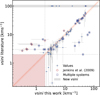 |
Fig. 6 v sin i values obtained in this work using the oversampled convolution method compared with literature measurements. Newly determined v sin i values not previously available are shown in the shaded area at v sin i (literature) = 100 km s−1. The solid line indicates the 1:1 relation, while the dashed lines correspond to a 10% deviation. Dashed grey lines and the shaded area mark the 2 km s−1 limit of CARMENES. Values inside this region are not plotted. |
 |
Fig. 7 Values of v sin i derived from the oversampled convolution method compared to veq. The linear |
![Mathematical equation: $\[1\text{:} \frac{4}{\pi}\]$](/articles/aa/full_html/2026/05/aa59177-26/aa59177-26-eq14.png)
![Mathematical equation: $\[1\text{:} \frac{1}{2}\]$](/articles/aa/full_html/2026/05/aa59177-26/aa59177-26-eq15.png)
Targets with unreliable v sin i values.
 |
Fig. 8 Histogram of the normalised difference between the v sin i value (> 2 km s−1) computed with oversampled convolution and the literature, excluding the outliers. The median is marked with a horizontal solid line. |
 |
Fig. 9 Top panel: comparison between v sin i computed with numerical integration and oversampled convolution. Dashed lines represent the 2 km s−1 limit and diagonal lines mark the 1:1 relation ±10%. Bottom panel: histogram of the normalised residuals with respect to the 1:1 relation for v sin i > 2 km s−1. Median value are represented by a vertical line. |
4.2 Numerical integration
The OC method is approximately 3.5 times faster than the NI approach, although the latter is expected to yield higher precision (see Sect. 3.4). Table 2 lists all v sin i values obtained with both methods, while Fig. 9 compares their results, which show excellent agreement. The histogram of the normalised residuals displays a median difference of only 0.1%, which is smaller than the offsets predicted from synthetic data in Sect. 3.4, where differences of about 1–2% were found for slow and intermediate rotators, and up to 5–10% for the fastest rotators (see Fig. 5).
Overall, values below and above 2 km s−1 are fully consistent between methods. The substantial increase in computational time relative to the modest gain in precision does not justify using NI instead of OC, particularly for statistical studies or slow-to-moderate rotators (v sin i < 20 km s−1). As discussed in Sect. 3.4, the improvement from NI only becomes noticeable for faster rotators (30–50 km s−1) and hotter stars (Teff = 4000 K). However, this effect remains minor for the CARMENES sample, yielding a similar median error to the OC method of 6.5%.
5 Conclusions
We present a novel method to determine the projected rotational velocity (v sin i) of stars from CARMENES-VIS spectra. This approach upgrades the serval pipeline by (i) adopting an order-dependent rotational broadening kernel that accounts for wavelength- and temperature-dependent stellar limb darkening, and (ii) performing spectral oversampling prior to convolution with the template spectrum. The effectiveness of these improvements has been tested using both synthetic and real datasets.
By applying this method, we derived a homogeneous catalogue of v sin i measurements for 392 M dwarfs observed with CARMENES-VIS. Our results show overall good agreement with previously published values, while achieving a substantially higher precision. The median relative uncertainty of our measurements is 6.8%, compared to 15.4% for literature values. Additionally, we report 36 new v sin i measurements that were not previously available. This catalogue provides a robust and homogeneous reference for studies of stellar rotation in low-mass stars and will be particularly valuable for the characterisation of M-dwarf planetary systems, including applications to age estimates, radial-velocity surveys, and spin–orbit investigations.
Data availability
Our pipeline, data, and results are available in a GitHub repository at https://github.com/rvarasg/vsini-limb-darkening. The full Table 2 is available at the CDS via https://cdsarc.cds.unistra.fr/viz-bin/cat/J/A+A/709/A244. The CARMENES DR1 dataset, which includes most of the spectra used in this work, is publicly available at https://carmenes.cab.inta-csic.es.
Acknowledgements
CARMENES is an instrument at the Centro Astronómico Hispano en Andalucía (CAHA) at Calar Alto (Almería, Spain), operated jointly by the Junta de Andalucía and the Instituto de Astrofísica de Andalucía (CSIC). Funding for CARMENES has been provided by the Max-Planck-Institut für Astronomie (MPIA), Consejo Superior de Investigaciones Científicas (CSIC), European Regional Development Fund (ERDF), Ministerio de Ciencia, Innovación y Universidades (MICIU), Deutsche Forschungsgemeinschaft (DFG), and the members of the CARMENES Consortium (https://carmenes.caha.es). This publication was based on observations collected under the CARMENES Legacy-Plus project. The authors wish to express their sincere thanks to all members of the Calar Alto staff for their expert support of the instrument and telescope operation. We used data from the CARMENES data archive at CAB (CSIC-INTA). We acknowledge financial support from the Agencia Estatal de Investigación (AEI/10.13039/501100011033) of the MICIU and the ERDF “A way of making Europe” through projects PID2022-137241-NBC4[1:4], PID2021- 125627OB-C3[1:2], PID2019-109522GB-C52, RYC2022-037854-I, and RYC2021-031640-I (2023AT003), and from the Centre of Excellence “Severo Ochoa” and “María de Maeztu” awards to the Instituto de Astrofísica de Andalucía (CEX2021-001131-S) and Institut de Ciències de l’Espai (CEX2020-001058-M). We also acknowledge financial support from the project AST22_00001_8 of the Junta de Andalucía and the Ministerio de Ciencia, Innovación y Universidades funded by the NextGenerationEU and the Plan de Recuperación, Transformación y Resiliencia.
References
- Barnes, J. R., Jenkins, J. S., Jones, H. R. A., et al. 2014, MNRAS, 439, 3094 [NASA ADS] [CrossRef] [Google Scholar]
- Baroch, D., Morales, J. C., Ribas, I., et al. 2020, A&A, 641, A69 [EDP Sciences] [Google Scholar]
- Bischoff, R., Mugrauer, M., Torres, G., et al. 2020, Astron. Nachr., 341, 908 [NASA ADS] [CrossRef] [Google Scholar]
- Bonfils, X., Delfosse, X., Udry, S., et al. 2013, A&A, 549, A109 [NASA ADS] [CrossRef] [EDP Sciences] [Google Scholar]
- Browning, M. K., Basri, G., Marcy, G. W., West, A. A., & Zhang, J. 2010, AJ, 139, 504 [NASA ADS] [CrossRef] [Google Scholar]
- Caballero, J. A., Guàrdia, J., López del Fresno, M., et al. 2016, SPIE Conf. Ser., 9910, 99100E [Google Scholar]
- Caballero, J. A., Cortés-Contreras, M., Alonso-Floriano, F. J., et al. 2017, in Highlights on Spanish Astrophysics IX, eds. S. Arribas, A. Alonso-Herrero, F. Figueras, C. Hernández-Monteagudo, A. Sánchez-Lavega, & S. Pérez-Hoyos, 496 [Google Scholar]
- Canocchi, G., Morello, G., Lind, K., et al. 2024, A&A, 692, A43 [NASA ADS] [CrossRef] [EDP Sciences] [Google Scholar]
- Carvalho, A., & Johns-Krull, C. M. 2023, RNAAS, 7, 91 [NASA ADS] [Google Scholar]
- Cifuentes, C., Caballero, J. A., Cortés-Contreras, M., et al. 2020, A&A, 642, A115 [NASA ADS] [CrossRef] [EDP Sciences] [Google Scholar]
- Cifuentes, C., Caballero, J. A., González-Payo, J., et al. 2025, A&A, 693, A228 [NASA ADS] [CrossRef] [EDP Sciences] [Google Scholar]
- Claret, A. 2000, A&A, 363, 1081 [NASA ADS] [Google Scholar]
- Claret, A., Hauschildt, P. H., & Torres, G. 2025, A&A, 699, A97 [NASA ADS] [CrossRef] [EDP Sciences] [Google Scholar]
- Cortés-Contreras, M., Caballero, J. A., Montes, D., et al. 2024, A&A, 692, A206 [NASA ADS] [CrossRef] [EDP Sciences] [Google Scholar]
- Delfosse, X., Forveille, T., Perrier, C., & Mayor, M. 1998, A&A, 331, 581 [NASA ADS] [Google Scholar]
- Diaz-Cordoves, J., & Gimenez, A. 1992, A&A, 259, 227 [Google Scholar]
- Díez Alonso, E., Caballero, J. A., Montes, D., et al. 2019, A&A, 621, A126 [NASA ADS] [CrossRef] [EDP Sciences] [Google Scholar]
- Fuhrmeister, B., Czesla, S., Schmitt, J. H. M. M., et al. 2018, A&A, 615, A14 [NASA ADS] [CrossRef] [EDP Sciences] [Google Scholar]
- Fuhrmeister, B., Czesla, S., Perdelwitz, V., et al. 2023, A&A, 670, A71 [NASA ADS] [CrossRef] [EDP Sciences] [Google Scholar]
- Gray, D. F. 2005, The Observation and Analysis of Stellar Photospheres, 3rd edn. (Cambridge University Press) [Google Scholar]
- Hauschildt, P. H., Barman, T., Baron, E., Aufdenberg, J. P., & Schweitzer, A. 2025, A&A, 698, A47 [NASA ADS] [CrossRef] [EDP Sciences] [Google Scholar]
- Henry, T. J., & Jao, W.-C. 2024, ARA&A, 62, 593 [Google Scholar]
- Henry, T. J., Jao, W.-C., Subasavage, J. P., et al. 2006, AJ, 132, 2360 [Google Scholar]
- Henry, T. J., Jao, W.-C., Winters, J. G., et al. 2018, AJ, 155, 265 [NASA ADS] [CrossRef] [Google Scholar]
- Hestroffer, D. 1997, A&A, 327, 199 [NASA ADS] [Google Scholar]
- Howarth, I. D. 2011, MNRAS, 418, 1165 [NASA ADS] [CrossRef] [Google Scholar]
- Jeffers, S. V., Schöfer, P., Lamert, A., et al. 2018, A&A, 614, A76 [NASA ADS] [CrossRef] [EDP Sciences] [Google Scholar]
- Jeffers, S. V., Barnes, J. R., Schöfer, P., et al. 2022, A&A, 663, A27 [NASA ADS] [CrossRef] [EDP Sciences] [Google Scholar]
- Jenkins, J. S., Ramsey, L. W., Jones, H. R. A., et al. 2009, ApJ, 704, 975 [Google Scholar]
- Kopal, Z. 1950, Harvard College Observ. Circ., 454, 1 [Google Scholar]
- Marfil, E., Tabernero, H. M., Montes, D., et al. 2021, A&A, 656, A162 [NASA ADS] [CrossRef] [EDP Sciences] [Google Scholar]
- Mas-Buitrago, P., González-Marcos, A., Solano, E., et al. 2024, A&A, 687, A205 [NASA ADS] [CrossRef] [EDP Sciences] [Google Scholar]
- Milne, E. A. 1921, MNRAS, 81, 361 [Google Scholar]
- Morales, J. C., Ribas, I., Jordi, C., et al. 2009, ApJ, 691, 1400 [NASA ADS] [CrossRef] [Google Scholar]
- Morello, G., Tsiaras, A., Howarth, I. D., & Homeier, D. 2017, AJ, 154, 111 [NASA ADS] [CrossRef] [Google Scholar]
- Morello, G., Claret, A., Martin-Lagarde, M., et al. 2020a, J. Open Source Softw., 5, 1834 [Google Scholar]
- Morello, G., Claret, A., Martin-Lagarde, M., et al. 2020b, AJ, 159, 75 [Google Scholar]
- Morello, G., Casasayas-Barris, N., Orell-Miquel, J., et al. 2022, A&A, 657, A97 [NASA ADS] [CrossRef] [EDP Sciences] [Google Scholar]
- Newton, E. R., Irwin, J., Charbonneau, D., et al. 2016, ApJ, 821, 93 [Google Scholar]
- Palle, E., Nortmann, L., Casasayas-Barris, N., et al. 2020, A&A, 638, A61 [EDP Sciences] [Google Scholar]
- Passegger, V. M., Bello-García, A., Ordieres-Meré, J., et al. 2020, A&A, 642, A22 [NASA ADS] [CrossRef] [EDP Sciences] [Google Scholar]
- Poveda, A., Allen, C., Costero, R., Echevarría, J., & Hernández-Alcántara, A. 2009, ApJ, 706, 343 [Google Scholar]
- Quirrenbach, A., Amado, P. J., Caballero, J. A., et al. 2014, SPIE Conf. Ser., 9147, 91471F [Google Scholar]
- Quirrenbach, A., Amado, P. J., Ribas, I., et al. 2018, SPIE Conf. Ser., 10702, 107020W [Google Scholar]
- Reiners, A., Joshi, N., & Goldman, B. 2012, AJ, 143, 93 [Google Scholar]
- Reiners, A., Zechmeister, M., Caballero, J. A., et al. 2018, A&A, 612, A49 [NASA ADS] [CrossRef] [EDP Sciences] [Google Scholar]
- Reiners, A., Shulyak, D., Käpylä, P. J., et al. 2022, A&A, 662, A41 [NASA ADS] [CrossRef] [EDP Sciences] [Google Scholar]
- Ribas, I., Reiners, A., Zechmeister, M., et al. 2023, A&A, 670, A139 [NASA ADS] [CrossRef] [EDP Sciences] [Google Scholar]
- Ruh, H. L., Zechmeister, M., Reiners, A., et al. 2024, A&A, 692, A138 [NASA ADS] [CrossRef] [EDP Sciences] [Google Scholar]
- Sabotta, S., Schlecker, M., Chaturvedi, P., et al. 2021, A&A, 653, A114 [NASA ADS] [CrossRef] [EDP Sciences] [Google Scholar]
- Schöfer, P., Jeffers, S. V., Reiners, A., et al. 2019, A&A, 623, A44 [Google Scholar]
- Shan, Y., Revilla, D., Skrzypinski, S. L., et al. 2024, A&A, 684, A9 [NASA ADS] [CrossRef] [EDP Sciences] [Google Scholar]
- Soto, M. G., Anglada-Escudé, G., Dreizler, S., et al. 2021, A&A, 649, A144 [NASA ADS] [CrossRef] [EDP Sciences] [Google Scholar]
- Suárez Mascareño, A., Rebolo, R., González Hernández, J. I., & Esposito, M. 2015, MNRAS, 452, 2745 [Google Scholar]
- Zechmeister, M., Reiners, A., Amado, P. J., et al. 2018, A&A, 609, A12 [NASA ADS] [CrossRef] [EDP Sciences] [Google Scholar]
Appendix A v sin i using near-infrared spectra
We analysed v sin i using both CARMENES-NIR and VIS spectra for the coldest stars in the sample (16 objects). This selection is motivated by their higher near-infrared S/N relative to hotter stars, comparable to the VIS S/N (Reiners et al. 2018). J07403-174 and J02530+168 were used as templates (Table 1), and their v sin i values are not computed here. For this preliminary analysis, we did not apply oversampling nor include limb-darkening.
Figure A.1 presents the comparison of v sin i derived from NIR and VIS spectra for this subsample. Most measurements are consistent between the two datasets, with a few cases close to or below the 2 km s−1 limit. A more detailed analysis, analogous to that performed for the VIS data in this study, is required to fully characterise the small remaining differences between the NIR and VIS results.
 |
Fig. A.1 Comparison of v sin i derived from CARMENES-VIS and NIR spectra for M dwarfs later than M6.0 V. No oversampling or limb-darkening was applied. Lines indicate the 1:1 relation (± 10%) and the 2 km s−1 limit. |
Appendix B Rotation kernel with limb-darkening
Following Gray (2005), the disc-integrated spectrum of a rigidly rotating, spherical star can be written as a convolution:
![Mathematical equation: $\[F(v)=\int_{-v ~\sin~ i}^{+v ~\sin~ i} S(v-v^{\prime}) \tilde{K}(v^{\prime}) ~d v^{\prime}\]$](/articles/aa/full_html/2026/05/aa59177-26/aa59177-26-eq16.png) (B.1)
(B.1)
where S(v) is the intrinsic, non-rotating stellar spectrum, and
![Mathematical equation: $\[v=c \frac{\lambda-\lambda_{\mathrm{ref}}}{\lambda_{\mathrm{ref}}}\]$](/articles/aa/full_html/2026/05/aa59177-26/aa59177-26-eq17.png) (B.2)
(B.2)
is the Doppler velocity relative to a reference wavelength. The kernel ![Mathematical equation: $\[\tilde{K}(v^{\prime})\]$](/articles/aa/full_html/2026/05/aa59177-26/aa59177-26-eq18.png) represents the relative contribution of all surface elements sharing the same projected line-of-sight velocity v′. Choosing the x-axis along the projected stellar equator, the line-of-sight velocity of a surface element is
represents the relative contribution of all surface elements sharing the same projected line-of-sight velocity v′. Choosing the x-axis along the projected stellar equator, the line-of-sight velocity of a surface element is
![Mathematical equation: $\[v^{\prime}(x)=(v ~\sin~ i) x, \quad-1 \leq x \leq 1,\]$](/articles/aa/full_html/2026/05/aa59177-26/aa59177-26-eq19.png) (B.3)
(B.3)
in normalised Cartesian coordinates on the projected stellar disc. Each value of v′ therefore corresponds to a chord across the stellar disc perpendicular to the projected equator. The unnormalised kernel is obtained by integrating the surface intensity along these chords,
![Mathematical equation: $\[K(x)=\int_{-a}^a I(x, y) ~d y, \quad a=\sqrt{1-x^2}.\]$](/articles/aa/full_html/2026/05/aa59177-26/aa59177-26-eq20.png) (B.4)
(B.4)
We assume radial limb-darkening, so that I(x, y) = I(μ) with ![Mathematical equation: $\[\mu=\sqrt{1-x^{2}-y^{2}}\]$](/articles/aa/full_html/2026/05/aa59177-26/aa59177-26-eq21.png) . Most commonly used limb-darkening laws can be written as linear combinations of powers of μ:
. Most commonly used limb-darkening laws can be written as linear combinations of powers of μ:
![Mathematical equation: $\[I(\mu)=\sum_\gamma c_\gamma \mu^\gamma.\]$](/articles/aa/full_html/2026/05/aa59177-26/aa59177-26-eq22.png) (B.5)
(B.5)
Replacing the above intensity profile into Eq. (B.4), the kernel becomes
![Mathematical equation: $\[K(x)=\sum_\gamma c_\gamma \int_{-a}^a\left(a^2-y^2\right)^{\frac{\gamma}{2}} ~d y, \quad a=\sqrt{1-x^2}.\]$](/articles/aa/full_html/2026/05/aa59177-26/aa59177-26-eq23.png) (B.6)
(B.6)
Applying the substitution y = a cos t,
![Mathematical equation: $\[K(x)=\sum_\gamma c_\gamma a^{\gamma+1} \int_0^\pi(\sin~ t)^{\gamma+1} d t, \quad a=\sqrt{1-x^2}.\]$](/articles/aa/full_html/2026/05/aa59177-26/aa59177-26-eq24.png) (B.7)
(B.7)
In absence of limb-darkening, there is only one term with γ = 0 (c0 = 1), so
![Mathematical equation: $\[K_{\mathrm{unif}}(x)=2 ~\sqrt{1-x^2}.\]$](/articles/aa/full_html/2026/05/aa59177-26/aa59177-26-eq25.png) (B.8)
(B.8)
The linear limb-darkening law coincides with Eq. (B.5) for c0 = 1 − u and c1 = u. The corresponding un-normalised kernel is
![Mathematical equation: $\[K_{\operatorname{lin}}(x)=2(1-u) ~\sqrt{1-x^2}+\frac{\pi}{2} u(1-x^2).\]$](/articles/aa/full_html/2026/05/aa59177-26/aa59177-26-eq26.png) (B.9)
(B.9)
The kernel for the quadratic law is obtained with c0 = 1 − u1 − u2, c1 = u1 + 2u2 and c2 = −u2:
![Mathematical equation: $\[K_{\text {quad }}(x)=2(1-u_1-u_2) ~\sqrt{1-x^2}+\frac{\pi}{2}(u_1+2 u_2)(1-x^2)-\frac{4}{3} u_2(1-x^2)^{\frac{3}{2}}.\]$](/articles/aa/full_html/2026/05/aa59177-26/aa59177-26-eq27.png) (B.10)
(B.10)
The integrals for non-integer γ exponents do not admit a closed-form analytical solution. They can, however, be expressed in terms of the Γ function:
![Mathematical equation: $\[\int_0^\pi(\sin~ t)^{\gamma+1} ~d t=\pi \frac{\Gamma\left(\frac{\gamma+2}{2}\right)}{\Gamma\left(\frac{\gamma+3}{2}\right)}, \quad \gamma>-2.\]$](/articles/aa/full_html/2026/05/aa59177-26/aa59177-26-eq28.png) (B.11)
(B.11)
By combining Eqs. (B.6) and (B.11), the broadening kernel can be computed for other limb-darkening laws, including the square-root, power-2, and four-coefficient prescriptions.
Appendix C Numerical aspects of the rotation kernel
Figure C.1 shows the resulting normalised kernel in Eq. (8) for selected values of the limb-darkening coefficient u. The kernel transitions from a semi-circular profile for u = 0 to an increasingly parabolic shape as u → 1. We derived the effective width of each kernel, σu, where ![Mathematical equation: $\[\sigma_{u}^{2}\]$](/articles/aa/full_html/2026/05/aa59177-26/aa59177-26-eq29.png) corresponds to the kernel variance including limb-darkening. The ratio σu/σ0 is a measure of the underestimation of v sin i when limb-darkening is neglected. For instance, u = 0.6 leads to an underestimation of approximately 6%. As illustrated by the narrower kernel at higher u, neglecting limb-darkening biases the recovered v sin i toward lower values.
corresponds to the kernel variance including limb-darkening. The ratio σu/σ0 is a measure of the underestimation of v sin i when limb-darkening is neglected. For instance, u = 0.6 leads to an underestimation of approximately 6%. As illustrated by the narrower kernel at higher u, neglecting limb-darkening biases the recovered v sin i toward lower values.
 |
Fig. C.1 Rotational broadening kernel for different limb-darkening coefficients u. Circular markers correspond to the effective width of each kernel. |
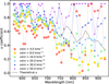 |
Fig. C.2 Limb-darkening u coefficient as a function of wavelength, when fitting simultaneously with v sin i. |
We attempted to simultaneously fit v sin i and the limb-darkening coefficient u using the oversampled convolution method, but found notable inconsistencies. The fitted u values vary systematically with the target’s v sin i (see Fig. C.2), and for higher rotational velocities and Teff, where the method becomes less reliable (Sect. 3.4), u tends to converge toward 1 across all spectral orders, attempting to compensate for discrepancies between the input and recovered v sin i. Furthermore, the fitted coefficients show poor agreement with the theoretical predictions.
We examined whether the limitations of the method could arise from an overly simplified treatment of limb-darkening. In the context of exoplanetary transit studies, the most commonly employed laws are linear (Milne 1921), quadratic (Kopal 1950), square-root (Diaz-Cordoves & Gimenez 1992), four-coefficient (Claret 2000), and power-2 (Hestroffer 1997). Figure C.3 shows the differences between the fitted v sin i values obtained as a function of the target’s v sin i, for 4000 K. The discrepancies among the non-linear models are minimal, remaining below 0.5% even in the most extreme cases when compared to the linear law.
 |
Fig. C.3 Normalized difference between input and fitted v sin i as a function of the input v sin i for different limb-darkening laws. |
Appendix D Oversampling and limb-darkening impact during convolution
Table D.1 presents the results obtained using regular convolution without limb-darkening (RCWLD) and oversampled convolution with linear limb-darkening (OCLLD) for all combinations of v sin i and Teff in our spectral sample. In general, the more sophisticated approach yields values closer to the target v sin i and with smaller uncertainties. The simplest method systematically underestimates the rotational broadening of the target spectrum and, in most cases, does not agree with the target value within the errors.
Derived v sin i values for all the Teff and target v sin i combinations, using regular convolution without limb-darkening (RCWLD) and oversampled convolution with linear limb-darkening (OCLLD).
Appendix E Comparison with other works
We also compared our catalogue with the results of Passegger et al. (2020) and Mas-Buitrago et al. (2024, see our Fig. E.1), who derived the projected rotational velocities of CARMENES targets using deep-learning methods. Their v sin i values are typically larger, particularly for slow rotators. For v sin i above 10 km s−1, the differences decrease. Both studies also report systematically higher v sin i values than those derived by Reiners et al. (2018). Our results lie between these estimates, but are closer to those of Reiners et al. (2018) and Reiners et al. (2022).
 |
Fig. E.1 Comparison of our v sin i values with the results from Passegger et al. (2020) and Mas-Buitrago et al. (2024) |
 |
Fig. E.2 rms of the residuals between target spectrum and template rotationally broadened using both v sin i from this work and Mas-Buitrago et al. (2024). |
For all targets in common with Mas-Buitrago et al. (2024), we compared the stellar spectrum with the corresponding template (see Table 1) rotationally broadened using both sets of v sin i values. The rms of the residuals is shown in Fig. E.2. In general, our v sin i measurements yield smaller rms values, particularly for slow rotators. This indicates that our results reproduce the observed broadening of the spectral lines in the CARMENES VIS spectra more accurately.
Appendix F Spectrum and v sin i of J14155+046
Jenkins et al. (2009) reported a projected rotational velocity of v sin i = 6.8 km s−1 for J14155+046. In our analysis, we obtained a value below 2 km s−1, which corresponds to the lower limit of our method. Comparing the spectrum of J14155+046 with that of J03133+047, a reference star in our sample with v sin i < 2 km s−1, we find a better match than when broadening the spectrum of J03133+047 to higher velocities, as the rms of the residuals halve (see Fig. F.1).
 |
Fig. F.1 Top: Chunk of the CARMENES-VIS co-added spectrum of J14155+046 compared to the spectrum of J03133+047, without and with 6.8 km s−1 rotational broadening (Jenkins et al. 2009). Bottom: Residuals with respect to J14155+046. |
All Tables
Stars used as templates for computing v sin i depending on spectral type (Schöfer et al. 2019).
Catalogue of v sin i values for 392 M-dwarf stars of the CARMENES sample using VIS spectra a.
Derived v sin i values for all the Teff and target v sin i combinations, using regular convolution without limb-darkening (RCWLD) and oversampled convolution with linear limb-darkening (OCLLD).
All Figures
|
Fig. 1 χ2 minimization between reference and target synthetic spectra as a function of v sin i for three spectral orders, computed without limb-darkening correction. The spectra correspond to Teff = 3000 K, with a target value of v sin i = 8 km s−1 (vertical line). |
| In the text | |
|
Fig. 2 Top: χ2 minimization as a function of v sin i for different oversampling factors. Bottom: residuals relative to the best-fit solution (oversampling factor = 9). The convolution kernel does not include any limb-darkening effect. The vertical line marks the target value v sin i = 8 km s−1, obtained from synthetic spectra with Teff = 3000 K. |
| In the text | |
|
Fig. 3 Best-fitting v sin i values as a function of wavelength for different oversampling factors, obtained without accounting for limb-darkening in the convolution process. Horizontal lines correspond to the median values. The spectra correspond to Teff = 3000 K and a target value of v sin i = 8 km s−1. |
| In the text | |
|
Fig. 4 Best-fitting v sin i values as a function of wavelength, obtained with and without accounting for limb darkening during the convolution. Horizontal solid lines indicate the median values, and the shaded regions represent the standard deviations. The dashed line marks the target value v sin i = 8 km s−1 for spectra with Teff = 3000 K. |
| In the text | |
|
Fig. 5 Normalised difference between input and fitted v sin i as a function of input v sin i and a spectrum’s Teff, for oversampled convolution (top panel) and numerical integration (bottom panel). |
| In the text | |
|
Fig. 6 v sin i values obtained in this work using the oversampled convolution method compared with literature measurements. Newly determined v sin i values not previously available are shown in the shaded area at v sin i (literature) = 100 km s−1. The solid line indicates the 1:1 relation, while the dashed lines correspond to a 10% deviation. Dashed grey lines and the shaded area mark the 2 km s−1 limit of CARMENES. Values inside this region are not plotted. |
| In the text | |
|
Fig. 7 Values of v sin i derived from the oversampled convolution method compared to veq. The linear |
| In the text | |
|
Fig. 8 Histogram of the normalised difference between the v sin i value (> 2 km s−1) computed with oversampled convolution and the literature, excluding the outliers. The median is marked with a horizontal solid line. |
| In the text | |
|
Fig. 9 Top panel: comparison between v sin i computed with numerical integration and oversampled convolution. Dashed lines represent the 2 km s−1 limit and diagonal lines mark the 1:1 relation ±10%. Bottom panel: histogram of the normalised residuals with respect to the 1:1 relation for v sin i > 2 km s−1. Median value are represented by a vertical line. |
| In the text | |
|
Fig. A.1 Comparison of v sin i derived from CARMENES-VIS and NIR spectra for M dwarfs later than M6.0 V. No oversampling or limb-darkening was applied. Lines indicate the 1:1 relation (± 10%) and the 2 km s−1 limit. |
| In the text | |
|
Fig. C.1 Rotational broadening kernel for different limb-darkening coefficients u. Circular markers correspond to the effective width of each kernel. |
| In the text | |
|
Fig. C.2 Limb-darkening u coefficient as a function of wavelength, when fitting simultaneously with v sin i. |
| In the text | |
|
Fig. C.3 Normalized difference between input and fitted v sin i as a function of the input v sin i for different limb-darkening laws. |
| In the text | |
|
Fig. E.1 Comparison of our v sin i values with the results from Passegger et al. (2020) and Mas-Buitrago et al. (2024) |
| In the text | |
|
Fig. E.2 rms of the residuals between target spectrum and template rotationally broadened using both v sin i from this work and Mas-Buitrago et al. (2024). |
| In the text | |
|
Fig. F.1 Top: Chunk of the CARMENES-VIS co-added spectrum of J14155+046 compared to the spectrum of J03133+047, without and with 6.8 km s−1 rotational broadening (Jenkins et al. 2009). Bottom: Residuals with respect to J14155+046. |
| In the text | |
Current usage metrics show cumulative count of Article Views (full-text article views including HTML views, PDF and ePub downloads, according to the available data) and Abstracts Views on Vision4Press platform.
Data correspond to usage on the plateform after 2015. The current usage metrics is available 48-96 hours after online publication and is updated daily on week days.
Initial download of the metrics may take a while.