| Issue |
A&A
Volume 710, June 2026
|
|
|---|---|---|
| Article Number | A43 | |
| Number of page(s) | 16 | |
| Section | Stellar structure and evolution | |
| DOI | https://doi.org/10.1051/0004-6361/202659539 | |
| Published online | 29 May 2026 | |
The NuSTAR view of ultra-compact X-ray binaries
1
European Space Agency (ESA), European Space Astronomy Center (ESAC), Camino Bajo del Castillo s/n, 28692 Villafranca del Castillo, Madrid, Spain
2
Instituto de Astrofísica de Canarias, E-38205 La Laguna, Tenerife, Spain
3
Departamento de Astrofísica, Universidad de La Laguna, E-38206 La Laguna, Tenerife, Spain
★ Corresponding author: This email address is being protected from spambots. You need JavaScript enabled to view it.
Received:
20
February
2026
Accepted:
10
April
2026
Abstract
Ultra-compact X-ray binaries (UCXBs) are a subclass of low-mass X-ray binaries (LMXBs) characterised by tight orbits and hydrogen-poor donor stars. We present a spectral and timing study in the hard X-ray band of 11 of the 20 confirmed UCXBs, based on 37 archival NuSTAR observations. Using both X-ray colours and fractional root mean square values, we show that our sample spans the hard, soft, and intermediate X-ray states. Subsequently, we performed an X-ray spectral analysis using, when data allowed, the three-component model – an approach increasingly adopted for neutron star LMXBs. This work represents the largest LMXB sample analysed to date with this methodology. We focus on the properties of the X-ray continuum and report typical values for each X-ray state. Overall, UCXBs exhibit similar spectral properties to their longer-period counterparts, suggesting no major differences in the innermost regions of X-ray binaries regardless of disc size or chemical composition. A possible exception is found in the soft-state sample, which shows Comptonisation fractions higher than those typically observed in regular LMXBs, although the statistics remain limited. Finally, we discuss the case of the slow X-ray pulsar 4U 1626–67, where we report the discovery of a very cold hard state with an electron temperature of ∼6 keV – comparable to those usually observed in soft states of neutron-star LMXBs.
Key words: binaries: general / stars: low-mass / novae / cataclysmic variables
ESA Research Fellow.
© The Authors 2026
 Open Access article, published by EDP Sciences, under the terms of the Creative Commons Attribution License (https://creativecommons.org/licenses/by/4.0), which permits unrestricted use, distribution, and reproduction in any medium, provided the original work is properly cited.
This article is published in open access under the Subscribe to Open model. This email address is being protected from spambots. You need JavaScript enabled to view it. to support open access publication.
1. Introduction
Ultra-compact X-ray binaries (UCXBs) are a group of low-mass X-ray binaries (LMXBs) with shorter orbital periods (Porb < 60–80 min) than those of the ‘classical’ LMXBs (Porb∼ hours to tens of days). The tight orbits of these systems imply that the compact object, either a neutron star (NS) or a black hole (BH), is accreting via Roche-lobe overflow from a hydrogen-poor companion (Rappaport et al. 1982). These systems play a crucial role in different aspects of astrophysics: i) UCXBs are strong, persistent gravitational wave sources for future missions that are sensitive in the low-frequency regime (e.g., Chen et al. 2021); ii) they provide important tests of binary evolution theories; iii) they enable investigations into the accretion processes under hydrogen-poor conditions (e.g., Nelemans et al. 2009).
At the moment of writing (April 2026), 20 LMXBs have been proven to be UCXBs, that is, with confirmed Porb measurements, as reported by Armas Padilla et al. (2023), who built the first comprehensive catalogue of confirmed and candidate UCXBs (UltraCompCAT1). Pinpointing UCXBs by measuring the Porb can be challenging, and thus indirect methods of identifying candidates are often relied on. In these systems, the accretion disc is small, and thus the disc region responsible for the X-ray to optical reprocessing is also small. Therefore, UCXBs show lower optical-to-X-ray flux ratios than ‘classical’ LMXBs at the same X-ray flux (van Paradijs & McClintock 1994). Moreover, persistent LMXBs with low X-ray luminosity (LX, pers < 1036 erg s−1) can hide UCXBs since small discs can be entirely ionised at lower accretion rates (Lasota 2001; in’t Zand et al. 2007). Additional diagnostics are based on spectral data, such as the absence of hydrogen lines in the optical spectra (e.g., Stoop et al. 2021) and the presence of X-ray features due to overabundances in the accreted material (e.g., Armas Padilla & López-Navas 2019).
As is the case for LMXBs, UCXBs can be persistent sources, always active, or transient, exhibiting outbursts with recurrence times from months to years (see e.g., for a review Bahramian & Degenaar 2023). During an outburst, two main accretion states can be identified, namely hard and soft states. A hard state is observed at the beginning and at the end of an outburst. The X-ray spectrum roughly follows a power-law shape with cut-off energies of approximately tens of keV for NS systems and up to roughly hundreds of keV for BH sources (Burke et al. 2017; Banerjee et al. 2020). This component arises from a geometrically thick, optically thin inflow, the so-called corona, which Comptonises softer X-ray photons coming from the accretion disc and/or boundary layer (for NS systems). Contrastingly, during the soft state, the X-ray emission is dominated by the optically thick, geometrically thin accretion disc that moves inward and becomes hotter, cooling down the corona. In addition to these two states, intermediate states can be found when the source transitions from the hard to the soft state and vice versa, with the soft-to-hard transition occurring at lower luminosities than the hard-to-soft one.
Several studies have been performed for each of the UCXBs, while global investigations of this class of LMXBs remain very scarce. For instance, Fiocchi et al. (2008) carried out a systematic spectral analysis of a small sample of UCXBs using INTEGRAL combined with BeppoSAX and Swift data whenever possible. They found that these systems spend most of the time in hard states and that all spectra were well described by a two-component model consisting of a disk-blackbody and Comptonised emission. Koliopanos et al. (2021) primarily employed XMM–Newton data of 14 confirmed and two then candidate UCXBs to constrain the chemical composition of their accretion disc through a homogeneous spectral study focusing on the presence of the iron Kα emission line. Recently, Dage et al. (2025) presented a global study of the radio counterparts of UCXBs, reporting no strong evidence of a correlation between the radio luminosity and the orbital period. Moreover, they studied the properties of the globular clusters hosting UCXBs with respect to a sample of globular clusters where no known UCXBs reside, noting that the former group has much higher encounter rates than the latter.
In this work, we present for the first time a self-consistent analysis of the X-ray spectral properties and variability of the confirmed UCXBs as a population while making use of publicly available2 observations of the Nuclear Spectroscopic Telescope Array (NuSTAR; Harrison et al. 2013). This sums up to 37 pointings for 11 sources for a total on-source exposure time of 1.2 Ms. In Section 2, we summarise the X-ray data analysis procedure. We then describe the details and results of the analysis in Section 3. Finally, implications are discussed in Section 4.
2. Observations and data reduction
Launched in 2012, NuSTAR is the first observatory focusing on hard X-rays. It consists of two co-aligned optics focused onto two focal planes, referred to as FPMA and FPMB, observing the sky in the energy range from 3 to 79 keV. Its effective area peaks at ∼900 cm−2 around 10 keV when combining the two modules. NuSTAR achieves an energy resolution of 400 eV at 10 keV and an angular resolution of 18″ full width at half maximum.
We found 37 NuSTAR observations for 11 systems in the HEASARC Data Archive. We report a log of the observations included in this work in Appendix A and detail the properties of the 11 UCXBs in Table 1, as taken from the catalog UltraCompCAT (Armas Padilla et al. 2023, and references therein).
Main properties of the UCXBs included in this work. The sources are sorted by increasing orbital period.
Data reduction was performed using the NuSTAR Data Analysis Software (NUSTARDAS), which is part of the HEASOft package (v.6.32), and the most recent calibration files. We processed the raw data with the tool NUPIPELINE to generate cleaned event lists and filtered out passages of the satellite through the South Atlantic Anomaly. We selected the source photons from a circular region with a typical radius of 100–120″, depending on the source brightness. Noteworthy exceptions are IGR J17494−3030 and 47 Tuc X−9. For the former, we adopted an 80-arcsec radius circle to maximise the source signal-to-noise ratio (it is the UCXB with the lowest net count rate in the 3–15 keV band, 0.072 ± 0.001 counts s−1). 47 Tuc X−9 is located in the core of the globular cluster 47 Tucanae. To minimise the contamination from other sources of the cluster core, we opted for a circle with a radius of 30″. In all cases, the background counts were accumulated within a region far from the target and of the same size as that adopted for the source. Swift J1756.9–2508 was not detected during the second available observation, which was carried out when the source returned to quiescence after its 2018 outburst (Sanna et al. 2018b; Li et al. 2021). Stray light contamination, which is unfocused light from bright sources outside the field of view of NuSTAR, is evident, and the source region is embedded in it. We derived an upper limit of ∼0.34 counts s−1 on the 3–15 keV source count rate, considering only the FPMA event file.
For each observation, we built the source light curve with different timing resolutions to check for the presence of type I X-ray bursts, and if detected, we applied intensity filters to the event lists. The source 4U 1916–053 shows periodic dips (Walter et al. 1982). Being interested in the persistent emission, we performed a time selection on the data. We created source and background spectra and the corresponding redistribution matrices and ancillary response files using the NUPRODUCTS pipeline. For 47 Tuc X−9, the two available observations were performed only one day apart. Therefore, we merged them to increase the source signal-to-noise ratio. This object is the principal source of X-rays in the cluster above 6 keV (Bahramian et al. 2017). Therefore, we limited our analysis to photons with energies higher than 6 keV, which is at odds with all the others sources where we considered energies higher than 3 keV.
3. Analysis and results
In the following, all uncertainties are quoted at 1σ confidence level unless specified otherwise.
3.1. Power density spectra and hardness
In order to study the variability of the source, we selected events in the 3–15 keV energy range, with the exception of 47 Tuc X−9 (6–15 keV). We built the Leahy normalised power density spectra (PDS) using the library Stingray (Huppenkothen et al. 2019) and performing the dead-time correction on each NuSTAR PDS by means of the Fourier amplitude difference technique (Bachetti & Huppenkothen 2018). For each observation, we averaged the PDS obtained from 50-s long segments with time bins of 5 ms. For each PDS, we computed the fractional root mean square (RMS) variability in the 0.1–64 Hz frequency range. Instead of subtracting the Poisson noise contribution, we fitted it with a constant component at high frequencies. For only two sources, 47 Tuc X–9 and IGR J17494–3030, the RMS value is not constrained, most likely due to the low statistics. Moreover, we derived the hardness as the ratio of the source count rates estimated from the FPMA event file between the 10–16 and 6–10 keV energy bands. We adopted these energy bands to reduce contamination from the interstellar absorption and the contribution from the soft thermal components. In this way, the hardness can be exploited as an independent tool to trace the Comptonisation fraction.
We favoured the frequency and energy ranges mentioned above for the RMS and hardness in order to be able to compare our results with those presented by Muñoz-Darias et al. (2014), who performed a systematic analysis of the X-ray colour and fast variability of 50 NS LMXBs monitored by the Rossi X-ray Timing Explorer (RXTE). We are aware that the RXTE energy band extended down to 2 keV. We took this information into account when comparing our findings.
3.2. Spectral analysis
The NuSTAR background-subtracted spectra were grouped using the optimal binning scheme of Kaastra & Bleeker (2016) by means of the ftool FTGROUPPHA. Spectral analysis was performed using XSPEC (version 12.13.1; Arnaud 1996) and the χ2 statistic. To describe the effects of the photoelectric absorption along the line of sight, we adopted the tbabs model with photoionisation cross-sections of Verner et al. (1996) and chemical abundances of Wilms et al. (2000). For each observation, we simultaneously fit the spectra for both FPMs, adding a renormalisation constant to account for cross-calibration uncertainties between the two telescopes (we froze it to one for FPMA). In every fit, we fixed the hydrogen column density NH to the value reported in Table 1. Once the best fit for the adopted model was found, the observed and unabsorbed fluxes were estimated with the convolution model cflux in the 0.8–30 keV energy band.
In the cases of 4U 1543–624, 4U 1626–67 (first epoch), and 4U 1820–303 (all epochs except the first two), the observations provided high-statistical-quality spectra, where systematic calibration uncertainties are important. Therefore, we added an energy independent systematic uncertainty of 0.5% to each spectral channel3.
3.2.1. Spectral models
For the thermal emission, we tested two models:
-
The blackbody model bbodyrad (BB), parametrised by its temperature kTBB and normalisation NBB, the latter being connected to the blackbody emitting radius through the formula RBB
 , with D10kpc as the distance of the source in units of 10 kpc. This model accounts for the NS surface and boundary layer emission.
 -
The multi-colour disc model diskbb for the accretion disc emission (DISC, e.g., Mitsuda et al. 1984), characterised by the temperature at the inner disc radius kTdisc and normalisation Ndisc, which can be translated into the inner disc radius, Rdisc, with the relation
where ξ is the correction factor for the inner torque-free boundary condition (Kubota et al. 1998), κ is the ratio of colour temperature to the effective temperature (Shimura & Takahara 1995), and i is the inclination of the system. We assumed ξ = 0.4 and κ = 1.7. For the inclination, we adopted a value of 43° for 4U 1820–303 derived from the modelling of the ultraviolet flux modulation of the system (Anderson et al. 1997). The presence of dips and lack of eclipses in the light curve of 4U 1916–053 constrained the inclination of the system to be i≲ 79° (Smale et al. 1988). Previous works (e.g., Boirin et al. 2004) assumed i = 70°, so we adopted the same value. The other sources in the sample do not show eclipses or dips, setting an upper limit of i ≲ 75° on the inclination angle (e.g., Degenaar et al. 2017; Sanna et al. 2017, 2018b), and we chose a representative value of 70°.
We applied the nthcomp model (NTHCOMP) to take into account the contribution of the Comptonisation corona (Zdziarski et al. 1996; Życki et al. 1999). The involved parameters are the power-law photon index, Γ; the electron temperature of the Comptonising medium, kTe; the seed photon temperature, kTseed; and the normalisation, Ncomp. The seed photons might come from the disc or the NS (boundary layer and/or surface). Therefore, when combining the nthcomp model with the BB and/or DISC components, we linked kTseed to kTBB or kTdisc and changed the seed photon shape parameter inp_type accordingly: 0 for BB or 1 for DISC shape.
When the Fe Kα emission line was observed, a simple Gaussian component (gauss in XSPEC) was included in the model, and its width was fixed to the values reported in the literature (4U 1543–624 being the exception with width free). We detected the Fe feature at all epochs for 4U 1543–624, 4U 0614+091, and IGR J17062–6143, while for 4U 1820–303 the spectral line was present in ten of the 11 observations. The second source with a variable presence of the iron line is 4U 1626–67. The feature is broad, with a central energy of ∼6.8 keV. D’Aì et al. (2017) suggested that the feature is a possible blending of two lines because the central energy lies between the energy of the Lyα transitions of the He-like (6.70 keV) and the H-like (6.97 keV) iron ions. This system is unique, as it is the only UCXB harbouring a slow-spinning (7.7 s) NS with a magnetic field of ∼(3–4) × 1012 G, as estimated from a resonant cyclotron scattering feature at ∼35–37 keV (Rappaport et al. 1977; Orlandini et al. 1998). We used the gabs component to model the resonant cyclotron scattering feature. We found no evidence of the iron emission line for 4U 1916–053. However, the spectrum showed two narrow absorption features at ∼8.14 keV and ∼6.77 keV, which might be the Fe XXVI Kβ and Fe XXV Kα absorption lines. We modelled them using the additive spectral component gauss with the width frozen at 20 eV (Gambino et al. 2019). In the spectra of the remaining sources (MAXI J0911–655, Swift J1756.9–2508, IGR J16597–3704, IGR J17494–3030 and 47 Tuc X–9), we did not detect any feature.
3.2.2. Spectral fits
At this stage of the study, we modelled the spectra regardless of the state of the source. To select the acceptable fits from a statistical point of view, we considered the null hypothesis probability (nhp), which represents the probability that the deviations between the data and the model are due to chance alone. In general, a model can be rejected when the nhp is smaller than 0.05 (see e.g., Armas Padilla et al. 2017; Armas Padilla & López-Navas 2019).
For each spectrum, we started by fitting it with the simplest model, meaning a one-component model such as a BB, DISC, or NTHCOMP. The number of required components was evaluated by means of an F-test: an additional component was included if it yielded an improvement in the fit of at least 3σ. When a second component was required, we combined the Comptonised component with a thermal one (i.e., DISC+NTHCOMP or BB+NTHCOMP). In the case of a three-component model, we employed the model DISC+BB+NTHCOMP with two possible solutions for the seed photon temperature: kTseed = kTdisc or kTseed = kTBB. Therefore, hereafter, we refer to these as the DISC and BB approaches, respectively. We note that for every spectrum, we tested both approaches. In the cases where the best fit is provided by a three-component model, uncertainties on the parameters have been computed in two steps, that is, by freezing the thermal components when estimating the error associated with the parameters of the NTHCOMP model and vice versa, given the degeneracy of the model.
Following the above-mentioned criteria (i.e., nhp and F-test), we found that for seven systems, the three-component model was the best-fit model at all epochs. For 4U 1543–624 (one spectrum), the F-test showed that the three-component model was significantly better than a two-component one. However, the nhp was always lower than the decided threshold (nhp ∼ 0.02–0.03). We retrieved two observations for MAXI J0911–655 and Swift J1756.9–2508. For both sources, the two-component model suitably fitted the spectrum of one of the two epochs, with the other being well modelled by a three-component model. In all of these cases, both the DISC and BB solutions provided statistically equivalent fits, with the residuals not showing any clear or systematic structure. Special instances are IGR J17494–3030 (one spectrum) and 47 Tuc X–9 (one spectrum), for which the photon counting statistics was not high enough to allow us to use complex models. For the former, a power law was able to reproduce the data, while for the latter the NTHCOMP model assuming a BB shape for the seed photons resulted in the best-fitting model.
Our spectral analysis revealed the well-known degeneracy issue in the X-ray spectral modelling of NS LMXBs: We obtained statistically acceptable fits by using any combination of the Comptonised component and one or two thermal models regardless of the state of the source. The various models convey different physical implications, including whether the seed photons come from the accretion disc or the NS/boundary layer. To deal with the degeneracy problem, we followed the prescription by Lin et al. (2007) (see also Armas Padilla et al. 2017), who applied multiple physical evaluation criteria to choose a spectral model that may be more suitable than the others. We adopted the following sanity checks:
-
The Comptonisation fraction is consistent with the PDS, meaning that it should broadly agree with the observed level of aperiodic variability.
-
The NS surface/boundary layer has a higher temperature than the disc (kTBB > kTdisc; Mitsuda et al. 1989; Popham & Sunyaev 2001), and therefore the photon seed temperature should not be higher than the NS surface temperature, kTseed ≤ kTBB.
-
The inner disc radius Rdisc has values higher than or comparable to the size of the NS.
We detailed the three criteria according to our priority list. It is important to bear in mind that the low-energy limit of NuSTAR is 3 keV. The lack of coverage at energies < 3 keV directly affects the last two sanity checks. For this reason, we did not consider Condition 3 (i.e., Rdisc ≤ RNS) decisive for the choice of the final model4 (see Table 2). Even when soft X-ray coverage is available, we need to be careful when dealing with radius measurements from the diskbb model since it is a Newtonian model. Condition 2 is more relevant for our study since either kTBB or kTdisc is linked to the seed photon temperature kTseed, thus affecting the fit through the Comptonisation component. The parameters of NTHCOMP are well constrained because this component accounts for the hard emission of the spectra (≳4–5 keV). This criterion helped us rule out a few fits. For example, the three-component model with the DISC approach was discarded for the spectrum corresponding to the second epoch of MAXI J0911–655 due to the fact that it gave kTBB < kTdisc. Finally, Condition 1 is discussed in Section 4.1 since it helps reconcile the spectral and timing properties of our sample and affects the nature of the Comptonised emission.
Summary of the chosen spectral models for the X-ray continuum.
3.3. State classification
Muñoz-Darias et al. (2014) showed that the evolution of the fast variability can be adopted to map the different accretion regimes also for NS LMXBs. As for BH X-ray binaries, NS LMXBs at intermediate luminosities, the so-called atolls, display hysteresis loops in the RMS-intensity diagram (RID; Muñoz-Darias et al. 2011), where different regions correspond to different states. Hard states are found at RMS ≥ 20%, while soft states are characterised by less variability, RMS ≤ 5–7%.
We built the RID for our sample by computing the RMS, as explained in Section 3.1, and the luminosity in the 0.8–30 keV energy range from the unbasorbed flux obtained from the best-fitting model and the distance reported in Table 1. The final plot is exhibited in Figure 1, which expectedly resembles the results found for atolls by Muñoz-Darias et al. (2014, a few UCXBs were included in their work). To define the source state, we roughly followed the prescription for the RMS mentioned above. Given that the NuSTAR energy band is slightly harder than that of RXTE, the boundary between the soft and intermediate states might be at a higher RMS. Therefore, we labelled as soft states the observations with RMS ≤ 10% and as hard states those with RMS ≥ 20%. Intermediate states are found in between these limits. Spectral information was used to corroborate our choice for the source states (see Section 4.1). An exception to our definition is the fourth epoch of 4U 0614+091, with RMS = 18.5 ± 2.0%, and we defined it as a hard state. Muñoz-Darias et al. (2014) reported a peculiar behaviour for this system with transitions occurring at similar flux levels in the RID and found that there are often clumps of observations with RMS values in the 15–20% range at lower luminosities that are hard states, as in our case. Moreover, the spectral results corroborate this classification, being the Comptonisation fraction of the spectrum corresponding to this epoch higher than those of the spectra in intermediate states.
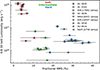 |
Fig. 1. RMS-intensity diagram: 0.8–30 keV luminosity versus fractional RMS for the systems studied in this work. The luminosity error bars are smaller than the marker size. Red, green, and blue indicate the state of the source during each observation: soft, intermediate, and hard states, respectively. The same symbol and colour code is used for all the figures. |
As shown in Fig. 1, there are a few cases where the RMS value is consistent within 1σ confidence level with more than one state. For instance, for the only observation retrieved for 4U 1916−053, the RMS is 11 ± 7%, which crosses the soft-intermediate boundary. We found evidence of two narrow absorption lines in the spectrum that were identified with absorption from Fe XXV and Fe XXVI. These features are often detected in dipping, and hence, high-inclination sources – such as 4U 1916−053 – and are interpreted as the signature of high-ionisation absorbers, revealing the presence of disc winds or atmosphere (see for reviews e.g., Díaz Trigo & Boirin 2016; Muñoz-Darias et al. 2026). These absorption lines are observed only during soft-state epochs, as proved by a thorough spectral study of the NS LMXB EXO 0748–676 (Ponti et al. 2014). Consequently, we classified the observation of 4U 1916−053 as soft state. Moreover, for 4U 1543–623 (RMS = 11 ± 5%) and the second epoch of IGR J17062–6143 (RMS = 17 ± 11%) the spectral properties disfavour a soft-state classification, while pointing towards an intermediate-state one because of the high values of the electron temperature.
Finally, for 47 Tuc X−9 and IGR J17494−3030, the RMS value is not constrained. For the former, we caught a hint of variability in the 0.1–0.5 Hz frequency range and calculated a hardness of ∼0.9, which favours a hard-state classification. The results of the spectral analysis support this claim, with a photon index of  and a luminosity level of ∼1034 erg s−1 (0.8–30 keV). For the latter, we relied on the spectral information. The best-fitting power-law with Γ = 1.92 ± 0.02 and an inferred 0.8–30 keV luminosity of ∼1035 erg s−1, together with a hardness of ∼0.55, are consistent with a hard state.
4. Discussion
We carried out a systematic study of the physical properties of the confirmed UCXBs in the hard X-rays by making use of archival NuSTAR data. We analysed 37 archival observations of 11 systems in a consistent way, adopting the same assumptions and criteria. We determined the state of the sources at a given epoch following prescriptions described in previous works and making use of RMS, hardness ratio, and spectral signatures such as narrow absorption features (see e.g., Muñoz-Darias et al. 2014; Ponti et al. 2014). Appendix B shows the NuSTAR spectra with the best-fitting models. In the following, we discuss the choice of the spectral models that can reconcile the spectral behaviour with the different states, the evolution of the spectral parameters, and the peculiar hard state of the system 4U 1626–67.
4.1. Nature of the Comptonised emission
We found that for most spectra, the best-fitting model consists of three components (i.e., bbodyrad, diskbb and nthcomp in XSPEC). Both the DISC (kTdisc = kTseed) and BB (kTBB = kTseed) approaches work, meaning that the Comptonisation seed photons may originate from the NS/boundary layer or from the accretion disc regardless of the source state. Model degeneracy is a long-standing problem that we tackled by applying performance-based criteria, listed in Section 3.2.2, following the recipe designed by Lin et al. (2007, see also Armas Padilla et al. 2017). Table 2 lists the final models that meet these requirements. Conditions 2 and 3 have already been discussed. Condition 1 can guide us towards choosing a preferable model considering the Comptonisation fraction and the RMS value (i.e., the state classification). In general, the Comptonisation fraction traces the X-ray variability, becoming higher in the hard states when accretion drops and the Comptonisation emission becomes dominant with respect to the thermal emission. We estimated the fraction of the Comptonised luminosity in the 0.8–30 keV energy range for both possible seed photon solutions. When comparing the two approaches, we noticed that the BB solution yielded lower Comptonisation fractions for most spectra in hard and intermediate states than the results from the DISC solution models. In the same way, the soft states remained weakly Comptonised if we adopted the BB solution with respect to the DISC one (with the exception of 4U 1820–303). Therefore, we used the BB approach for soft states and the DISC solution for intermediate and hard states, fulfilling Condition 1. The Comptonisation fraction estimated following this prescription as a function of the fractional RMS is shown in Fig. 2a. Within this picture, we assumed that the NS surface and/or boundary layer is the dominant supplier of seed photons for the Comptonisation process in the soft states, while the seed photons come from the disc in the other cases. Our findings are in line with the results of previous works on classical NS LMXBs. For example, Armas Padilla et al. (2017) and Sharma et al. (2018) found that for the NS LMXBs 4U 1608–52 and MXB 1658–289, respectively, in the soft state, the seed photons are provided by the NS surface/boundary layer, while in the hard state, either the disc or NS surface is equally favoured. As shown in Table 2, there are two exceptions to our modelling: MAXI J0911–655 and 4U 0614+091. The former was observed to be in the hard state at both epochs. However, only the BB approach yielded results that respect the above-mentioned conditions (see Sect. 3.2.2). We classified the first epoch of the latter as a soft state and chose the DISC approach because the BB best-fitting model gave suspicious (i.e. likely not physically meaningful) parameters for such an accretion state, namely a power-law photon index Γ of ∼4. It is important to bear in mind that our models provide a simplified picture that is only able to support one component as the dominant source of seed photons for Comptonisation, although they are most likely supplied by both the NS and accretion disc.
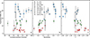 |
Fig. 2. Panel a: RMS versus fraction of Comptonised luminosity (nthcomp) estimated in the 0.8–30 keV interval. Panel b: RMS versus hardness derived as the ratio between the NuSTAR/FPMA count rates in the 10–16 keV and 6–10 keV band. Panel c: RMS versus power-law index Γ. |
In Fig. 2b, we show the hardness-RMS diagram (HRD; Belloni et al. 2005). The HRD found in this work resembles that derived by Muñoz-Darias et al. (2014, Fig. 4), who found a positive correlation between RMS and hardness until the RMS reaches values below 10–5%, where hardness increases but RMS remains constant. This trend marks a hook-shaped track in the HRD, which is a distinctive trait of NS systems. Normal atoll sources (i.e. NS LMXBs accreting below ∼30% of the Eddington luminosity) are observed to follow this peculiar hook-like path in the HRD, while the bright atolls (i.e., persistently bright systems that remain almost permanently in the bright soft states; Hasinger & van der Klis 1989) show a flat rms-hardness relation, which is similar to what we found for 4U 1820–303 (empty red stars in Fig. 2). This source is classified as an atoll, and it is persistently accreting at a relatively high luminosity, displaying mostly soft states with rare transitions to the hard states and thus behaving similar to the bright atolls. As shown in Fig. 1, 4U 1820–303 is the most luminous of our sample, with a luminosity of LX ∼ 4 × 1037 − 1038 erg s−1 (0.8–30 keV), and we always found it in soft states with an RMS between 2% and 8% and hardness in the 0.3–0.4 range. The distinctive hook shape is recovered by plotting the RMS versus the photon index Γ (Fig. 2c), and it highlights an anti-correlation between these two quantities. Generally, the soft states exhibit steeper spectra than the hard states, with 4U 1820–303 showing spectra as hard as those in the intermediate and hard states (Γ ∼ 1.8) even if the source is always observed in soft state. This hook-shaped trend might be caused by the presence of the NS surface/boundary layer contributing significantly and making the spectrum harder since it has not been seen in BH systems (e.g., Belloni et al. 2011).
Although our present dataset does not allow us to draw firm conclusions, it is worth noting a potential difference between UCXBs and longer-period NS LMXBs. The UCXBs appear not to reach the very low RMS values typically observed in classical LMXBs when they are in soft states. In Muñoz-Darias et al. (2014), 4U 1820–303 and 4U 0614+091 rarely fall below the 5% RMS level, suggesting comparatively harder soft states in UCXBs. In contrast, classical NS LMXB systems exhibit softer soft states in terms of RMS variability and possibly Comptonisation fraction. For instance, Armas Padilla et al. (2017) reported soft-state observations of the LMXB 4U 1608–52 with RMS values ∼2% and Comptonisation fractions ∼20%, while in our sample the soft states remain highly Compotonised (≥50%). These differences merit further investigation with a larger set of soft-state data.
4.2. X-ray continuum
Figure 3 shows the 0.8–30 keV luminosity as a function of the spectral parameters kTe (panel a), Γ (panel b), kTBB (panel c), and kTdisc (panel d), while Table 3 reports the weighted averaged values of the spectral parameters according to each spectral state.
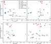 |
Fig. 3. Panel a: 0.8–30 keV luminosity versus electron temperature of the Comptonising medium kTe. Panel b: 0.8–30 keV luminosity versus power-law index Γ. Panel c: 0.8–30 keV luminosity versus blackbody temperature kTBB (=kTseed for soft-state spectra). Panel d: 0.8–30 keV luminosity versus disc temperature kTdisc (=kTseed for hard- and intermediate-state spectra). |
Weighted averages of the spectral parameters according to the spectral states.
Soft states have a kTe below ∼5 keV, excluding that of 4U 1916–053 (kTe ∼ 10 keV). For hard and intermediate states, kTe covers a larger range, extending from ∼10 keV to ≳40 keV (with the exception of 4U 1626–67, discussed below). Hard states of LMXBs have been extensively studied, revealing a dichotomy between Comptonisation properties of accreting BHs and NSs (see e.g., Burke et al. 2017; Banerjee et al. 2020). The latter have generally softer hard-state spectra than BHs because of the presence of an extra source of seed photons, that is, the NS surface. Banerjee et al. (2020) found that the kTe distribution of NS LMXBs peaks at ∼50 keV, with its 80% quantile being 16–93 keV. We note that these authors employed the model compPS (Poutanen & Svensson 1996) to describe the Comptonised emission and restricted kTe to values above 10 keV, the minimum value for which the numerical method used by the model can be expected to produce reasonable results. For the hard states of the UCXBs in our sample, the kTe values follow the expected spread, which was previously found for classical NS LMXBs, but with a lower average value of ∼20 keV, most likely due to the fact that we did not constrain the lower limit of this spectral parameter. In addition, the estimated values for Γ, kTBB (=kTseed for soft states) and kTdisc (=kTseed for hard and intermediate states) fall within the typical range of such parameters observed in other NS LMXBs at different accretion states (see Table 3; e.g., Armas Padilla et al. 2017; Sharma et al. 2018; Banerjee & Homan 2024; Ludlam et al. 2020). For completeness, we report the average values for RBB for soft, intermediate and hard states: 1.066 ± 0.005 km, 0.289 ± 0.002 km and 0.688 ± 0.003 km, respectively. We also explored possible (anti-)correlations between the spectral parameters and the orbital period, which is the property that sets UCXBs apart from classical NS LMXBs, without any success.
We can therefore conclude that the properties of the X-ray continuum in UCXBs are similar to those of their longer-period siblings. This implies that the X-ray spectral behaviour of NS LMXBs with hydrogen-rich large accretion discs is indistinguishable from that of systems with smaller discs and a different chemical composition.
4.3. 4U 1626–67: A very cold corona
We classified all the epochs of 4U 1626–67 as hard states given the high values of the RMS (see Fig. 1). Following our prescription, we chose the three-component model with the DISC approach to describe the spectra. As shown in Fig. 3a, the electron temperature values (empty blue diamonds) for this source are strikingly as low as those observed in soft states, kTe ∼ 6 keV. 4U 1626–67 is an intriguing source, even within the already exceptional UCXB family, as it is the only UCXB powered by a highly magnetised slow X-ray pulsar, with a spin period of Pspin ∼ 7.7 s. The strength of the magnetic field was derived to be ∼(3–4) × 1012 G based on a cyclotron resonance scattering feature at ∼35–37 keV.
The first epoch included in this work was already analysed by D’Aì et al. (2017), who modelled the NuSTAR dataset jointly with a Swift/XRT and Swift/BAT spectrum, thereby covering a broader energy range (0.5–150 keV). To describe the continuum, they adopted the physical model bwmodel, which is suited for the conditions in the accretion column of an accreting X-ray pulsar, and included an additional thermal (bbodyrad) and reflection (coplrefl) component. kTe, which is one of the free parameters of the model, was found to lie in the range ∼4–4.7 keV, in good agreement with our results despite the different modelling approaches. This result is to be expected on theoretical grounds, as noted by Burke et al. (2017). In the Newtonian approximation, the luminosity of the boundary layer Lbl on the NS surface is given by
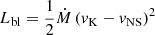
where Ṁ is the accretion rate, vK is the Keplerian velocity near the NS surface, and vNS is the linear velocity of the NS surface at the equator. The shorter the spin period (i.e. higher vNS), the smaller Lbl. In NS systems, the luminosity of seed photons Lseed is approximately equal to Lbl, and therefore systems with a shorter spin period should have a smaller Lseed. In other words, slowly rotating NSs have a higher surface luminosity and a weaker Comptonisation in the corona. They have a great supply of seed photons, implying a more efficient cooling of the corona electrons and consequently leading to colder kTe. However, we note that a further study including nine NS-LMXB systems did not find a clear correlation between the NS spin period and the electron temperature kTe (Burke et al. 2018).
5. Conclusions
We have performed a global study of UCXBs using NuSTAR observations, which covered all the classical accretion spectral states. We applied a uniform X-ray spectral analysis based on a three-component model whenever the data quality allowed for it following an approach that has become increasingly common for NS LMXBs. Our sample is the largest analysed to date with this methodology. We do not claim that our approach is either a unique solution or an adequate depiction of complexity of nature. However, it provides an overall self-consistent picture of UCXBs. Our key findings are summarised as follows:
-
The RMS-diagram of UCXBs is similar to that observed in classical NS LMXBs, including the distinctive hook-like track displayed by bright atoll sources (Muñoz-Darias et al. 2014).
-
We constrained the nature of the Comptonisation seed photons across the different accretion states, finding a behaviour consistent with that expected from NS LMXBs (e.g., Armas Padilla et al. 2017).
-
The main properties of the X-ray emission in UCXBs is not significantly different from those of NS LMXBs with longer orbital periods. This suggests that the size and chemical composition of the accretion disc do not affect the properties of the inner regions of the systems, making them uniform across different types of NS X-ray binaries.
Acknowledgments
We thank the anonymous referee for a careful reading of the paper and insightful comments. This research utilised data, software, and web tools obtained from the High Energy Astrophysics Science Archive Research Center (HEASARC), a service of the Astrophysics Science Division at NASA/GSFC. A.B. acknowledges support through the European Space Agency (ESA) research fellowship programme. T.M.D. and M.A.P. acknowledge support by the Spanish Ministry of Science via the Plan de Generacion de conocimiento PID2021-124879NB-I00 and PID2024-161863NB-I00. M.A.P. acknowledges support through the Ramn y Cajal grant RYC2022-035388-I, funded by MCIU/AEI/10.13039/501100011033 and FSE+.
References
- Anderson, S. F., Margon, B., Deutsch, E. W., Downes, R. A., & Allen, R. G. 1997, ApJ, 482, L69 [NASA ADS] [CrossRef] [Google Scholar]
- Armas Padilla, M., & López-Navas, E. 2019, MNRAS, 488, 5014 [NASA ADS] [CrossRef] [Google Scholar]
- Armas Padilla, M., Ueda, Y., Hori, T., Shidatsu, M., & Muñoz-Darias, T. 2017, MNRAS, 467, 290 [NASA ADS] [Google Scholar]
- Armas Padilla, M., Corral-Santana, J. M., Borghese, A., et al. 2023, A&A, 677, A186 [NASA ADS] [CrossRef] [EDP Sciences] [Google Scholar]
- Arnaud, K. A. 1996, Astron. Data Anal. Software Syst. V, 101, 17 [NASA ADS] [Google Scholar]
- Bachetti, M., & Huppenkothen, D. 2018, ApJ, 853, L21 [Google Scholar]
- Bahramian, A., & Degenaar, N. 2023, in Handbook of X-ray and Gamma-ray Astrophysics, eds. C. Bambi, & A. Santangelo, 120 [Google Scholar]
- Bahramian, A., Heinke, C. O., Tudor, V., et al. 2017, MNRAS, 467, 2199 [Google Scholar]
- Banerjee, S., & Homan, J. 2024, MNRAS, 529, 4311 [Google Scholar]
- Banerjee, S., Gilfanov, M., Bhattacharyya, S., & Sunyaev, R. 2020, MNRAS, 498, 5353 [NASA ADS] [CrossRef] [Google Scholar]
- Belloni, T., Homan, J., Casella, P., et al. 2005, A&A, 440, 207 [NASA ADS] [CrossRef] [EDP Sciences] [Google Scholar]
- Belloni, T. M., Motta, S. E., & Muñoz-Darias, T. 2011, Bull. Astron. Soc. India, 39, 409 [Google Scholar]
- Boirin, L., Parmar, A. N., Barret, D., Paltani, S., & Grindlay, J. E. 2004, A&A, 418, 1061 [NASA ADS] [CrossRef] [EDP Sciences] [Google Scholar]
- Bult, P. 2017, ApJ, 837, 61 [CrossRef] [Google Scholar]
- Burke, M. J., Gilfanov, M., & Sunyaev, R. 2017, MNRAS, 466, 194 [Google Scholar]
- Burke, M. J., Gilfanov, M., & Sunyaev, R. 2018, MNRAS, 474, 760 [Google Scholar]
- Chen, H.-L., Tauris, T. M., Han, Z., & Chen, X. 2021, MNRAS, 503, 3540 [NASA ADS] [CrossRef] [Google Scholar]
- Dage, K. C., Panurach, T., Oh, K., et al. 2025, ApJ, 988, 131 [Google Scholar]
- D’Aì, A., Cusumano, G., Del Santo, M., La Parola, V., & Segreto, A. 2017, MNRAS, 470, 2457 [CrossRef] [Google Scholar]
- Degenaar, N., Pinto, C., Miller, J. M., et al. 2017, MNRAS, 464, 398 [NASA ADS] [CrossRef] [Google Scholar]
- Di Marco, A., La Monaca, F., Poutanen, J., et al. 2023, ApJ, 953, L22 [NASA ADS] [CrossRef] [Google Scholar]
- Díaz Trigo, M., & Boirin, L. 2016, Astron. Nachr., 337, 368 [Google Scholar]
- Fiocchi, M., Bazzano, A., Ubertini, P., et al. 2008, A&A, 492, 557 [NASA ADS] [CrossRef] [EDP Sciences] [Google Scholar]
- Gambino, A. F., Iaria, R., Di Salvo, T., et al. 2019, A&A, 625, A92 [NASA ADS] [CrossRef] [EDP Sciences] [Google Scholar]
- Harrison, F. A., Craig, W. W., Christensen, F. E., et al. 2013, ApJ, 770, 103 [Google Scholar]
- Hasinger, G., & van der Klis, M. 1989, A&A, 225, 79 [NASA ADS] [Google Scholar]
- Huppenkothen, D., Bachetti, M., Stevens, A. L., et al. 2019, ApJ, 881, 39 [Google Scholar]
- in’t Zand, J. J. M., Jonker, P. G., & Markwardt, C. B. 2007, A&A, 465, 953 [CrossRef] [EDP Sciences] [Google Scholar]
- Kaastra, J. S., & Bleeker, J. A. M. 2016, A&A, 587, A151 [NASA ADS] [CrossRef] [EDP Sciences] [Google Scholar]
- Koliopanos, F., Péault, M., Vasilopoulos, G., & Webb, N. 2021, MNRAS, 501, 548 [Google Scholar]
- Kubota, A., Tanaka, Y., Makishima, K., et al. 1998, PASJ, 50, 667 [NASA ADS] [CrossRef] [Google Scholar]
- Lasota, J.-P. 2001, New Astron. Rev., 45, 449 [Google Scholar]
- Li, Z. S., Kuiper, L., Falanga, M., et al. 2021, A&A, 649, A76 [NASA ADS] [CrossRef] [EDP Sciences] [Google Scholar]
- Lin, D., Remillard, R. A., & Homan, J. 2007, ApJ, 667, 1073 [CrossRef] [Google Scholar]
- Ludlam, R. M., Miller, J. M., Barret, D., et al. 2019, ApJ, 873, 99 [Google Scholar]
- Ludlam, R. M., Cackett, E. M., García, J. A., et al. 2020, ApJ, 895, 45 [NASA ADS] [CrossRef] [Google Scholar]
- Ludlam, R. M., Jaodand, A. D., García, J. A., et al. 2021, ApJ, 911, 123 [Google Scholar]
- Marino, A., Russell, T. D., Del Santo, M., et al. 2023, MNRAS, 525, 2366 [NASA ADS] [CrossRef] [Google Scholar]
- Mitsuda, K., Inoue, H., Koyama, K., et al. 1984, PASJ, 36, 741 [NASA ADS] [Google Scholar]
- Mitsuda, K., Inoue, H., Nakamura, N., & Tanaka, Y. 1989, PASJ, 41, 97 [NASA ADS] [Google Scholar]
- Mondal, A. S., Dewangan, G. C., Pahari, M., et al. 2016, MNRAS, 461, 1917 [Google Scholar]
- Moutard, D., Ludlam, R., García, J. A., et al. 2023, ApJ, 957, 27 [NASA ADS] [CrossRef] [Google Scholar]
- Muñoz-Darias, T., Motta, S., & Belloni, T. M. 2011, MNRAS, 410, 679 [Google Scholar]
- Muñoz-Darias, T., Fender, R. P., Motta, S. E., & Belloni, T. M. 2014, MNRAS, 443, 3270 [CrossRef] [Google Scholar]
- Muñoz-Darias, T., Díaz Trigo, M., Done, C., Ponti, G., & Tomaru, R. 2026, ArXiv e-prints [arXiv:2601.05319] [Google Scholar]
- Nelemans, G., Wood, M., Groot, P., et al. 2009, astro2010: The Astronomy and Astrophysics Decadal Survey, 2010, 221 [Google Scholar]
- Orlandini, M., Dal Fiume, D., Frontera, F., et al. 1998, ApJ, 500, L163 [NASA ADS] [CrossRef] [Google Scholar]
- Ponti, G., Muñoz-Darias, T., & Fender, R. P. 2014, MNRAS, 444, 1829 [NASA ADS] [CrossRef] [Google Scholar]
- Popham, R., & Sunyaev, R. 2001, ApJ, 547, 355 [NASA ADS] [CrossRef] [Google Scholar]
- Poutanen, J., & Svensson, R. 1996, ApJ, 470, 249 [CrossRef] [Google Scholar]
- Rappaport, S., Markert, T., Li, F. K., et al. 1977, ApJ, 217, L29 [NASA ADS] [CrossRef] [Google Scholar]
- Rappaport, S., Joss, P. C., & Webbink, R. F. 1982, ApJ, 254, 616 [NASA ADS] [CrossRef] [Google Scholar]
- Sanna, A., Papitto, A., Burderi, L., et al. 2017, A&A, 598, A34 [NASA ADS] [CrossRef] [EDP Sciences] [Google Scholar]
- Sanna, A., Bahramian, A., Bozzo, E., et al. 2018a, A&A, 610, L2 [NASA ADS] [CrossRef] [EDP Sciences] [Google Scholar]
- Sanna, A., Pintore, F., Riggio, A., et al. 2018b, MNRAS, 481, 1658 [NASA ADS] [CrossRef] [Google Scholar]
- Sharma, R. 2025, J. High Energy Astrophys., 47, 100376 [Google Scholar]
- Sharma, R., Jaleel, A., Jain, C., et al. 2018, MNRAS, 481, 5560 [Google Scholar]
- Sharma, R., Jain, C., & Paul, B. 2023, MNRAS, 526, L35 [NASA ADS] [CrossRef] [Google Scholar]
- Sharma, R., Jain, C., Paul, B., & Beri, A. 2025, MNRAS, 538, 1046 [Google Scholar]
- Shimura, T., & Takahara, F. 1995, ApJ, 445, 780 [Google Scholar]
- Smale, A. P., Mason, K. O., White, N. E., & Gottwald, M. 1988, MNRAS, 232, 647 [Google Scholar]
- Stoop, M., van den Eijnden, J., Degenaar, N., et al. 2021, MNRAS, 507, 330 [NASA ADS] [CrossRef] [Google Scholar]
- Tobrej, M., Tamang, R., Rai, B., Ghising, M., & Paul, B. C. 2024, MNRAS, 528, 3550 [Google Scholar]
- van den Eijnden, J., Degenaar, N., Pinto, C., et al. 2018, MNRAS, 475, 2027 [Google Scholar]
- van Paradijs, J., & McClintock, J. E. 1994, A&A, 290, 133 [NASA ADS] [Google Scholar]
- Verner, D. A., Ferland, G. J., Korista, K. T., & Yakovlev, D. G. 1996, ApJ, 465, 487 [Google Scholar]
- Walter, F. M., Mason, K. O., Clarke, J. T., et al. 1982, ApJ, 253, L67 [NASA ADS] [CrossRef] [Google Scholar]
- Wilms, J., Allen, A., & McCray, R. 2000, ApJ, 542, 914 [Google Scholar]
- Zdziarski, A. A., Johnson, W. N., & Magdziarz, P. 1996, MNRAS, 283, 193 [NASA ADS] [CrossRef] [Google Scholar]
- Życki, P. T., Done, C., & Smith, D. A. 1999, MNRAS, 309, 561 [Google Scholar]
We considered observations acquired up to July 2023.
NuSTAR Calibration Update: https://nustarsoc.caltech.edu/NuSTAR_Public/NuSTAROperationSite/CALDB20211020.php
Condition 3 is met for all epochs of 4U 1820−303, 4U 1543−624, MAXI J0911−655, and 4U 1916−053; only for the first epoch of 4U J1626−67 and Swift J1756.9−2508; only for the third epoch of IGR J17062−6143; for all epochs apart from the fourth one of 4U 0614+091. Note that (i) we did not consider the distance error (not always known) when deriving the uncertainty of Rdisc and (ii)RNS= 10 km was assumed.
Appendix A: Log of observations
This section provides the log of the NuSTAR observations that were analysed in this work. Each table lists
– the observation start time;
– the exposure time for FPMA after filtering for type-I X-ray bursts and background flaring events;
– the source background-subtracted count rate in the 3–15 keV energy band for FPMA. We chose this energy band because all the sources are detected between 3 and 15 keV. The only exception is 47 Tuc X−9: this object is the dominant source of X-rays above 6 keV in the cluster, therefore we considered the 6–15 keV interval to minimise the contamination (Bahramian et al. 2017);
– 0.8-30 keV luminosity from the unabsorbed flux obtained from the best-fitting model and distance reported in Table 1;
– references to the papers where the observation was analysed for the first time for either spectral or timing studies.
X-ray observation log.
Appendix B: NuSTAR spectra and fitted models
This section reports the NuSTAR spectra with the best-fitting models. In each case, we plot the E × f(E) unfolded spectra and the model with the single components. Post-fit residuals in units of standard deviations are also plotted at the bottom of each panel. Same symbol/colour code is used for all the figures: black dots for FPMA data, grey circle for FPMB data, dashed blue line for the blackbody component, dotted green line for the disk component, dash-dotted orange line for the thermally Comptonised continuum component and yellow for the iron line. In a few spectra, one or more components do not appear in the plot, because their contributions fall outside the plotted flux range.
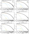 |
Fig. B.1. Spectra of 4U 1820–303. |
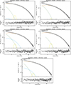 |
Fig. B.2. continued. |
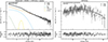 |
Fig. B.3. Left: Spectrum of 4U 1543–624. Right: Spectrum of 47 Tuc X−9. |
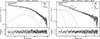 |
Fig. B.4. Left: Spectrum of IGR J16597−3704. Right: Spectrum of 4U 1916−053. |
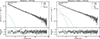 |
Fig. B.5. Spectra of MAXI J0911−655. |
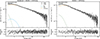 |
Fig. B.6. Spectra of Swift J1756.9−2508. |
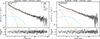 |
Fig. B.7. Spectra of IGR J17062−6143 for the first (left) and second (right) epoch. |
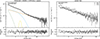 |
Fig. B.8. Left: Spectrum of IGR J17062−6143 for the third epoch. Right: Spectrum of IGR J17494−3030. |
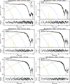 |
Fig. B.9. Spectra of 4U 1626−67. |
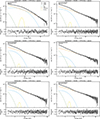 |
Fig. B.10. Spectra of 4U 0614+091. |
All Tables
Main properties of the UCXBs included in this work. The sources are sorted by increasing orbital period.
All Figures
|
Fig. 1. RMS-intensity diagram: 0.8–30 keV luminosity versus fractional RMS for the systems studied in this work. The luminosity error bars are smaller than the marker size. Red, green, and blue indicate the state of the source during each observation: soft, intermediate, and hard states, respectively. The same symbol and colour code is used for all the figures. |
| In the text | |
|
Fig. 2. Panel a: RMS versus fraction of Comptonised luminosity (nthcomp) estimated in the 0.8–30 keV interval. Panel b: RMS versus hardness derived as the ratio between the NuSTAR/FPMA count rates in the 10–16 keV and 6–10 keV band. Panel c: RMS versus power-law index Γ. |
| In the text | |
|
Fig. 3. Panel a: 0.8–30 keV luminosity versus electron temperature of the Comptonising medium kTe. Panel b: 0.8–30 keV luminosity versus power-law index Γ. Panel c: 0.8–30 keV luminosity versus blackbody temperature kTBB (=kTseed for soft-state spectra). Panel d: 0.8–30 keV luminosity versus disc temperature kTdisc (=kTseed for hard- and intermediate-state spectra). |
| In the text | |
|
Fig. B.1. Spectra of 4U 1820–303. |
| In the text | |
|
Fig. B.2. continued. |
| In the text | |
|
Fig. B.3. Left: Spectrum of 4U 1543–624. Right: Spectrum of 47 Tuc X−9. |
| In the text | |
|
Fig. B.4. Left: Spectrum of IGR J16597−3704. Right: Spectrum of 4U 1916−053. |
| In the text | |
|
Fig. B.5. Spectra of MAXI J0911−655. |
| In the text | |
|
Fig. B.6. Spectra of Swift J1756.9−2508. |
| In the text | |
|
Fig. B.7. Spectra of IGR J17062−6143 for the first (left) and second (right) epoch. |
| In the text | |
|
Fig. B.8. Left: Spectrum of IGR J17062−6143 for the third epoch. Right: Spectrum of IGR J17494−3030. |
| In the text | |
|
Fig. B.9. Spectra of 4U 1626−67. |
| In the text | |
|
Fig. B.10. Spectra of 4U 0614+091. |
| In the text | |
Current usage metrics show cumulative count of Article Views (full-text article views including HTML views, PDF and ePub downloads, according to the available data) and Abstracts Views on Vision4Press platform.
Data correspond to usage on the plateform after 2015. The current usage metrics is available 48-96 hours after online publication and is updated daily on week days.
Initial download of the metrics may take a while.