| Issue |
A&A
Volume 710, June 2026
|
|
|---|---|---|
| Article Number | A93 | |
| Number of page(s) | 7 | |
| Section | Numerical methods and codes | |
| DOI | https://doi.org/10.1051/0004-6361/202659861 | |
| Published online | 03 June 2026 | |
A user-friendly package and workflow for generating effective homogeneous rheologies for the study of the long-term orbital evolution of multilayered planetary bodies
King Abdullah University of Science and Technology (KAUST),
Thuwal,
Saudi Arabia
★ Corresponding author: This email address is being protected from spambots. You need JavaScript enabled to view it.
Received:
14
March
2026
Accepted:
30
April
2026
Abstract
Context. Tidal dissipation plays an important role in the long-term orbital evolution of planets and moons. For stratified viscoelastic bodies, evaluating the frequency-dependent tidal response during long-term dynamical integrations is computationally expensive, since it requires repeatedly solving the internal deformation problem. Therefore, orbital evolution codes benefit from effective homogeneous rheologies that approximate the dissipation of stratified interiors at low computational cost.
Aims. We present a user-friendly, open-source Wolfram Language package that constructs an effective homogeneous generalized Voigt rheology for a spherically symmetric, incompressible layered body with Maxwell solid layers. The package converts the tidal response of a layered interior model into the parameters required by time-domain simulations of tidal evolution.
Methods. The package combines three components: (i) a forward computation of the degree-2 tidal Love number based on the propagator-matrix formulation for incompressible stratified viscoelastic bodies; (ii) numerical identification of the secular relaxation poles and residues of the layered model; and (iii) inversion of the resulting response into the compliance of an equivalent homogeneous generalized Voigt body. The implementation is based on the equivalence established for multilayer Maxwell bodies and includes an optional dominant-mode selection procedure for obtaining reduced rheological models over a prescribed frequency range.
Results. The package returns the parameters of the equivalent homogeneous model, including elastic, gravitational, viscous, and Voigt-element contributions, in a format that can be used by external tidal-evolution codes. As a case study, we apply the package to a five-layer lunar interior model and obtain its equivalent generalized Voigt representation, together with a reduced model that preserves the tidal response over the frequency interval relevant for orbital evolution while using fewer relaxation elements.
Conclusions. The package provides a reproducible implementation of the reduction from stratified viscoelastic interiors to effective homogeneous rheologies. It allows tidal dissipation from layered models to be included in long-term orbital and spin-evolution calculations without solving the full layered boundary-value problem at each step.
Key words: methods: numerical / planets and satellites: dynamical evolution and stability / planets and satellites: interiors
© The Authors 2026
 Open Access article, published by EDP Sciences, under the terms of the Creative Commons Attribution License (https://creativecommons.org/licenses/by/4.0), which permits unrestricted use, distribution, and reproduction in any medium, provided the original work is properly cited.
This article is published in open access under the Subscribe to Open model. This email address is being protected from spambots. You need JavaScript enabled to view it. to support open access publication.
1 Introduction
Tidal deformation and energy dissipation play an important role in the long-term orbital evolution of planets and moons. The magnitude and frequency of tidal dissipation depend on the internal structure of the deformable body, in particular on the distribution of density, elasticity, and viscosity.
Tidal deformation is modeled with the frequency-dependent degree-2 tidal Love number k2(s), which can be obtained by solving the governing equations for a radially stratified viscoelastic body. Here, the stratified forward model follows the propagatormatrix formulation for incompressible, spherically symmetric stratified bodies in Sabadini et al. (2016, Chapter 2). Solid layers are modeled with Maxwell rheology and liquid layers through the appropriate small-shear limit. This approach is a consistent way to evaluate the tidal response of the body, but it can become too costly to solve repeatedly within long-term orbital or spin-evolution integrations.
Long-term dynamical evolution codes often rely on simplified homogeneous rheologies or empirical prescriptions, such as constant time lag, constant phase lag, or single-element Maxwell models. These approximations are computationally convenient but generally fail to reproduce the multiple relaxation timescales and dissipation peaks that arise in layered bodies Gevorgyan (2021); Bolmont et al. (2020). In Gevorgyan et al. (2023), the authors showed that, under the assumptions of a simple multilayer rheology, the tidal response of a stratified body can be modeled by a homogeneous body with a sufficiently complex generalized rheology, such as a generalized Voigt model. This motivated us to develop a relatively simple workflow that allows one to replace the stratified problem by an effective homogeneous model that preserves the frequency-dependent tidal response.
In this work, we present an open-source Wolfram Language package1 that takes a user-specified multilayered model and constructs the corresponding effective homogeneous generalized Voigt rheology. The input file contains the layer radii, densities, shear moduli, viscosities, and forcing frequency, and the main routine performs the full reduction pipeline: computation of k2(s) for the layered model, identification of secular poles and residues, inversion to the equivalent compliance function, and extraction of the generalized Voigt parameters. An optional reduction step identifies dominant relaxation modes over a user-defined frequency interval, yielding a compact model when an exact full representation is unnecessary.
Our implementation was partly motivated by the need to connect detailed geophysical interior models with modern time-domain orbital integrators such as the RheoVolution (de Oliveira et al. 2025a,b), which can evolve deformable bodies with complex homogeneous rheologies, but require as input the parameters of an effective rheological model rather than a full multilayer interior description. The package converts the tidal response of a stratified viscoelastic body into the parameters of a homogeneous generalized Voigt model that can be used in such simulations.
The paper is organized as follows. In Section 2, we summarize the theoretical framework for effective homogeneous rheology and its relation to the layered tidal response. In Section 3, we describe the structure of the software package, its inputs and outputs, and the computational workflow. In Section 4, we illustrate the method with an application to a five-layer model of the Moon and show how the package recovers the equivalent generalized Voigt rheology and, if desired, an optional reduced model that captures the tidal response over the frequency interval of interest. In Section 5 we conclude the paper with observations on the purpose and scope of the work and a few perspectives for improvement.
2 Theoretical background
This section summarizes the theoretical elements relevant to the software pipeline. The forward computation of the layered tidal response follows the propagator-matrix formulation for incompressible, stratified viscoelastic bodies presented in Sabadini et al. (2016), while the reduction to an equivalent homogeneous rheology is based on Gevorgyan et al. (2023).
2.1 Layered viscoelastic model
If we consider a spherically symmetric body of N incompressible, homogeneous layers, each with outer radius rk, density ρk, rigidity μk, and viscosity ηk, solid layers are assumed to have Maxwell rheology, and their complex shear modulus in the Laplace domain is
![Mathematical equation: $\[\hat{\mu}_k(s)=\frac{\mu_k \eta_k s}{\mu_k+\eta_k s}.\]$](/articles/aa/full_html/2026/06/aa59861-26/aa59861-26-eq1.png) (1)
(1)
The tidal response is described by the degree-2 Love number k2(s), obtained from the propagator-matrix solution of the governing equations for a stratified body. All layers are treated within a unified propagator formulation, and liquid layers are treated in the small-shear limit; see Section 3.3.
For a finite multilayer Maxwell body, k2(s) is a rational function of the Laplace variable and admits the mode decomposition (Gevorgyan et al. 2023, Eq. (26))
![Mathematical equation: $\[k_2(s)=k_E+\sum_{i=1}^{n+1} \frac{r_i}{s-s_i},\]$](/articles/aa/full_html/2026/06/aa59861-26/aa59861-26-eq2.png) (2)
(2)
where kE is the elastic Love number, si < 0 are the secular poles, ri are the corresponding residues and ![Mathematical equation: $\[\tau_{i}=-s_{i}^{-1}\]$](/articles/aa/full_html/2026/06/aa59861-26/aa59861-26-eq3.png) are the relaxation times. Here n denotes the number of Kelvin–Voigt elements of the equivalent homogeneous model, so the layered body has n + 1 normal modes, in agreement with Gevorgyan et al. (2023, Eq. (22)). Thus, the layered tidal response is fully characterized by the set of parameters {kE, si, ri}.
are the relaxation times. Here n denotes the number of Kelvin–Voigt elements of the equivalent homogeneous model, so the layered body has n + 1 normal modes, in agreement with Gevorgyan et al. (2023, Eq. (22)). Thus, the layered tidal response is fully characterized by the set of parameters {kE, si, ri}.
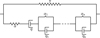 |
Fig. 1 Schematic representation of the generalized Voigt model. |
2.2 The homogeneous model
The equivalent homogeneous representation of stratified bodies is given by a generalized Voigt rheology in Figure 1. The Love number of the body is (Gevorgyan et al. 2023, Eq. (2))
![Mathematical equation: $\[k_2(s)=\frac{3 \mathrm{I}_{\circ} G}{R^5} C(s),\]$](/articles/aa/full_html/2026/06/aa59861-26/aa59861-26-eq4.png) (3)
(3)
where I° is the mean moment of inertia, C(s) is the complex compliance, and R is the mean radius of the body. The gravitational rigidity γ is defined from the fluid Love number kf as (Gevorgyan et al. 2023, Eq. (4))
![Mathematical equation: $\[\gamma=\frac{3 \mathrm{I}_{\circ} G}{R^5} \frac{1}{k_f}.\]$](/articles/aa/full_html/2026/06/aa59861-26/aa59861-26-eq5.png) (4)
(4)
For generalized Voigt rheology, complex compliance is decomposed as (Gevorgyan et al. 2023, Eq. (14))
![Mathematical equation: $\[C(s)=\frac{1}{\alpha+\gamma}+C_v(s),\]$](/articles/aa/full_html/2026/06/aa59861-26/aa59861-26-eq6.png) (5)
(5)
where α is the elastic rigidity and Cv(s) contains the viscous contribution of the dashpot and a finite number of Kelvin–Voigt elements in Figure 1. The equivalent homogeneous model is specified by the parameters {γ, α, η, αi, ηi}. In these expressions γ, α, and αi have dimensions of s−2, as does the mapping constant Θ = 3I°G/R5, while η and ηi have dimensions of s−1. To convert to SI units of Pa and Pa s, we divide by the rescaling factor ![Mathematical equation: $\[\frac{152 \pi}{15} \frac{R}{m_{1}}\]$](/articles/aa/full_html/2026/06/aa59861-26/aa59861-26-eq7.png) (Gevorgyan et al. 2020, Section 7.1.1), where m1 is the mass of the body. The outputs reported by the package (for example, in Table 6) are given in these units.
(Gevorgyan et al. 2020, Section 7.1.1), where m1 is the mass of the body. The outputs reported by the package (for example, in Table 6) are given in these units.
2.3 Extraction of the homogeneous model parameters
The parameters of the equivalent homogeneous generalized Voigt rheology are obtained from the layered pole–residue data ![Mathematical equation: $\[\left\{k_{E}, s_{i}, r_{i}\right\}_{i=1}^{n+1}\]$](/articles/aa/full_html/2026/06/aa59861-26/aa59861-26-eq8.png) by a purely algebraic procedure. Writing the layered compliance
by a purely algebraic procedure. Writing the layered compliance
![Mathematical equation: $\[C_L(s)=\frac{R^5}{3 I_{\circ} G} k_2(s)=k_E^C+\sum_{i=1}^{n+1} \frac{r_i^C}{s-s_i},\]$](/articles/aa/full_html/2026/06/aa59861-26/aa59861-26-eq9.png) (6)
(6)
where ![Mathematical equation: $\[k_{E}^{C}\]$](/articles/aa/full_html/2026/06/aa59861-26/aa59861-26-eq10.png) and
and ![Mathematical equation: $\[r_{i}^{C}\]$](/articles/aa/full_html/2026/06/aa59861-26/aa59861-26-eq11.png) are kE and ri rescaled by R5/(3I°G), the elastic and gravitational parameters follow from the asymptotic limits of compliance,
are kE and ri rescaled by R5/(3I°G), the elastic and gravitational parameters follow from the asymptotic limits of compliance,
![Mathematical equation: $\[\gamma=\left(k_E^C-\sum_{i=1}^{n+1} \frac{r_i^C}{s_i}\right)^{-1}, \qquad \alpha=\frac{1}{k_E^C}-\gamma.\]$](/articles/aa/full_html/2026/06/aa59861-26/aa59861-26-eq12.png) (7)
(7)
The remaining parameters are η and the n Kelvin–Voigt pairs ![Mathematical equation: $\[\left\{\left(\alpha_{i}, \eta_{i}\right)\right\}_{i=1}^{n}\]$](/articles/aa/full_html/2026/06/aa59861-26/aa59861-26-eq13.png) , totaling 2n + 1 unknowns. Attempting to extract these parameters from the n + 1 pole conditions of the generalized Voigt model would be both underdetermined and nonlinear. Instead, we construct the complex compliance of the viscoelastic element
, totaling 2n + 1 unknowns. Attempting to extract these parameters from the n + 1 pole conditions of the generalized Voigt model would be both underdetermined and nonlinear. Instead, we construct the complex compliance of the viscoelastic element ![Mathematical equation: $\[\hat{J}(s)\]$](/articles/aa/full_html/2026/06/aa59861-26/aa59861-26-eq14.png) (Gevorgyan et al. 2023, Eq. (13)),
(Gevorgyan et al. 2023, Eq. (13)),
![Mathematical equation: $\[\hat{J}(s)=\frac{1}{\alpha}+\frac{1}{\eta s}+\sum_{i=1}^n \frac{1}{\alpha_i+s \eta_i},\]$](/articles/aa/full_html/2026/06/aa59861-26/aa59861-26-eq15.png) (8)
(8)
directly from the layered data through the relation ![Mathematical equation: $\[C^{-1}(s)=\gamma+ \hat{J}^{-1}(s)\]$](/articles/aa/full_html/2026/06/aa59861-26/aa59861-26-eq16.png) , which yields
, which yields
![Mathematical equation: $\[\hat{J}(s)=\frac{C_L(s)}{1-\gamma C_L(s)}.\]$](/articles/aa/full_html/2026/06/aa59861-26/aa59861-26-eq17.png) (9)
(9)
All Kelvin–Voigt parameters are then read off from the partial-fraction decomposition of ![Mathematical equation: $\[\hat{J}(s)\]$](/articles/aa/full_html/2026/06/aa59861-26/aa59861-26-eq18.png) .
.
Writing the layered compliance (6) as a single fraction CL(s) = N(s)/D(s), where ![Mathematical equation: $\[D(s)={\prod}_{i=1}^{n+1}\left(s-s_{i}\right)\]$](/articles/aa/full_html/2026/06/aa59861-26/aa59861-26-eq19.png) and N(s) is a polynomial of degree n + 1, Equation (9) gives
and N(s) is a polynomial of degree n + 1, Equation (9) gives
![Mathematical equation: $\[\hat{J}(s)=\frac{N(s)}{D(s)-\gamma N(s)}=\frac{N(s)}{s Q(s)},\]$](/articles/aa/full_html/2026/06/aa59861-26/aa59861-26-eq20.png) (10)
(10)
where the denominator vanishes at s = 0 as a direct consequence of the definition of γ in Eq. (7), and Q(s) is a polynomial of degree n. The poles of ![Mathematical equation: $\[\hat{J}(s)\]$](/articles/aa/full_html/2026/06/aa59861-26/aa59861-26-eq21.png) are therefore s = 0 and the n roots of Q(s), which are real, negative, and simple (from the interlacing property in Eq. (22) of Gevorgyan et al. 2023).
are therefore s = 0 and the n roots of Q(s), which are real, negative, and simple (from the interlacing property in Eq. (22) of Gevorgyan et al. 2023).
The residue of ![Mathematical equation: $\[\hat{J}(s)\]$](/articles/aa/full_html/2026/06/aa59861-26/aa59861-26-eq22.png) at s = 0 comes entirely from the dashpot term in Eq. (8), the only singular contribution at the origin. Matching the residue computed from Eq. (10) gives
at s = 0 comes entirely from the dashpot term in Eq. (8), the only singular contribution at the origin. Matching the residue computed from Eq. (10) gives
![Mathematical equation: $\[\eta=\frac{Q(0)}{N(0)}.\]$](/articles/aa/full_html/2026/06/aa59861-26/aa59861-26-eq23.png) (11)
(11)
At each remaining pole qi, only the i-th Kelvin–Voigt term is singular, and writing ![Mathematical equation: $\[1 /\left(\alpha_{i}+s \eta_{i}\right)=\eta_{i}^{-1} /\left(s-q_{i}\right)\]$](/articles/aa/full_html/2026/06/aa59861-26/aa59861-26-eq24.png) with qi = −αi/ηi, residue matching yields
with qi = −αi/ηi, residue matching yields
![Mathematical equation: $\[\eta_i=\frac{q_i ~Q^{\prime}(q_i)}{N(q_i)}, \quad \alpha_i=-q_i \eta_i=\frac{-q_i^2 ~Q^{\prime}(q_i)}{N(q_i)}.\]$](/articles/aa/full_html/2026/06/aa59861-26/aa59861-26-eq25.png) (12)
(12)
No nonlinear system is solved. The only numerical step is the polynomial root-finding of Q(s), a standard operation for a polynomial whose roots are real, negative, and simple. For a layered body with n + 1 normal modes, the 2n + 3 data points ![Mathematical equation: $\[\left\{k_{E}^{C}, r_{i}^{C}, s_{i}\right\}\]$](/articles/aa/full_html/2026/06/aa59861-26/aa59861-26-eq26.png) uniquely determine the 2n + 3 parameters {γ, α, η, αi, ηi} of the equivalent homogeneous model.
uniquely determine the 2n + 3 parameters {γ, α, η, αi, ηi} of the equivalent homogeneous model.
3 Software implementation and workflow
The package is written in Wolfram Language as a modular pipeline for constructing the homogeneous generalized Voigt rheology of a layered viscoelastic body. The model is not hardcoded to any specific planetary interior: all physical and numerical inputs are supplied by the user through a configuration file, and the same workflow applies to any incompressible, spherically symmetric multilayer model satisfying the assumptions discussed in Section 2.
3.1 Package structure
The code is organized into a small set of modules with distinct roles. The file ModelInput.wl contains the user-specified physical model and numerical settings. The core routines are called by computeHomogeneous, implemented in HomogeneousRheology.wl, which evaluates the layered tidal response, extracts the secular poles and residues, and returns the parameters of the equivalent generalized Voigt model. A driver script, RunHomogeneous.wl, loads the modules, executes the full pipeline, prints summary tables, and generates comparison plots. A separate script, VisualizeLayers.wl, produces a cross-sectional visualization of the layered body directly from the same input file.
3.2 Input configuration
The file ModelInput.wl contains both the physical description of the layered body and a small set of numerical controls for the inversion pipeline. The same workflow can be applied to any spherically symmetric multilayer configuration once the corresponding layer properties and forcing frequency are provided.
The physical model is specified through the arrays of outer radii, densities, rigidities, and viscosities of the layers, together with the tidal forcing frequency. An optional list of layer names may be supplied for visualization purposes. All physical quantities are given in SI units, and all arrays must have the same length, which determines the number of layers in the model. Liquid layers are identified by the condition 0 < μ < 1 Pa; for such layers, the method uses an effective elasticity value to regularize the small-shear limit (Sabadini et al. 2016).
The same input file contains numerical settings that control the precision of the calculations, the search interval used to detect the secular poles, and the frequency range and threshold adopted in the dominant-mode selection step. These parameters are not part of the planetary model but determine how the software resolves the relaxation spectrum and how aggressively the final generalized Voigt model is reduced. Their default values are listed in Table 1.
The single tidal forcing frequency ω and the frequency interval [ωmin, ωmax] play distinct roles. The rheological parameters of the equivalent homogeneous model are frequencyindependent, determined entirely by the secular poles and residues of the layered k2(s). The single ω is used only to evaluate and report k2(iω) at the frequency of interest for the body under consideration. For the Moon, this corresponds to the orbital frequency ω = 2.662 × 10⁻⁶ rad s−1, associated with the 27.32-day orbital period, which we use throughout the case study in Section 4. The interval [ωmin, ωmax] enters only in the optional dominant-mode reduction step, where it defines the band over which each Kelvin–Voigt element is assessed for retention in the reduced model.
3.3 Main routine and computational workflow
The main routine
computeHomogeneous[rk,rhok,muk,etak,omega,opts]
performs the parameter extraction through the sequence of operations illustrated in Fig. 2. It follows the same three-step structure as in Sections 1 and 2: forward computation of the layered Love number, mode decomposition, and rheological inversion. The code first evaluates the elastic Love number kE and the complex tidal response k2(iω) for the layered body. It then searches for the zeros of the secular determinant on the negative real axis, refines them numerically, and computes the corresponding residues. From these quantities, it evaluates the fluid Love number kf and the mapping constant Θ = 3I°G/R5, and applies the algebraic procedure of Section 2.3 to extract the parameters {γ, α, η, αi, ηi} of the equivalent generalized Voigt model.
The forward layered problem is evaluated through a unified 6 × 6 propagator matrix approach for all layers. Liquid layers are treated by small-shear regularization, such that solid and liquid regions are handled within the same numerical framework. The current package does not switch to a separate Clairaut propagator for liquids, but instead uses a single propagation formalism for arbitrary combinations of solid and liquid layers. A true liquid has μ = 0, but the Y-matrix (Sabadini et al. 2016, Eq. (2.42)) contains terms of the form μ/r in rows 3, 4, and 6. Setting μ = 0 exactly would therefore cause these rows to degenerate, causing the linear solver to fail when computing the propagator
![Mathematical equation: $\[P(r_2, r_1)=Y(r_2) Y^{-1}(r_1).\]$](/articles/aa/full_html/2026/06/aa59861-26/aa59861-26-eq27.png) (13)
(13)
Instead, we assign a very small effective rigidity ![Mathematical equation: $\[\hat{\mu} \approx 10^{-20} \mathrm{~Pa}\]$](/articles/aa/full_html/2026/06/aa59861-26/aa59861-26-eq28.png) to the liquid layers. This keeps the matrix full-rank and invertible, while making the shear-stress rows effectively zero to machine precision. This value is negligible compared to the physical shear moduli, which are typically of the order of 109−1011 Pa, but remains large enough to preserve numerical stability at all reasonable (actually, even at quite stringent) working precisions. This is a standard regularization in viscoelastic normal-mode calculations that avoids introducing a separate 2 × 2 or 4 × 4 propagator for liquid layers while yielding results indistinguishable from the inviscid limit to within working precision.
to the liquid layers. This keeps the matrix full-rank and invertible, while making the shear-stress rows effectively zero to machine precision. This value is negligible compared to the physical shear moduli, which are typically of the order of 109−1011 Pa, but remains large enough to preserve numerical stability at all reasonable (actually, even at quite stringent) working precisions. This is a standard regularization in viscoelastic normal-mode calculations that avoids introducing a separate 2 × 2 or 4 × 4 propagator for liquid layers while yielding results indistinguishable from the inviscid limit to within working precision.
After the full generalized Voigt model is obtained, the package performs an optional dominant-mode reduction, following the criterion introduced in Gevorgyan et al. (2023, Appendix A). For each Voigt element, it evaluates the maximum fractional contribution to – Im[C(iω)] over a user-defined frequency interval [ωmin, ωmax]. Elements whose contribution exceeds the prescribed threshold are kept in the reduced model. This produces a compact, effective rheology targeted to the frequency interval most relevant for the intended dynamical application.
Main user inputs and numerical controls of the Wolfram package.
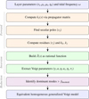 |
Fig. 2 Workflow of the computeHomogeneous pipeline. |
3.4 Output
The main routine computeHomogeneous returns the layered response and its homogeneous representation as a Wolfram Association, and also exports the corresponding results to a JSON file. The package also returns the intermediate modes used in the inversion. In this way, the user has access both to the physical outputs of interest – the effective generalized Voigt parameters – and to the pole–residue decomposition that connects the layered model to the homogeneous model. The quantities returned are summarized in Table 2.
The output falls into three groups: the Love numbers of the layered body, the constants used in the layered-to-homogeneous mapping, and the relaxation modes and rheological parameters of the equivalent generalized Voigt model. This organization separates diagnostic quantities from the final effective model. The Love-number and mode outputs are used to check the inversion, and the generalized Voigt parameters are used in downstream applications. The package also generates summary tables, dominant-mode diagnostics, and comparison plots. The user can inspect the mode decomposition, compare the full and reduced models, or export the reduced generalized Voigt parameters to an external integrator such as RheoVolution (de Oliveira et al. 2025a,b).
Quantities returned by computeHomogeneous.
4 Case study: A five-layer model of the Moon
To test the package, we used the five-layer lunar model of Gevorgyan et al. (2023) to illustrate the equivalence between a multilayer Maxwell body and an effective homogeneous rheology. The model parameters are summarized in Table 3, and its cross-section is illustrated in Fig. 3; the figure was automatically produced by the VisualizeLayers.wl module. The Moon is the default example configuration in the package. The package was also tested for Io, Europa, and Enceladus using models and data from Hussmann & Spohn (2004), Wahr et al. (2006), Bierson & Nimmo (2016), and Thomas et al. (2016), although we are only going to report the results for the Moon. The ModelInput files for these additional test cases can be found in the software package repository.
Physical parameters for the five-layer viscoelastic model of the lunar interior.
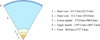 |
Fig. 3 Cross-section depiction of the five-layer lunar interior model automatically generated by the VisualizeLayers.wl routine. The numbered list indicates the thickness of each corresponding layer, along with the position (radius) of its outer boundary in parentheses. |
Secular relaxation modes extracted for the five-layer lunar model.
4.1 The homogeneous model
The software extracts the secular relaxation poles and residues listed in Table 4. These modes provide the normal-mode decomposition of the lunar tidal response and are used to construct the equivalent homogeneous rheology. The corresponding inversion yields the full equivalent generalized Voigt model, whose parameters are listed in Tables 5 and 6.
In Figure 4, we compare the dissipative part – Im[k2(iω)] and the elastic part, Re[k2(iω)], of the layered moon model to the full homogeneous model. The agreement shows that the full equivalent generalized Voigt model reproduces both the real and imaginary parts of the tidal Love number within numerical precision.
Extracted parameters for the Kelvin–Voigt elements of the full effective lunar model.
Love numbers and effective rheological parameters for the lunar homogeneous model.
4.2 Dominant-mode reduction over a frequency interval
In many applications, it is unnecessary to retain the full effective rheology throughout the frequency range. The package includes a dominant-mode selection step that evaluates the maximum fractional contribution of each Voigt element to – Im[C(iω)] over a prescribed interval of forcing frequencies and retains only those elements whose contribution exceeds a given chosen threshold.
For the Moon, the relevant frequency interval is ω ∈ [10−10, 10−5] rad s−1 (the default package setting), and we set the dominant-mode threshold to 2%. Under these assumptions, the full effective rheology is reduced to the subset of dominant Voigt elements marked with an asterisk in Table 5. As can be seen in Fig. 5, the reduced model preserves the main features of the layered model in the selected frequency interval.
The reduction step is important from a practical perspective. It allows the user to tailor the effective homogeneous model to the frequency range relevant for a specific dynamical problem rather than to retain all relaxation modes of the exact inversion. The reduced model is therefore specific to the chosen frequency interval and dominant-mode threshold.
5 Conclusions
We have presented a Wolfram Language package that constructs effective homogeneous generalized Voigt rheologies for incompressible, spherically symmetric layered viscoelastic bodies. The package computes the tidal Love number of a multilayer model, extracts its secular poles and residues, and converts this information into the parameters of an equivalent homogeneous rheology. Starting from a user-defined layered model, the package returns the parameters of the corresponding homogeneous generalized Voigt body in a format suitable for validation, comparison, and downstream numerical use and applications.
The lunar case study shows how the code converts a five-layer interior model into an equivalent homogeneous rheology. When all extracted Voigt elements are maintained, the homogeneous model reproduces the layered tidal response within numerical precision. The dominant-mode selection then gives a smaller model adapted to the prescribed frequency interval. The reduction applies when the relevant forcing frequencies lie in a limited range, since it preserves the tidal response of the layered model while reducing the number of rheological elements.
The package allows detailed interior-structure models to be translated into generalized Voigt parameters that can be supplied directly to time-domain tidal evolution codes, enabling their dissipation properties to be incorporated in long-term orbital evolution calculations without repeatedly solving the full layered deformation problem during integration. The same procedure can be applied to other incompressible multilayer models, including models of terrestrial planets and icy satellites, provided that the layer rheologies satisfy the assumptions used in the reduction.
The current implementation assumes Maxwell rheology for each solid layer. Maxwell bodies underestimate tidal dissipation at forcing frequencies close to or above the inverse Maxwell time, where laboratory and seismological evidence favors rheologies with a broader distribution of relaxation times, such as Andrade or Sundberg–Cooper. Our reduction pipeline is exact for a finite multilayer Maxwell body because the resulting k2(s) is rational with a finite set of secular poles, a property that rheologies with a continuous relaxation spectrum do not share.
However, Andrade and similar rheologies can be approximated within a prescribed frequency range by a finite set of dominant modes, as done in Gevorgyan et al. (2020) for an extended Burgers model. Extending the package in this direction, together with tighter integration with external dynamical solvers, will require extending the current pole–residue reduction beyond the finite Maxwell case.
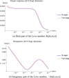 |
Fig. 4 Comparison between the exact five-layer lunar model and the equivalent homogeneous generalized Voigt model. The real and imaginary parts of the tidal Love number coincide within numerical precision when all extracted Voigt elements are retained. |
Acknowledgements
The author would like to thank the anonymous referee for careful reading and constructive comments that improved the manuscript. The author would also like to thank Clodoaldo Ragazzo (USP) for many discussions and long-standing collaboration on this topic, Diogo Gomes and Alessandro Astolfi (KAUST) for their kind support, and J. Ricardo G. Mendonça (USP) for technical advice and a careful reading of the manuscript that greatly improved its presentation. This work was partially supported by the King Abdullah University of Science and Technology (KAUST), Saudi Arabia.
References
- Bierson, C. J., & Nimmo, F. 2016, J. Geophys. Res. (Planets), 121, 2211 [Google Scholar]
- Bolmont, E., Breton, S. N., Tobie, G., et al. 2020, A&A, 644, A165 [NASA ADS] [CrossRef] [EDP Sciences] [Google Scholar]
- de Oliveira, V. M., Ragazzo, C., & Correia, A. C. M. 2025a, A&A, 693, A5 [NASA ADS] [CrossRef] [EDP Sciences] [Google Scholar]
- de Oliveira, V. M., Ragazzo, C., & Correia, A. C. M. 2025b, Astrophysics Source Code Library [record ascl:2508.007] [Google Scholar]
- Gevorgyan, Y. 2021, A&A, 650, A141 [NASA ADS] [CrossRef] [EDP Sciences] [Google Scholar]
- Gevorgyan, Y., Boué, G., Ragazzo, C., Ruiz, L. S., & Correia, A. C. M. 2020, Icarus, 343, 113610 [NASA ADS] [CrossRef] [Google Scholar]
- Gevorgyan, Y., Matsuyama, I., & Ragazzo, C. 2023, MNRAS, 523, 1822 [Google Scholar]
- Hussmann, H., & Spohn, T. 2004, Icarus, 171, 391 [NASA ADS] [CrossRef] [Google Scholar]
- Matsuyama, I., Nimmo, F., Keane, J. T., et al. 2016, Geophys. Res. Lett., 43, 8365 [Google Scholar]
- Sabadini, R., Vermeersen, B., & Cambiotti, G. 2016, Global Dynamics of the Earth (Springer) [Google Scholar]
- Thomas, P. C., Tajeddine, R., Tiscareno, M. S., et al. 2016, Icarus, 264, 37 [NASA ADS] [CrossRef] [Google Scholar]
- Wahr, J. M., Zuber, M. T., Smith, D. E., & Lunine, J. I. 2006, J. Geophys. Res. (Planets), 111, E12005 [Google Scholar]
All Tables
Extracted parameters for the Kelvin–Voigt elements of the full effective lunar model.
Love numbers and effective rheological parameters for the lunar homogeneous model.
All Figures
|
Fig. 1 Schematic representation of the generalized Voigt model. |
| In the text | |
|
Fig. 2 Workflow of the computeHomogeneous pipeline. |
| In the text | |
|
Fig. 3 Cross-section depiction of the five-layer lunar interior model automatically generated by the VisualizeLayers.wl routine. The numbered list indicates the thickness of each corresponding layer, along with the position (radius) of its outer boundary in parentheses. |
| In the text | |
|
Fig. 4 Comparison between the exact five-layer lunar model and the equivalent homogeneous generalized Voigt model. The real and imaginary parts of the tidal Love number coincide within numerical precision when all extracted Voigt elements are retained. |
| In the text | |
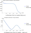 |
Fig. 5 Same as Fig. 4, but for the reduced equivalent homogeneous generalized Voigt model. |
| In the text | |
Current usage metrics show cumulative count of Article Views (full-text article views including HTML views, PDF and ePub downloads, according to the available data) and Abstracts Views on Vision4Press platform.
Data correspond to usage on the plateform after 2015. The current usage metrics is available 48-96 hours after online publication and is updated daily on week days.
Initial download of the metrics may take a while.