| Issue |
A&A
Volume 710, June 2026
|
|
|---|---|---|
| Article Number | L19 | |
| Number of page(s) | 5 | |
| Section | Letters to the Editor | |
| DOI | https://doi.org/10.1051/0004-6361/202660495 | |
| Published online | 12 June 2026 | |
Letter to the Editor
Understanding hydrodynamical wave-driven shear mixing in stellar radiation zones
Looking in the mirror of the dyapicnal oceanic mixing
Université Paris-Saclay, Université Paris Cité, CEA, CNRS, AIM, F-91191 Gif-sur-Yvette, France
★ Corresponding author: This email address is being protected from spambots. You need JavaScript enabled to view it.
Received:
19
April
2026
Accepted:
18
May
2026
Abstract
Context. Stellar radiation zones play a key role in the long-term magneto-rotational and chemical evolution of stars and of their planetary and galactic neighborhoods. Similarly to parts of the atmosphere and oceans of the Earth, they are stably stratified and rotating. Therefore, their dynamics is controlled by the Archimedean buoyancy force and the Coriolis acceleration. Asteroseismology and high-resolution spectroscopy have showed that they are the seat of an efficient extraction of angular momentum and of a mild mixing of chemicals that must be more fully understood. In this context, particle tracing in recent non-linear hydrodynamical equatorial numerical simulations of stellar radiation zones, where internal gravity waves (IGWs) are propagating, has led to the measurement of an effective diffusivity following the prescriptions derived by Garcia-Lopez & Spruit and by Zahn for the inflectional instability of the vertical shear of low-frequency IGWs. However, the associated instability criteria have not been fulfilled. This effective diffusivity is found to scale as the squared velocity of IGWs for every rotation rates. Other dependencies have also been derived in the literature as, for instance, in the case of the Stokes displacement.
Aims. We aim to provide a physical interpretation of these phenomena.
Methods. To reach this objective, we propose exploring the parameterisation for the mixing of particles, which has been proposed in another rotating stably stratified systems: the oceans of Earth. A foundation stone in physical oceanography is the so-called Osborn & Cox energetic balance that leads to an effective dyapicnal diffusivity for the transport of matter that scales as the ratio of the dissipation of the fluctuating flows over the squared Brunt-Väisälä stratification frequency. We applied this parameterisation for the mixing to the field of low-frequency IGWs propagating in stellar radiation zones.
Results. We demonstrate that the effective dyapicnal diffusivity, widely used in modeling the oceanic general circulation, is equivalent to the eddy diffusivity derived by Zahn for the inflectional instability of the vertical shear applied to low-frequency IGWs. This allows us to characterise the corresponding energetic balance where the power extracted by the waves from the mean flows is balanced by their dissipation and by the power produced by their buoyancy flux for any rotation rate. This bridge established between results obtained across geophysical and stellar fluid dynamics illustrates the high interest of a cross-fertilisation between these research fields when we are aiming to evaluate and robustly model the effects of small-scale and short-timescale phenomena such as IGWs on the long-term evolution of large-scale oceanic, atmospheric, and stellar general circulation processes.
Key words: waves / methods: analytical / planets and satellites: atmospheres / planets and satellites: oceans / stars: evolution / stars: rotation
© The Authors 2026
 Open Access article, published by EDP Sciences, under the terms of the Creative Commons Attribution License (https://creativecommons.org/licenses/by/4.0), which permits unrestricted use, distribution, and reproduction in any medium, provided the original work is properly cited.
This article is published in open access under the Subscribe to Open model. This email address is being protected from spambots. You need JavaScript enabled to view it. to support open access publication.
1. Introduction
In a standard vision of stellar structure and evolution, stably stratified stellar radiation zones are assumed to be in hydrostatic and radiative balances, while serving as the seat of microscopic mixing processes. However, space-based seismology of our Sun and other stars has revealed that they are the seat of strong transport processes of angular momentum and the mild macroscopic mixing of chemicals (e.g. Pinsonneault 1997; Aerts et al. 2019; Christensen-Dalsgaard 2021; Aerts & Tkachenko 2024). These mechanisms have a strong impact on the evolution of stars; for instance, on their age and on their chemical properties. In addition, at the largest scales, they impact galactic evolution (Maeder 2009). Several mechanisms have been identified as serious candidates to simultaneously reproduce the rotation probed by helio- and asteroseismology at different depths in our Sun and stars, respectively, and their chemical composition. To start, the hydrodynamical instabilities of the differential rotation have been studied (Zahn 1983; Prat & Lignières 2014; Park et al. 2021; Dymott et al. 2023; Garaud et al. 2024; Park & Mathis 2025) in combination with the meridional circulation they trigger with angular momentum losses at the stellar surface (Zahn 1992; Maeder & Zahn 1998; Mathis & Zahn 2004). This so-called type-I rotational mixing has demonstrated success in explaining the observed chemical abundances in massive stars (Maeder & Meynet 2000), but failed to explain the strong extraction of angular momentum observed in the Sun and in stars of different masses at different evolutionary stages (Turck-Chièze et al. 2010; Marques et al. 2013; Ouazzani et al. 2019). Furthermore, magnetic fields and their instabilities (Spruit 1999, 2002; Mathis & Zahn 2005; Barrère et al. 2026) and low-frequency IGWs excited by the turbulence at the interfaces with adjacent convective regions and in their bulk (e.g. Press 1981; Schatzman 1993; Zahn et al. 1997; Fuller et al. 2014; Rogers 2015; Pinçon et al. 2017) have been examined; this is the so-called type-II rotational mixing. Both mechanisms have demonstrated their potential ability to reproduce solar and stellar rotational and chemical properties (we refer to Eggenberger et al. 2005 and Eggenberger et al. 2022 in the case of magnetic fields and Charbonnel & Talon 2005 and Talon & Charbonnel 2005 in the case of IGWs). In particular, IGWs can be an efficient and discriminant vector of chemical mixing of light elements in late-type stars (Montalbán & Schatzman 2000; Charbonnel & Talon 2005), evolved stars (Denissenkov & Tout 2003), and early-type stars (Herwig et al. 2023; Mombarg et al. 2025).
In this context, Rogers & McElwaine (2017) computed non-linear hydrodynamical equatorial simulations of a 3 M⊙ star, which simultaneously computes the dynamics of its convective core and its radiative envelope. Using a particle tracer method, they show that IGWs act as an effective diffusion for the concentration of chemicals and that the associated eddy-diffusion scales as the squared velocity of IGWs. These results have been confirmed in a subsequent series of articles (Varghese et al. 2023, 2024), where different stellar masses, evolutionary stages and rotation were taken into consideration and examined. While these results have been debated by Morton et al. (2025), the paper by Varghese et al. (2025) consolidated and confirmed these findings, demonstrating that the functional dependence of the diffusion coefficient as a function of the velocity of IGWs can be explained by their own vertical shear instabilities. However, two questions remain open. On the one hand, IGWs observed in the work of Varghese et al. (2025) do not fullfill the vertical shear instability criterion. On the other hand, other functional dependences of the diffusion have been proposed in the literature. For instance, it scales as the fourth power of the velocity of IGWs if we assume the diffusion is due to the so-called Stokes displacement induced by the thermal dissipation of IGWs.
To try and address these two questions in this work, we propose exploiting the similarities among stellar radiation zones with terrestrial oceans. Both systems are the seat of a complex field of propagative IGWs excited at their boundaries: via adjacent turbulent convective regions and potential planetary companions in stars (e.g. Zahn 1975; Barker & Ogilvie 2010; Ahuir et al. 2021) as well as by the winds, topography, and the solar and lunar tides in the oceans, as illustrated in Fig. 1. In the oceanic case, an important store of literature has been developed since the seminal work by Osborn & Cox (1972) and Osborn (1980) to evaluate the mixing triggered by small scale and short-timescale fluctuating flows, possibly including progressive IGWs. In addition, there is the related effective diffusivity, which has been used as a parameterisation in oceanic global circulation models (e.g. MacKinnon et al. 2017, and references therein). We recall in Sect. 2 the details of the physical basis of the Osborn & Cox model and the related diffusion parameterisation. We show in Sect. 3 how it can be applied to the stellar case, thereby allowing us to provide a complementary understanding of the results obtained recently in the literature. Finally, in Sect. 4 we discuss plans for future developments and we present our conclusions.
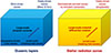 |
Fig. 1. Analogies between stably stratified rotating oceanic layers and stellar (planetary) radiation zones. In both cases, internal gravity and gravito-inertial waves are excited in the adjacent convective layers, by the topography in the case of the Earth, and by tides exerted by the Sun and the Moon in the case of the Earth as well as those induced by planetary or stellar companions in the astrophysical context. |
2. The Osborn-Cox closure model
In their work, Osborn & Cox (1972) and Osborn (1980) have proposed a closure model to parameterise and evaluate the mixing in rotating stably stratified oceanic layers. They split the components of the velocity and thermodynamical quantities following
 (1)
(1)
where  and ⋅ ⋅ ⋅′ are their mean and fluctuating components, respectively. Next, they considered the Reynolds equation for the fluctuating components,
 (2)
(2)
which are the mean kinetic energy of the fluctuating components of the velocity and their viscous energy dissipation with the viscosity, ν, respectively. We considered fluctuating velocities and perturbations that vary over small characteristic length-scales when compared to those of the variations of the hydrostatic background. This allows us to assume the Boussinesq approximation and we can introduce ρB the corresponding constant and uniform reference density. We introduce the Lagrangian derivative  and the stress tensor as
 (3)
(3)
When assuming a statistical steady state and that the first three redistribution flux terms on the right-hand side of Eq. (2) can be neglected in front of the three last terms, Osborn & Cox (1972) and Osborn (1980) identified the balance between the power transferred from the mean flow to the fluctuating velocities, their viscous dissipation, and the power of their buoyancy flux,
 (4)
(4)
Next, they evaluated the transport of mass using an effective dyapicnal eddy diffusivity and the flux Richardson number that they defined as
 (5)
(5)
This latter measures the fraction of fluctuating (turbulent) power generated by the mean shear that is converted into mixing against the stabilising stratification term. These follow from Eq. (4) via
 (6)
(6)
which is an efficiency parameter associated with possible mixing processes that increases with Rf. Following the path proposed by Osborn & Cox, Hamilton et al. (1989) demonstrated that this relationship can also be applied to other fluctuating thermodynamical quantities,
 (7)
(7)
where X ≡ {T,S} with T and S as the temperature and the oceanic salinity (the mean molecular weight in an astrophysical body), respectively (we refer the reader to Hamilton et al. 1989, for the detailed derivation of the efficiency parameters ΓX as a function of Γρ and of thermodynamical quantities). This parameterisation has been widely used in oceanic general circulation models (MacKinnon et al. 2017). Since this parameterisation is aimed at describing the mixing of chemicals in oceanic rotating stably stratified layers, its application to the astrophysical context of stellar (and planetary) rotating stably stratified radiation zones is of key interest.
3. Recovering the prescription for the wave vertical shear-driven mixing in stellar radiation zones
3.1. The effective diffusivity
We considered a (rotating) stably stratified stellar radiation zone. In such a region, the buoyancy restoring force is limiting the motion along the radial direction of the entropy and chemical stratifications. In the case of low-frequency internal (gravito-inertial) gravity waves, which are efficient to transport momentum and matter (e.g. Press 1981; Schatzman 1993; Zahn et al. 1997; Mathis et al. 2008), this leads to ur ≪ uh, where ur and uh are the radial and horizontal components of their velocity, respectively. Considering the Osborn-Cox prescription given in Eq. (7), we can obtain an approximation of the energy dissipation via
 (8)
(8)
Assuming that the fluctuating motions, which are considered in the Osborn-Cox modelling, can be low-frequency internal gravito-inertial or gravity waves, we thus obtain for the eddy-like diffusion coefficient of a passive scalar the form
 (9)
(9)
where we introduce  , where Pr = ν/K is the Prandtl number, which evaluates the relative strength of the viscosity and of the heat diffusivity, K (in stellar radiation zones Pr < 1 while Pr ∼ 7 in oceans). This straightforward result is of high interest since we were able to recover the Zahn (1992) prescription applied to the vertical shear of low-frequency internal waves (Varghese et al. 2025), first derived by Garcia Lopez & Spruit (1991). Recently, Varghese et al. (2025) robustly demonstrated numerically that the transport of chemicals by internal waves they observed in their series of non-linear hydrodynamical equatorial numerical simulations of non-rotating and rotating early-type and late-type stars can be modeled with such a functional dependence.
If, again, we take advantage of the fact that low-frequency internal waves are rapidly oscillating along the radial direction and that these dependence can be described using the JWKB asymptotic approximation where |∂ruh|∼kr|uh|, with kr being the radial component of the wave vector, we see that DX ∝ |uh|2. This dependence was first identified by Rogers & McElwaine (2017) in their similar numerical simulations of a 3 M⊙ star. Next, it was confirmed by Varghese et al. (2023), who studied different stellar masses and evolutionary stages, as well as by Varghese et al. (2024), who examined the dependence as a function of stellar rotation. In this regime, the vertical dependence of the horizontal component of the velocity of the waves can be expressed using the JWKB approximation (e.g. Mathis 2025) and we get
![Mathematical equation: $$ \begin{aligned}&{u}_{h}\left(r,X_h,t\right) = {\widehat{u}}_{h}\left(r_0,\omega \right)\times \nonumber \\&\quad \left(\frac{\epsilon \left(r\right)}{\epsilon \left(r_0\right)}\right){\mathcal{H} }\left(X_{h}\right)\exp \left[i\,\left(\pm \int _{r_0}^{r}k_r\left(r\prime \right){\mathrm{d} r\prime }+\omega t\right)\right], \end{aligned} $$](/articles/aa/full_html/2026/06/aa60495-26/aa60495-26-eq13.gif) (10)
(10)
where r0 is the radius of their excitation region, ϵ(r) their slowly varying JWKB envelope, which can include their linear damping, Xh a generic horizontal coordinate adapted to the studied geometry, and  the corresponding function describing the horizontal variations of the waves (noting that we refer to the Appendix A for their explicit expressions in the different used geometries), ω their angular frequency, and t the time. The effective diffusivity becomes
![Mathematical equation: $$ \begin{aligned} D_{\rm X}=\frac{1}{2}{\widetilde{\Gamma }}_{X}\frac{K}{N^2}\left[k_r\left(r\right)\frac{\epsilon \left(r\right)}{\epsilon \left(r_0\right)}{\widehat{u}}_{h}\left(r_0,\omega \right)\right]^2 \left < {\mathcal{H} }\left(X_{h}\right)\left[{\mathcal{H} }\left(X_{h}\right)\right]^{*}\right>_{h}, \end{aligned} $$](/articles/aa/full_html/2026/06/aa60495-26/aa60495-26-eq15.gif) (11)
(11)
where  is the average over the horizontal directions in the considered geometry and * the complex conjugate.
A key concern at this point is to find out if low-frequency internal waves can legitimately be considered as the fluctuating field in the Osborn-Cox methodology when applied to stellar radiation zones. We think that a positive answer can be assumed. On the one hand, low-frequency internal waves have very short radial wavelengths when compared to the characteristic lengths of variation of the hydrostatic stellar gravity and thermodynamical quantities (i.e. density, entropy, temperature, and mean molecular weight) and of the differential rotation. On the other hand, low-frequency internal waves have characteristic periods that are very short when compared to the characteristic times of the secular extraction or deposit of angular momentum they trigger (we refer the reader to the detailed discussion in Talon & Charbonnel 2005). To assume such an hypothesis, we assume that the interactions occurring between the waves and the differential rotation (and the associated mean zonal velocity) such as the so-called quasi-biennal oscillation observed in the equatorial region of the terrestrial atmosphere (e.g. Baldwin et al. 2001) and its stellar analog, the so-called shear layer oscillation (e.g. Talon & Charbonnel 2005), are filtered out. Finally, it should be underlined, as pointed out by Osborn (1980), that when shear instabilities set up, it can be difficult to disentangle fluctuating turbulent flows from wave motions (Alvan et al. 2013; Herbert et al. 2016; Lam et al. 2021).
3.2. Impact of the Coriolis acceleration
Another interesting point concerning the Osborn-Cox balance is that it has been derived with taking into account the Coriolis acceleration in the initial momentum equations. As a consequence, the related effective diffusivity can be applied to the vertical shear of low-frequency internal gravity and gravito-inertial waves. This result is coherent with the results obtained by Varghese et al. (2025), where the measured effective diffusivity scales as in Eq. (11) independently of the rotation rate. This is also in agreement with the theoretical results obtained by Park & Mathis (2025), where we showed that the inflectional instability of vertically sheared flows (here, the horizontal velocity of low-frequency internal gravity and gravito-inertial waves) is only weakly directly influenced by the Coriolis acceleration. Such a weak dependence has also been observed in non-linear hydrodynamical equatorial simulations computed by Chang & Garaud (2021).
4. Discussion and conclusions
In this Letter, we examine the recent results obtained on the mixing of chemicals in stably-stratified rotating stellar radiation zones using the so-called Osborn-Cox closure model (Osborn & Cox 1972; Osborn 1980), which is widely used in physical oceanography. This model splits flows into mean and fluctuating components in stably stratified rotating oceanic layers and proposes a parameterisation of the mass transport (i.e. dyapicnal mixing) by an effective eddy-like diffusion for the density, entropy, temperature, and chemical composition (Hamilton et al. 1989). Assuming that the fluctuating velocity field in stellar radiation zones is composed of low-frequency progressive internal gravity and gravito-inertial waves, the Osborn-Cox closure model leads to an effective eddy-like diffusion for the chemicals they transport. This is scaled as the ratio of the product of the heat diffusivity multiplied by the squared vertical shear of the horizontal component of their velocity divided by the squared Brunt-Väsälä frequency. This result is of key interest, since this effective diffusion with such dependencies has been measured in state-of-the-art non-linear hydrodynamical equatorial numerical simulations computed by Varghese et al. (2025) for early-type and late-type stars at different rotation rates (we refer also the reader to Rogers & McElwaine 2017; Varghese et al. 2023, 2024). Therefore, we obtain a complementary physical understanding of this measured effective diffusivity by showing that it is associated to a balance between the power transferred from the mean flow to the fluctuating velocities, their energy dissipation, and the power of their buoyancy flux that leads to mixing. This balance has been derived from the Navier-Stokes equations while simultaneously taking into account the buoyancy force and the Coriolis acceleration. Therefore, this parameterisation can be applied both to internal gravity waves (e.g. Zahn et al. 1997; Mathis 2025) and to gravito-inertial waves (e.g. Mathis et al. 2008; Mathis 2009; Varghese et al. 2024; Mathis 2026) in any rotating star along its evolution. This strengthens the interest of its implementation both for existing 1D and in forthcoming multi-D stellar structure and evolution models (e.g. Talon & Charbonnel 2005; Mombarg et al. 2025).
However, this work does not close the quest for parameterisations of wave-driven mixing. Indeed, this type of mixing could be driven by other mechanisms such as the irreversible Stokes displacement (e.g. Press 1981; Schatzman 1993; Mao & Lecoanet 2025) or the wave convective and shear-induced breaking (Lindzen 1981; Liu et al. 2025) with possible couplings of the different instabilities of the waves (e.g. Lombard & Riley 1996; Howland et al. 2021). Therefore, our long-term goal is to provide coherent parameterisations for every possible physical configuration.
Acknowledgments
S.M. warmly thanks the anonymous referee for their constructive suggestions, which have allowed to improve the article. He also acknowledges support from the European Research Council (ERC) under the Horizon Europe programme (Synergy Grant agreement 101071505: 4D-STAR), from the CNES SOHO-GOLF and PLATO grants at CEA-DAp, and from PNPS (CNRS/INSU). While partially funded by the European Union, views and opinions expressed are however those of the author only and do not necessarily reflect those of the European Union or the European Research Council. Neither the European Union nor the granting authority can be held responsible for them.
References
- Aerts, C., & Tkachenko, A. 2024, A&A, 692, R1 [NASA ADS] [CrossRef] [EDP Sciences] [Google Scholar]
- Aerts, C., Mathis, S., & Rogers, T. M. 2019, ARA&A, 57, 35 [Google Scholar]
- Ahuir, J., Mathis, S., & Amard, L. 2021, A&A, 651, A3 [NASA ADS] [CrossRef] [EDP Sciences] [Google Scholar]
- Alvan, L., Mathis, S., & Decressin, T. 2013, A&A, 553, A86 [CrossRef] [EDP Sciences] [Google Scholar]
- Baldwin, M. P., Gray, L. J., Dunkerton, T. J., et al. 2001, Rev. Geophys., 39, 179 [CrossRef] [Google Scholar]
- Barker, A. J., & Ogilvie, G. I. 2010, MNRAS, 404, 1849 [NASA ADS] [Google Scholar]
- Barrère, P., Guilet, J., Gallet, B., & Raynaud, R. 2026, arXiv e-prints [arXiv:2601.02182] [Google Scholar]
- Chang, E., & Garaud, P. 2021, MNRAS, 506, 4914 [Google Scholar]
- Charbonnel, C., & Talon, S. 2005, Science, 309, 2189 [Google Scholar]
- Christensen-Dalsgaard, J. 2021, Liv. Rev. Sol. Phys., 18, 2 [NASA ADS] [CrossRef] [Google Scholar]
- Denissenkov, P. A., & Tout, C. A. 2003, MNRAS, 340, 722 [NASA ADS] [CrossRef] [Google Scholar]
- Dymott, R. W., Barker, A. J., Jones, C. A., & Tobias, S. M. 2023, MNRAS, 524, 2857 [Google Scholar]
- Eggenberger, P., Maeder, A., & Meynet, G. 2005, A&A, 440, L9 [NASA ADS] [CrossRef] [EDP Sciences] [Google Scholar]
- Eggenberger, P., Buldgen, G., Salmon, S. J. A. J., et al. 2022, Nat. Astron., 6, 788 [NASA ADS] [CrossRef] [Google Scholar]
- Fuller, J., Lecoanet, D., Cantiello, M., & Brown, B. 2014, ApJ, 796, 17 [Google Scholar]
- Garaud, P., Khan, S., & Brown, J. M. 2024, ApJ, 961, 220 [Google Scholar]
- Garcia Lopez, R. J., & Spruit, H. C. 1991, ApJ, 377, 268 [NASA ADS] [CrossRef] [Google Scholar]
- Gerkema, T., & Shrira, V. I. 2005, J. Fluid Mech., 529, 195 [Google Scholar]
- Hamilton, J. M., Lewis, M. R., & Ruddick, B. R. 1989, J. Geophys. Res., 94, 2137 [Google Scholar]
- Herbert, C., Marino, R., Rosenberg, D., & Pouquet, A. 2016, J. Fluid Mech., 806, 165 [Google Scholar]
- Herwig, F., Woodward, P. R., Mao, H., et al. 2023, MNRAS, 525, 1601 [NASA ADS] [CrossRef] [Google Scholar]
- Howland, C. J., Taylor, J. R., & Caulfield, C. P. 2021, J. Fluid Mech., 921, A24 [Google Scholar]
- Lam, H., Delache, A., & Godeferd, F. S. 2021, J. Fluid Mech., 923, A31 [Google Scholar]
- Lindzen, R. S. 1981, J. Geophys. Res., 86, 9707 [NASA ADS] [CrossRef] [Google Scholar]
- Liu, J., Millour, E., Forget, F., Lott, F., & Chaufray, J.-Y. 2025, J. Geophys. Res. (Planets), 130, e2025JE009188 [Google Scholar]
- Lombard, P. N., & Riley, J. J. 1996, Phys. Fluids, 8, 3271 [Google Scholar]
- MacKinnon, J. A., Zhao, Z., Whalen, C. B., et al. 2017, Bull. Am. Meteorol. Soc., 98, 2429 [Google Scholar]
- Maeder, A. 2009, Physics, Formation and Evolution of Rotating Stars (Springer) [Google Scholar]
- Maeder, A., & Meynet, G. 2000, ARA&A, 38, 143 [Google Scholar]
- Maeder, A., & Zahn, J.-P. 1998, A&A, 334, 1000 [NASA ADS] [Google Scholar]
- Mao, Y., & Lecoanet, D. 2025, arXiv e-prints [arXiv:2510.02031] [Google Scholar]
- Marques, J. P., Goupil, M. J., Lebreton, Y., et al. 2013, A&A, 549, A74 [NASA ADS] [CrossRef] [EDP Sciences] [Google Scholar]
- Mathis, S. 2009, A&A, 506, 811 [CrossRef] [EDP Sciences] [Google Scholar]
- Mathis, S. 2025, A&A, 694, A173 [NASA ADS] [CrossRef] [EDP Sciences] [Google Scholar]
- Mathis, S. 2026, A&A, 706, A71 [NASA ADS] [CrossRef] [EDP Sciences] [Google Scholar]
- Mathis, S., & Zahn, J.-P. 2004, A&A, 425, 229 [NASA ADS] [CrossRef] [EDP Sciences] [Google Scholar]
- Mathis, S., & Zahn, J.-P. 2005, A&A, 440, 653 [NASA ADS] [CrossRef] [EDP Sciences] [Google Scholar]
- Mathis, S., Talon, S., Pantillon, F.-P., & Zahn, J.-P. 2008, Sol. Phys., 251, 101 [Google Scholar]
- Mombarg, J. S. G., Varghese, A., & Ratnasingam, R. P. 2025, A&A, 695, A255 [NASA ADS] [CrossRef] [EDP Sciences] [Google Scholar]
- Montalbán, J., & Schatzman, E. 2000, A&A, 354, 943 [Google Scholar]
- Morton, J., Guillet, T., Baraffe, I., et al. 2025, MNRAS, 537, 154 [Google Scholar]
- Osborn, T. R. 1980, J. Phys. Oceanogr., 10, 83 [Google Scholar]
- Osborn, T. R., & Cox, C. S. 1972, Geophys. Fluid Dyn., 3, 321 [Google Scholar]
- Ouazzani, R.-M., Marques, J. P., Goupil, M.-J., et al. 2019, A&A, 626, A121 [NASA ADS] [CrossRef] [EDP Sciences] [Google Scholar]
- Park, J., & Mathis, S. 2025, MNRAS, 540, 298 [Google Scholar]
- Park, J., Prat, V., Mathis, S., & Bugnet, L. 2021, A&A, 646, A64 [EDP Sciences] [Google Scholar]
- Pinçon, C., Belkacem, K., Goupil, M. J., & Marques, J. P. 2017, A&A, 605, A31 [NASA ADS] [CrossRef] [EDP Sciences] [Google Scholar]
- Pinsonneault, M. 1997, ARA&A, 35, 557 [NASA ADS] [CrossRef] [Google Scholar]
- Prat, V., & Lignières, F. 2014, A&A, 566, A110 [NASA ADS] [CrossRef] [EDP Sciences] [Google Scholar]
- Press, W. H. 1981, ApJ, 245, 286 [Google Scholar]
- Rogers, T. M. 2015, ApJ, 815, L30 [Google Scholar]
- Rogers, T. M., & McElwaine, J. N. 2017, ApJ, 848, L1 [CrossRef] [Google Scholar]
- Schatzman, E. 1993, A&A, 279, 431 [NASA ADS] [Google Scholar]
- Spruit, H. C. 1999, A&A, 349, 189 [NASA ADS] [Google Scholar]
- Spruit, H. C. 2002, A&A, 381, 923 [CrossRef] [EDP Sciences] [Google Scholar]
- Talon, S., & Charbonnel, C. 2005, A&A, 440, 981 [NASA ADS] [CrossRef] [EDP Sciences] [Google Scholar]
- Turck-Chièze, S., Palacios, A., Marques, J. P., & Nghiem, P. A. P. 2010, ApJ, 715, 1539 [Google Scholar]
- Varghese, A., Ratnasingam, R. P., Vanon, R., Edelmann, P. V. F., & Rogers, T. M. 2023, ApJ, 942, 53 [NASA ADS] [CrossRef] [Google Scholar]
- Varghese, A., Ratnasingam, R. P., Vanon, R., et al. 2024, ApJ, 970, 104 [Google Scholar]
- Varghese, A., Ratnasingam, R. P., Ramírez-Galeano, L., Mathis, S., & Rogers, T. M. 2025, ApJ, 992, L5 [Google Scholar]
- Zahn, J.-P. 1975, A&A, 41, 329 [Google Scholar]
- Zahn, J. P. 1983, in Saas-Fee Advanced Course 13: Astrophysical Processes in Upper Main Sequence Star, eds. A. N. Cox, S. Vauclair, & J. P. Zahn, 253 [Google Scholar]
- Zahn, J.-P. 1992, A&A, 265, 115 [NASA ADS] [Google Scholar]
- Zahn, J.-P., Talon, S., & Matias, J. 1997, A&A, 322, 320 [Google Scholar]
Appendix A: Explicit expressions for the different geometries
In Cartesian coordinates in Mathis (2026), Xh = χ, the reduced horizontal coordinate introduced by Gerkema & Shrira (2005), ![Mathematical equation: $ \mathcal{H}\left(X_{h}\right)\equiv\exp\left[i k_{\perp} \chi\right] $](/articles/aa/full_html/2026/06/aa60495-26/aa60495-26-eq17.gif) , and
, and ![Mathematical equation: $ \epsilon\left(r\right) = \left[k_{r}\left(r\right)\right]^{-1/2}\left[k_{r}\left(r\right)/k_{\perp}\right]\left[\left(f^2+{\widehat\omega}^2\right)/{\widehat\omega}^2\right]^{1/2} $](/articles/aa/full_html/2026/06/aa60495-26/aa60495-26-eq18.gif) , where kr is given by their Eq. (15), f = 2Ω cos θ with Ω the angular velocity and θ the co-latitude, and
, where kr is given by their Eq. (15), f = 2Ω cos θ with Ω the angular velocity and θ the co-latitude, and  the wave’s Doppler-shifted frequency.
In polar coordinates in Varghese et al. (2024), Xh ≡ ϕ the polar angle, ![Mathematical equation: $ \mathcal{H}\left(X_{h}\right)\equiv\exp\left[i m \phi\right] $](/articles/aa/full_html/2026/06/aa60495-26/aa60495-26-eq20.gif) , and
, and ![Mathematical equation: $ \epsilon\left(r\right) = {\overline\rho}^{\,-1/2}r^{-3/2}\left[k_{r}\left(r\right)\right]^{-1/2}\left[k_{r}\left(r\right)/k_{h}\left(r\right)\right] $](/articles/aa/full_html/2026/06/aa60495-26/aa60495-26-eq21.gif) , where
, where  with kh ≡ m/r, where m is the azimuthal degree.
In spherical coordinates, Xh ≡ {θ,φ}, the colatitude and the azimuth, respectively,  the usual spherical harmonics, and
 ![Mathematical equation: $ \epsilon\left(r\right) = {\overline\rho}^{\,-1/2}r^{-2}\left[k_{r}\left(r\right)\right]^{-1/2}\left[k_{r}\left(r\right)/k_{h}\left(r\right)\right] $](/articles/aa/full_html/2026/06/aa60495-26/aa60495-26-eq24.gif) , where
, where  with
with  .
.
Note that the Coriolis acceleration can be taken into account using the Traditional Approximation of Rotation if 2Ω ≪ N (e.g. Mathis et al. 2008). In this case the spherical harmonics can be replaced by the so-called Hough functions as well as their horizontal eigenvalues.
All Figures
|
Fig. 1. Analogies between stably stratified rotating oceanic layers and stellar (planetary) radiation zones. In both cases, internal gravity and gravito-inertial waves are excited in the adjacent convective layers, by the topography in the case of the Earth, and by tides exerted by the Sun and the Moon in the case of the Earth as well as those induced by planetary or stellar companions in the astrophysical context. |
| In the text | |
Current usage metrics show cumulative count of Article Views (full-text article views including HTML views, PDF and ePub downloads, according to the available data) and Abstracts Views on Vision4Press platform.
Data correspond to usage on the plateform after 2015. The current usage metrics is available 48-96 hours after online publication and is updated daily on week days.
Initial download of the metrics may take a while.