| Issue |
A&A
Volume 547, November 2012
|
|
|---|---|---|
| Article Number | A46 | |
| Number of page(s) | 20 | |
| Section | The Sun | |
| DOI | https://doi.org/10.1051/0004-6361/201219477 | |
| Published online | 24 October 2012 | |
Online material
Appendix A: Formal solution: influence of the source function interpolation method
In the short characteristics (SC) method (Olson & Kunasz 1987; Kunasz & Auer 1988), the formal solution is integrated only along the “short” path from the nearest up- and downwind points. The incoming intensities – as well as all other quantities used for the formal integration at the up- and downwind points – have usually to be interpolated from neighboring grid points. The problem of polynomial interpolation at the up- and downwind points, which may lead to spurious extrema, was widely discussed in the literature until Auer & Paletou (1994) found an elegant and efficient solution using monotonic interpolation.
In contrast, one finds very few references to the problems that arise when the source
function is interpolated with a parabolic Lagrange polynomial along the short
characteristic as proposed and established as standard by Auer et al. (1994). With
S(τ) = S0 + c1τ + c2τ2,
the integral over S along the short characteristics is then given by
the analytical expression  (A.1)where
Ilocal is the locally produced intensity without
irradiation from outside. The wi may be –
in the case of Lagrange interpolation – expressed as simple functions of known
quantities (see Auer & Paletou 1994). The
first indication of these interpolation problems is given by Auer (2003), who proposes monotonic Bézier interpolation instead of
simple Lagrange interpolation to prevent spurious extrema of S along
the integration path.
(A.1)where
Ilocal is the locally produced intensity without
irradiation from outside. The wi may be –
in the case of Lagrange interpolation – expressed as simple functions of known
quantities (see Auer & Paletou 1994). The
first indication of these interpolation problems is given by Auer (2003), who proposes monotonic Bézier interpolation instead of
simple Lagrange interpolation to prevent spurious extrema of S along
the integration path.
To demonstrate that the proper interpolation of S is as important as
the correct interpolation of up- and downwind quantities, we present the situation of an
overshooting source function, which we call “a critical case”, taken from our fluxsheet
atmosphere simulation (the standard model, see Sect. 2.3 for a description). Figure A.1 shows
the values of S at the up- and downwind
points (S1, S2)
and the integration point (S0). The unique Lagrange parabola
through the three base points is given by the solid line. One immediately sees
that S clearly takes values below the base
points S0 and S1, while it
should decrease monotonically from S0
to S1. From  (A.2)it directly
follows that the resulting intensity must be wrong (i.e. too small), because the area
under S is far too small. We note that the
factor e−τ does not change the qualitative result as
it is on the order of unity over the relevant integration interval.
(A.2)it directly
follows that the resulting intensity must be wrong (i.e. too small), because the area
under S is far too small. We note that the
factor e−τ does not change the qualitative result as
it is on the order of unity over the relevant integration interval.
 |
Fig. A.1
Interpolation methods: the Lagrange parabola (solid) does not give a good representation of the run of S along the short characteristic from S0 to S1. Parabolic monotonic Bézier interpolation (dashed) is achieved by restricting the control point c0 (defined by the two tangents (dotted) of each parabola) to S0 < = c′0 < = S1. |
| Open with DEXTER | |
Bézier parabolas are defined by two base point values and a single control point, which is always located at the intersection of the two tangents of S at the base points. This control point therefore “controls” the run of S between the two base points. The unique Lagrange parabola through S0, S1, and S2 is recovered in the interval from S0 to S1 when the control point (c0 in Fig. A.1) lies on the corresponding tangents of the Lagrange parabola (fine dotted). One imposes monotonicity in the interval from S0 to S1 by constraining the control point to values between the two base point values of S. By moving the control point up to the lower of the two values (c′0), one gets a new parabola (that no longer passes through S2!) with a monotonic run in the integration interval (dashed curve). Therefore, the area under S is no longer artificially reduced. The difference in the locally produced intensity for our sample, taken from an existing calculation, is considerable.
We therefore used monotonic parabolic Bézier interpolation as proposed by Auer (2003) for all our calculations. We performed tests with a snapshot taken from a realistic 3D radiation hydrodynamic simulation run (i.e. for B = 0) with the MURAM code (Vögler et al. 2005). Additionally, we used a 3D version of the FAL-C model of Fontenla et al. (1993) obtained by arranging many identical 1D atmospheres into a 3D cube. In both cases, we found that about 3% of all formal solutions suffer from S overshooting in the integration interval. While the resulting intensity for the FAL-C model is almost the same as for the Lagrange interpolation (most of the critical cases in FAL-C display only quite weak overshooting because of the smoothness of the atmosphere), the resulting intensities in the snapshot may differ considerably owing to the strongly varying atmospheric parameters along the integration path. Therefore, the source function may exhibit strong overshooting.
An increasing number of publications have recognized this problem in recent years. For instance, Hauschildt & Baron (2006) used linear interpolation (instead of monotonic Bézier) for critical cases and Koesterke et al. (2008), and Hayek (2008) used cubic Bézier polynomials.
In more extreme atmospheres than our fluxsheet model (as found e.g. in realistic MHD simulations, which will be discussed in future publications), the resulting intensity may even be wrong by orders of magnitude with disastrous consequences not only for the final result, but also for the convergence of the RT computations themselves. The convergence is affected because the (usually diagonal) approximate Lambda operator used for the improvement of the iteration is generally interpolated in the same manner as the source function.
In our experience, we have found that the monotonic, parabolic Bézier interpolation, which is identical to Lagrange interpolation when S does not overshoot in the integration interval, has much better convergence properties than the pure Lagrange interpolation, which can lead to a complete divergence for non-smooth atmospheres, such as those along rays passing through the walls of a flux tube.
However, imposing either monotonicity or a special treatment in critical cases may lead to convergence problems as well because a change in the interpolation method at a certain point in the cube may influence neighboring points in such a way, that in the next iteration the interpolation method is changed back again to the original method. This may lead to an infinite flip-flop situation, so that convergence is never achieved. We encountered these flip-flop situations in a few of our unsmoothed flux-sheet models. They occurred at a convergence level of a few percent in the population numbers and were much stronger when linear interpolation was used in the critical cases (a change from linear to parabolic may have more influence on the area under S than a change from monotonic Bézier to normal Lagrange parabolas).
The problem of strongly overshooting source functions may also arise in the 1D schemes as they interpolate S in the integration interval with a Lagrange polynomial as well. In addition, we therefore implemented and used monotonic Bézier interpolation for our 1D calculations.
Appendix B: Formal solution for the full Stokes vector problem
 |
Fig. B.1
Interpolation method for the full Stokes vector problem. Even with monotonic
Bézier interpolation, the source function of a Stokes component,
e.g. SV (dashed thin) may become
larger than SI (solid thick) in the
range from S0 to S1. The
standard control point |
| Open with DEXTER | |


The solution to the formal integration of the RT equation for the full Stokes vector within the short characteristics method of Olson & Kunasz (1987) and Kunasz & Auer (1988) was given by Rees et al. (1989). Their second method, which is based on a diagonal-element lambda operator (DELO) uses linear interpolation of the source function components in the integration interval. Socas-Navarro et al. (2000) improved the accuracy of the source function integration by introducing parabolic interpolation. The RH code is based on this improved method.
As mentioned in the previous section, the interpolation with a Lagrange parabola may cause great difficulty in the formal solution. However, these problems are not limited only to Stokes I. The overshooting of the parabola may affect the other Stokes components in the same way. We therefore used the monotonic Bézier interpolation for all components.
Unfortunately, the full Stokes vector problem is even more intricate: the integration with a monotonic, Bézier-interpolated source function may still lead to unphysical results in special (but not uncommon) cases. Figure B.1 illustrates a pathological situation where the integration of the source functions leads to the unphysical result of V > I. Owing to the different (in this case even opposite) curvatures of SI and SV (the latter being a representative of all Stokes components), SV is larger than SI for a large part of the integration interval (τ0 to τ1). The likelihood of this occurring is highest when SV is almost as large as SI at one point and much smaller (or negative) at neighboring point(s).
We note that the problem arises because one always has to consider a certain neighborhood of the integration interval when determining the interpolating function (except for linear interpolation where the two end points are sufficient). This very general result of interpolation theory is also responsible for the overshooting of SI in the case of parabolic Lagrange interpolation. If the neighborhood does not behave “well”, it may produce unrealistic behavior (i.e. oscillations or overshooting) in the integration interval.
The Bézier parabola helps to reduce the influence of these difficult neighborhoods as it is defined in a more local way, i.e. by the two end points and a local control point, thus limiting the influence of points outside the integration interval. We note that the control point is influenced by the neighborhood (i.e. S2), but in a less strict way. By imposing monotonicity (i.e. the control point has to be between the two values of the endpoints), the influence of the neighborhood is reduced exactly for these cases where overshooting would otherwise take place.
As all Stokes components contribute to Stokes I, it is reasonable to
take the shape of SI(τ) as
a reference. If we replace  by
by
 in
such a way that the shape
of SI(τ) predefines the
shape of SV(τ) along the
integration interval, the unphysical condition
of SV > SI
may be prevented. For Bézier parabolas, this can easily be achieved with
in
such a way that the shape
of SI(τ) predefines the
shape of SV(τ) along the
integration interval, the unphysical condition
of SV > SI
may be prevented. For Bézier parabolas, this can easily be achieved with
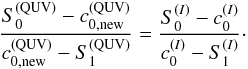 (B.1)In this way, we use
only local information, i.e. the shape of
SI(τ) and the endpoint
values of SQUV, to define the run of
SQUV(τ).
(B.1)In this way, we use
only local information, i.e. the shape of
SI(τ) and the endpoint
values of SQUV, to define the run of
SQUV(τ).
We note that in the DELO method of Rees et al.
(1989), the integration of the source functions is only part of the solution.
The determination of the full Stokes vector intensities requires the solution of a
system of linear equations. Even with our integration method, in very rare cases, the
solution of the equation system produces unphysical results with one or more Stokes
components becoming larger than Stokes I. Consequently, we changed the
RH code in such a way, that the polarized Stokes component fulfills the condition
 (B.2)
(B.2)
after each formal solution. In all of these cases in which the relation was not
fulfilled, the polarized components were reduced by a single factor f
(i.e. Qnew = fQ,
Unew = fU,
Vnew = fV) such that the equality in the
equation above held, i.e.  (B.3)
(B.3)
© ESO, 2012
Current usage metrics show cumulative count of Article Views (full-text article views including HTML views, PDF and ePub downloads, according to the available data) and Abstracts Views on Vision4Press platform.
Data correspond to usage on the plateform after 2015. The current usage metrics is available 48-96 hours after online publication and is updated daily on week days.
Initial download of the metrics may take a while.