© ESO 2020

1. Introduction

The constituent parts of the Λ cold dark matter (ΛCDM) model, and its extensions, are not all fully understood. In the current framework, there is no definitive explanation for the physical natures of dark matter and dark energy. Today, there are a variety of techniques available to better constrain our knowledge of the ΛCDM cosmological parameters. Cosmic shear, which is the distortion in the observed shapes of distant galaxies due to weak gravitational lensing by the large-scale structure of the Universe (LSS), is one such cosmological probe. By measuring this distortion over large samples of galaxies, the LSS can be explored. Given that the LSS depends on density fluctuations and the geometry of the Universe, this measurement allows for the constraining of cosmological parameters. In particular, it is a powerful tool to study dark energy (Albrecht et al. 2006). A three-dimensional, redshift-dependent, picture can be obtained using a technique known as tomography. In this technique, the observed galaxies are divided into different tomographic bins; each covering a different redshift range.

Since its debut at the turn of the millennium (Bacon et al. 2000; Kaiser et al. 2000; Van Waerbeke et al. 2000; Wittman et al. 2000; Rhodes et al. 2000), studies of cosmic shear have evolved to the point where multiple independent surveys have carried out precision cosmology (Dark Energy Survey Collaboration 2005; Heymans et al. 2012; Hildebrandt et al. 2017). Now, with the impending arrival of Stage IV (Albrecht et al. 2006) dark energy experiments, such as Euclid¹ (Laureijs et al. 2011), WFIRST² (Akeson et al. 2019), and LSST³ (LSST Science Collaboration et al. 2009), we are poised for a leap in precision. For example, even a pessimistic analysis of Euclid weak lensing data is projected to increase precision by a factor of ∼25 over current surveys (Sellentin & Starck 2019).

To ensure that the accuracy of the analysis keeps up with the increasing precision of the measurements, the impact of previously neglected physical effects must be evaluated. In cosmic shear a wide range of scales are probed, so the non-linear matter power spectrum must be precisely modelled. This can be accomplished through model fitting to N-body simulations (Smith et al. 2003; Takahashi et al. 2012). A robust understanding of how baryonic physics affects the matter power spectrum is also necessary (Rudd et al. 2008; Semboloni et al. 2013). Furthermore, spurious signals arising from intrinsic alignments (IAs; Joachimi et al. 2015; Kirk et al. 2015; Kiessling et al. 2015) in observed galaxy shapes need to be taken into account.

Additionally, assumptions in the theoretical formalism must also be relaxed. The effects of several such extensions on a Euclid-like experiment have been investigated. These include: the impacts of relaxing the Limber, Hankel transform and flat-sky approximations (Kitching et al. 2017), of using unequal-time correlators (Kitching & Heavens 2017), and of making the spatially-flat Universe approximation (Taylor et al. 2018).

The formalism to correct for the effect of measuring reduced shear, rather than shear itself, is known (Shapiro 2009; Krause & Hirata 2010). However, its impact on impending surveys has not yet been quantified. The correction to the two-point cosmic shear statistic for magnification bias is also known. While the impact of this on Stage IV experiments has been quantified in Liu et al. (2014), the approach taken here risks underestimating the bias for surveys covering the redshift range of Euclid. Rather than assuming that the magnification bias at the survey’s mean redshift is representative of the bias at all covered redshifts, a tomographic approach is required. Magnification bias also affects measurements of galaxy clustering; which is the other of Euclid’s major probes. Thiele et al. (2020), Lorenz et al. (2018), Duncan et al. (2014) study the impact of magnification on the clustering sample, and as such complement this work in forming a holistic picture of the effect on Euclid.

Conveniently, the magnification bias correction takes a mathematically similar form to that of reduced shear; meaning these corrections can be treated together (Schmidt et al. 2009). Within this work, we calculate the bias on the predicted cosmological parameters obtained from Euclid, when these two effects are neglected. We further extend the existing correction formalism to include the impact of IAs, and recompute the bias for this case.

In Sect. 2, we establish the theoretical formalism. We begin by summarising the standard, first-order, cosmic shear power spectrum calculation. We then review the basic reduced shear correction formalism of Shapiro (2009). Following this, the correction for magnification bias is explained. Next, the theory used to account for the IAs is examined. We then combine the discussed schemes, in order to create a description of an IA-enhanced lensing bias correction to the cosmic shear power spectrum. We also explain how we quantify the uncertainties and biases induced in the measured cosmological parameters.

In Sect. 3, we describe how we calculated the impact of the aforementioned corrections for Euclid. Our modelling assumptions and choice of fiducial cosmology are stated, and computational specifics are given.

Finally, in Sect. 4, our results are presented, and their implications for Euclid are discussed. The biases and change in confidence contours of cosmological parameters, resulting from the basic reduced shear and magnification bias corrections, are presented. We also present the biases from the IA-enhanced lensing bias correction.

2. Theoretical formalism

Here, we first review the standard cosmic shear calculation. We then explain the corrections required to account for the reduced shear approximation, and for magnification bias. We further consider the effects of IAs, and construct an IA-enhanced lensing bias correction. The formalism for accounting for the shot noise is then stated. Our chosen framework for predicting uncertainties and biases is also detailed.

2.1. The standard cosmic shear calculation

When a distant galaxy is weakly lensed, the change in its observed ellipticity is proportional to the reduced shear, g:

$$\begin{array}{c}\hfill g^{\alpha }(\mathit{\theta })=\frac{{\gamma }^{\alpha }(\mathit{\theta })}{1-\kappa (\mathit{\theta })},\end{array}$$(1)

where θ is the galaxy’s position on the sky, γ is the shear, which is an anisotropic stretching that turns circular distributions of light elliptical, and κ is the convergence, which is an isotropic change in the size of the image. The superscript, α, encodes the fact that the spin-2 shear has two components. Since |γ|, |κ| ≪ 1 for individual galaxies in weak lensing, Eq. (1) is typically approximated to first-order as g^α(θ) ≈ γ^α(θ). This is known as the reduced shear approximation.

The convergence of a source being weakly lensed by the LSS, in a tomographic redshift bin i, is given by:

$$\begin{array}{c}\hfill {\kappa }_i(\mathit{\theta })={\displaystyle {\int }_0^{{\chi }_{\lim }}}\mathrm{d}\chi \delta [d_{\mathrm{A}}(\chi )\mathit{\theta },\chi ]W_i(\chi ).\end{array}$$(2)

It is the projection of the density contrast of the Universe, δ, over the comoving distance, χ, along the line-of-sight, to the limiting comoving distance of the observed sample of sources, χ_lim. The function d_A(χ) accounts for the curvature of the Universe, K, depending on whether it is flat, open, or closed:

$$\begin{array}{c}\hfill d_{\mathrm{A}}(\chi )=\{\begin{array}{cc}{|K|}^{-1/2}{sin(|K|}^{-1/2}\chi )\hfill & K>0(\mathrm{Closed})\hfill \\ \chi \hfill & K=0(\mathrm{Flat})\hfill \\ {|K|}^{-1/2}{sinh(|K|}^{-1/2}\chi )\hfill & K<0(\mathrm{Open}),\hfill \end{array}\end{array}$$(3)

and W_i(χ) is the lensing kernel for sources in bin i, with the definition

$$\begin{array}{c}\hfill W_i(\chi )=\frac{3}{2}{\mathrm{\Omega }}_{\mathrm{m}}\frac{H_0^2}{c^2}\frac{d_{\mathrm{A}}(\chi )}{a(\chi )}{\displaystyle {\int }_{\chi }^{{\chi }_{\lim }}}\mathrm{d}{\chi }^{\prime }{n}_i({\chi }^{\prime })\frac{d_{\mathrm{A}}({\chi }^{\prime }-\chi )}{d_{\mathrm{A}}({\chi }^{\prime })}·\end{array}$$(4)

Here, Ω_m is the dimensionless present-day matter density parameter of the Universe, H₀ is the Hubble constant, c is the speed of light in a vacuum, a(χ) is the scale factor of the Universe, and n_i(χ) is the probability distribution of galaxies within bin i.

Meanwhile, the two shear components, for a bin i, when caused by a lensing mass distribution, can be related to the convergence in a straightforward manner in frequency space:

$$\begin{array}{c}\hfill {\stackrel{\sim }{\gamma }}_i^{\alpha }(\mathit{\ell })=\frac{1}{\ell (\ell +1)}\sqrt{\frac{(\ell +2)!}{(\ell -2)!}}{T}^{\alpha }(\mathit{\ell }){\stackrel{\sim }{\kappa }}_i(\mathit{\ell }),\end{array}$$(5)

where ℓ is the spherical harmonic conjugate of θ. Here, the small-angle limit is used. However, we do not apply the “prefactor unity” approximation (Kitching et al. 2017), in which the factor of $1/\ell (\ell +1)\sqrt{(\ell +2)!/(\ell -2)!}$ is taken to be one, despite the fact that the impact of making the approximation is negligible for a Euclid-like survey (Kilbinger et al. 2017). This is done to allow consistent comparison with the spherical-sky reduced shear and magnification bias corrections. The trigonometric weighting functions, T^α(ℓ), of the two shear components are defined as:

$$\begin{array}{cc}& T^1(\mathit{\ell })=cos(2{\varphi }_{\ell }),\hfill \end{array}$$(6)

$$\begin{array}{cc}& T^2(\mathit{\ell })=sin(2{\varphi }_{\ell }),\hfill \end{array}$$(7)

with ϕ_l being the angular component of vector ℓ which has magnitude ℓ. Then, for an arbitrary shear field (e.g. one estimated from data), the two shear components can be linearly combined to be represented as a curl-free E-mode, and a divergence-free B-mode:

$$\begin{array}{cc}& {\stackrel{\sim }{E}}_i(\mathit{\ell })={\displaystyle \sum _{\alpha }}{T}^{\alpha }{\stackrel{\sim }{\gamma }}_i^{\alpha }(\mathit{\ell }),\hfill \end{array}$$(8)

$$\begin{array}{cc}& {\stackrel{\sim }{B}}_i(\mathit{\ell })={\displaystyle \sum _{\alpha }\sum _{\beta }}{\epsilon }^{\alpha \beta }{T}^{\alpha }(\mathit{\ell }){\stackrel{\sim }{\gamma }}_i^{\beta }(\mathit{\ell }),\hfill \end{array}$$(9)

where ε^αβ is the two-dimensional Levi–Civita symbol, so that ε¹² = −ε²¹ = 1 and ε¹¹ = ε²² = 0. The B-mode vanishes in the absence of any higher-order systematic effects. Therefore, we can then define the E-mode angular auto-correlation and cross-correlation spectra, $C_{\ell ;ij}^{\gamma \gamma }$, as:

$$\begin{array}{c}\hfill ⟨{\stackrel{\sim }{E}}_i(\mathit{\ell }){\stackrel{\sim }{E}}_j({\mathit{\ell }}^{\prime })⟩={(2\pi )}^2{\delta }_{\mathrm{D}}^2(\mathit{\ell }+{\mathit{\ell }}^{\prime })C_{\ell ;ij}^{\gamma \gamma },\end{array}$$(10)

where ${\delta }_{\text{D}}^2$ is the two-dimensional Dirac delta function. From here, an expression is derived for $C_{\ell ;ij}^{\gamma \gamma }$:

$$\begin{array}{c}\hfill C_{\ell ;ij}^{\gamma \gamma }=\frac{(\ell +2)!}{(\ell -2)!}\frac{1}{{(\ell +1/2)}^4}{\displaystyle {\int }_0^{{\chi }_{\lim }}}\mathrm{d}\chi \frac{W_i(\chi )W_j(\chi )}{d_{\mathrm{A}}^2(\chi )}{P}_{\delta \delta }(k,\chi ),\end{array}$$(11)

where P_δδ(k, χ) is the three-dimensional matter power spectrum. Obtaining Eq. (11) relies on making the Limber approximation, that is, assuming that only ℓ-modes in the plane of the sky contribute to the lensing signal. Under the Limber approximation, k = (ℓ+1/2)/d_A(χ). In this equation, the factors of (ℓ+2)!/(ℓ−2)! and 1/(ℓ+1/2)⁴ come once again from the fact that the prefactor unity approximation is not used. For a comprehensive review, see Kilbinger (2015).

2.2. The reduced shear correction

We account for the effects of the reduced shear approximation by means of a second-order correction to Eq. (11) (Shapiro 2009; Krause & Hirata 2010; Dodelson et al. 2006). This can be done by taking the Taylor expansion of Eq. (1) around κ = 0, and keeping terms up to second-order:

$$\begin{array}{c}\hfill g^{\alpha }(\mathit{\theta })={\gamma }^{\alpha }(\mathit{\theta })+({\gamma }^{\alpha }\kappa )(\mathit{\theta })+\mathcal{O}({\kappa }^3).\end{array}$$(12)

By substituting this expanded form of g^α for γ^α in Eq. (8) and then recomputing the E-mode ensemble average, we obtain the original result of Eq. (10), plus a correction:

$$\begin{array}{cc}& \delta ⟨{\stackrel{\sim }{E}}_i(\mathit{\ell }){\stackrel{\sim }{E}}_j({\mathit{\ell }}^{\prime })⟩={(2\pi )}^2{\delta }_{\mathrm{D}}^2(\mathit{\ell }+{\mathit{\ell }}^{\prime })\delta C_{\ell ;ij}^{\mathrm{RS}}\hfill \\ \hfill & ={\displaystyle \sum _{\alpha }}{\displaystyle \sum _{\beta }}{T}^{\alpha }(\mathit{\ell })T^{\beta }({\mathit{\ell }}^{\prime })⟨{\stackrel{\sim }{({\gamma }^{\alpha }\kappa )}}_i(\mathit{\ell }){\stackrel{\sim }{\gamma }}_j^{\beta }({\mathit{\ell }}^{\prime })⟩\hfill \\ \hfill & +T^{\alpha }({\mathit{\ell }}^{\prime })T^{\beta }(\mathit{\ell })⟨{\stackrel{\sim }{({\gamma }^{\alpha }\kappa )}}_j({\mathit{\ell }}^{\prime }){\stackrel{\sim }{\gamma }}_i^{\beta }(\mathit{\ell })⟩,\hfill \end{array}$$(13)

where $\delta C_{\ell ;ij}^{\mathrm{RS}}$ are the resulting corrections to the angular auto and cross-correlation spectra. Applying the Limber approximation once more, we obtain an expression for these:

$$\begin{array}{cc}& \delta C_{\ell ;ij}^{\mathrm{RS}}=\ell (\ell +1)\frac{(\ell +2)!}{(\ell -2)!}\frac{1}{{(\ell +1/2)}^6}{\displaystyle {\int }_0^{\infty }}\frac{{\mathrm{d}}^2{\mathit{\ell }}^{\prime }}{{(2\pi )}^2}cos(2{\varphi }_{\ell }^{\prime }-2{\varphi }_{\ell })\hfill \\ \hfill & \times B_{\mathit{ij}}^{\kappa \kappa \kappa }(\mathit{\ell },{\mathit{\ell }}^{\prime },-\mathit{\ell }-{\mathit{\ell }}^{\prime }).\hfill \end{array}$$(14)

The factors of ℓ(ℓ + 1)(ℓ+2)!/(ℓ−2)! and 1/(ℓ+1/2)⁶ arise from foregoing the three-point equivalent of the prefactor unity approximation. As in the case of Eq. (5), the product of these factors can be well approximated by one. However, we do not make this approximation for the sake of completeness, and as the additional factors do not add any significant computational expense. Here, $B_{\mathit{ij}}^{\kappa \kappa \kappa }$ is the two-redshift convergence bispectrum, which takes the following form:

$$\begin{array}{cc}& B_{\mathit{ij}}^{\kappa \kappa \kappa }({\mathit{\ell }}_1,{\mathit{\ell }}_2,{\mathit{\ell }}_3)=B_{\mathit{iij}}^{\kappa \kappa \kappa }({\mathit{\ell }}_1,{\mathit{\ell }}_2,{\mathit{\ell }}_3)+B_{\mathit{ijj}}^{\kappa \kappa \kappa }({\mathit{\ell }}_1,{\mathit{\ell }}_2,{\mathit{\ell }}_3)\hfill \\ \hfill & ={\displaystyle {\int }_0^{{\chi }_{\lim }}}\frac{\mathrm{d}\chi }{d_{\mathrm{A}}^4(\chi )}{W}_i(\chi )W_j(\chi )[W_i(\chi )+W_j(\chi )]\hfill \\ \hfill & \times B_{\delta \delta \delta }({\mathit{k}}_1,{\mathit{k}}_2,{\mathit{k}}_3,\chi ),\hfill \end{array}$$(15)

where $B_{\mathit{iij}}^{\kappa \kappa \kappa }$ and $B_{\mathit{ijj}}^{\kappa \kappa \kappa }$ are the three-redshift bispectra, k_x is the magnitude and ϕ_ℓ; x is the angular component of k_x (for x = 1, 2, 3). Under the Limber approximation, k_x = (ℓ_x + 1/2)/d_A(χ). Here, we also approximate our photometric redshift bins to be infinitesimally narrow. In reality, because these bins would have a finite width, the product of lensing kernels in Eq. (15) would be replaced by a single integral over the products of the contents of the integral in Eq. (4). Accordingly, the values of the bispectrum would be slightly higher. However, given that Euclid will have high quality photometric redshift measurement, we expect this difference to be negligible. Consequently, in our calculations we proceeded with the narrow-bin approximation, which allowed us to use the same lensing kernels as used in the power spectrum calculation.

Analogous to the first-order power spectra being projections of the three-dimensional matter power spectrum, the two-dimensional convergence bispectra are a projection of the three-dimensional matter bispectrum, B_δδδ(k₁, k₂, k₃, χ). The analytic form of the matter bispectrum is not well known. Instead, a semi-analytic approach starting with second-order perturbation theory (Fry 1984), and then fitting its result to N-body simulations, is employed. We used the fitting formula of Scoccimarro & Couchman (2001). Accordingly, the matter bispectrum can be written:

$$\begin{array}{cc}& B_{\delta \delta \delta }({\mathit{k}}_1,{\mathit{k}}_2,{\mathit{k}}_3,\chi )=2F_2^{\mathrm{eff}}({\mathit{k}}_1,{\mathit{k}}_2)P_{\delta \delta }(k_1,\chi )P_{\delta \delta }(k_2,\chi )+\mathrm{cyc}.,\hfill \end{array}$$(16)

where $F_2^{\text{eff}}$ encapsulates the simulation fitting aspect, and is defined as:

$$\begin{array}{cc}& F_2^{\mathrm{eff}}({\mathit{k}}_1,{\mathit{k}}_2)=\frac{5}{7}a(n_{\mathrm{s}},k_1)a(n_{\mathrm{s}},k_2)\hfill \\ \hfill & +\frac{1}{2}\frac{{\mathit{k}}_1·{\mathit{k}}_2}{k_1{k}_2}(\frac{k_1}{k_2}+\frac{k_2}{k_1})b(n_{\mathrm{s}},k_1)b(n_{\mathrm{s}},k_2)\hfill \\ \hfill & +\frac{2}{7}(\frac{{\mathit{k}}_1·{\mathit{k}}_2}{k_1{k}_2}{)}^{2}c(n_{\mathrm{s}},k_1)c(n_{\mathrm{s}},k_2),\hfill \end{array}$$(17)

where n_s is the scalar spectral index, which indicates the deviation of the primordial matter power spectrum from scale invariance (n_s = 1), and the functions a, b, and c are fitting functions, defined in Scoccimarro & Couchman (2001). There are no additional correction terms of form $\stackrel{\sim }{\mathrm{E}}\stackrel{\sim }{\mathrm{B}}$ or $\stackrel{\sim }{\mathrm{B}}\stackrel{\sim }{\mathrm{B}}$, and it has been shown that higher-order terms are sub-dominant (Krause & Hirata 2010), so further terms in Eq. (12) can be neglected for now.

2.3. The magnification bias correction

The observed overdensity of galaxies on the sky is affected by gravitational lensing in two competing ways (Turner et al. 1984). Firstly, individual galaxies can be magnified (or demagnified), which results in their flux being increased (or decreased). At the flux limit of a survey, this can cause fainter sources (which in the absence of lensing would be excluded) to be included in the observed sample. Conversely, the density of galaxies in the patch of sky around this source appears reduced (or increased) due to the patch of sky being magnified (or demagnified) similarly to the source. Accordingly, the net effect of these depends on the slope of the intrinsic, unlensed, galaxy luminosity function, at the survey’s flux limit. This net effect is known as magnification bias. Additionally, galaxies can also be pulled into a sample because their effective radius is increased as a consequence of magnification, such that they pass a resolution factor cut. In this work, we do not consider this effect as it is more important for ground-based surveys than space-based ones such as Euclid.

In the case of weak lensing, where |κ|≪1, and assuming that fluctuations in the intrinsic galaxy overdensity are small on the scales of interest, the observed galaxy overdensity in tomographic bin i is (Hui et al. 2007; Turner et al. 1984):

$$\begin{array}{c}\hfill {\delta }_{\mathrm{obs};i}^{\mathrm{g}}(\mathit{\theta })={\delta }_i^{\mathrm{g}}(\mathit{\theta })+(5s_i-2){\kappa }_i(\mathit{\theta }),\end{array}$$(18)

where ${\delta }_i^g(\mathit{\theta })$ is the intrinsic, unlensed, galaxy overdensity in bin i, and s_i is the slope of the cumulative galaxy number counts brighter than the survey’s limiting magnitude, m_lim, in redshift bin i. This slope is defined as:

$$\begin{array}{c}\hfill s_i=\frac{\partial {\log }_{10}\mathfrak{n}(\overline{z_i},m)}{\partial m}{|}_{m_{\lim }},\end{array}$$(19)

where $\mathfrak{n}({\overline{z}}_i,m)$ is the true distribution of galaxies, evaluated at the central redshift of bin i, $\overline{z_i}$. It is important to note that, in practice, this slope is determined from observations, and accordingly depends on the wavelength band within which the galaxy is observed in addition to its redshift.

Operationally, magnification bias causes the true shear, ${\gamma }_i^{\alpha }$, to be replaced, within the estimator used to determine the power spectrum from data, by an “observed” shear:

$$\begin{array}{c}\hfill {\gamma }_{\mathrm{obs};i}^{\alpha }{\stackrel{\gamma }{\to }}_i^{\alpha }+{\gamma }_i^{\alpha }{\delta }_{\mathrm{obs};i}^g={\gamma }_i^{\alpha }+{\gamma }_i^{\alpha }{\delta }_i^g+(5s_i-2){\gamma }_i^{\alpha }{\kappa }_i.\end{array}$$(20)

Now, we can evaluate the impact of magnification bias on the two-point statistic by substituting ${\stackrel{\sim }{\gamma }}_{\mathrm{obs};i}^{\alpha }$ for ${\stackrel{\sim }{\gamma }}_i^{\alpha }$ in Eq. (8), and recomputing. As source-lens clustering terms of the form ${\gamma }_i^{\alpha }{\delta }_i^g$ are negligible (Schmidt et al. 2009), we recover the standard result of Eq. (10), with an additional correction term:

$$\begin{array}{cc}& \delta ⟨{\stackrel{\sim }{E}}_i(\mathit{\ell }){\stackrel{\sim }{E}}_j({\mathit{\ell }}^{\prime })⟩={\displaystyle \sum _{\alpha }}{\displaystyle \sum _{\beta }}{T}^{\alpha }(\mathit{\ell })T^{\beta }({\mathit{\ell }}^{\prime })(5s_i-2)⟨{\stackrel{\sim }{({\gamma }^{\alpha }\kappa )}}_i(\mathit{\ell }){\stackrel{\sim }{\gamma }}_j^{\beta }({\mathit{\ell }}^{\prime })⟩\hfill \\ \hfill & +T^{\alpha }({\mathit{\ell }}^{\prime })T^{\beta }(\mathit{\ell })(5s_j-2)⟨{\stackrel{\sim }{({\gamma }^{\alpha }\kappa )}}_j({\mathit{\ell }}^{\prime }){\stackrel{\sim }{\gamma }}_i^{\beta }(\mathit{\ell })⟩.\hfill \end{array}$$(21)

Analogously to the reduced shear case, we then obtain corrections to the auto and cross-correlation angular spectra of the form:

$$\begin{array}{cc}& \delta C_{\ell ;ij}^{\mathrm{MB}}=\ell (\ell +1)\frac{(\ell +2)!}{(\ell -2)!}\frac{1}{{(\ell +1/2)}^6}{\displaystyle {\int }_0^{\infty }}\frac{{\mathrm{d}}^2{\mathit{\ell }}^{\prime }}{{(2\pi )}^2}cos(2{\varphi }_{\ell }^{\prime }-2{\varphi }_{\ell })\hfill \\ \hfill & \times [(5s_i-2)B_{\mathit{iij}}^{\kappa \kappa \kappa }(\mathit{\ell },{\mathit{\ell }}^{\prime },-\mathit{\ell }-{\mathit{\ell }}^{\prime })\hfill \\ \hfill & +(5s_j-2)B_{\mathit{ijj}}^{\kappa \kappa \kappa }(\mathit{\ell },{\mathit{\ell }}^{\prime },-\mathit{\ell }-{\mathit{\ell }}^{\prime })].\hfill \end{array}$$(22)

We note that the mathematical form of Eq. (22) is simply Eq. (14) with factors of (5s_i − 2) and (5s_j − 2) applied to the corresponding bispectra. These additional prefactors are due to the magnification bias contribution from each bin depending on the slope of the luminosity function in that bin. Accordingly, we are able to compute both of these effects for the computational cost of one.

2.4. Intrinsic alignments

When galaxies form near each other, they do so in a similar tidal field. Such tidal process occurring during galaxy formation, together with other processes such as spin correlations, can induce a preferred, intrinsically correlated, alignment of galaxy shapes (Joachimi et al. 2015; Kirk et al. 2015; Kiessling et al. 2015). To first-order, this can be thought of as an additional contribution to the observed ellipticity of a galaxy, ϵ:

$$\begin{array}{c}\hfill ϵ=\gamma +{\gamma }^{\mathrm{I}}+{ϵ}^s,\end{array}$$(23)

where γ = γ¹ + iγ² is the gravitational lensing shear, γ^I is the contribution to the observed shape resulting from IAs, and ϵ^s is the source ellipticity that the galaxy would have in the absence of the process causing the IA.

Using Eq. (23), we find that the theoretical two-point statistic (e.g. the two-point correlation function, or the power spectrum) consists of three types of terms: ⟨γγ⟩,⟨γ^Iγ⟩, and ⟨γ^Iγ^I⟩. The first of these terms leads to the standard lensing power spectra of Eq. (11), while the other two terms lead to additional contributions to the observed power spectra, $C_{\ell ;ij}^{ϵϵ}$, so that:

$$\begin{array}{c}\hfill C_{\ell ;ij}^{ϵϵ}=C_{\ell ;ij}^{\gamma \gamma }+C_{\ell ;ij}^{\mathrm{I}\gamma }+C_{\ell ;ij}^{\mathrm{II}}+N_{\ell ;ij}^{ϵ},\end{array}$$(24)

where $C_{\ell ;ij}^{\mathrm{I}\gamma }$ represents the correlation between the background shear and the foreground IA, $C_{\ell ;ij}^{\mathrm{II}}$ are the auto-correlation spectra of the IAs, and $N_{\mathcal{l};ij}^{ϵ}$ is a shot noise term. The additional spectra can be described in a similar manner to the shear power spectra, by way of the non-linear alignment (NLA) model (Bridle & King 2007):

$$\begin{array}{cc}& C_{\ell ;ij}^{\mathrm{I}\gamma }=\frac{(\ell +2)!}{(\ell -2)!}\frac{1}{{(\ell +1/2)}^4}{\displaystyle {\int }_0^{{\chi }_{\lim }}}\frac{\mathrm{d}\chi }{d_{\mathrm{A}}^2(\chi )}[W_i(\chi )n_j(\chi )\hfill \\ \hfill & +n_i(\chi )W_j(\chi )]P_{\delta \mathrm{I}}(k,\chi ),\hfill \end{array}$$(25)

$$\begin{array}{cc}& C_{\ell ;ij}^{\mathrm{II}}=\frac{(\ell +2)!}{(\ell -2)!}\frac{1}{{(\ell +1/2)}^4}{\displaystyle {\int }_0^{{\chi }_{\lim }}}\frac{\mathrm{d}\chi }{d_{\mathrm{A}}^2(\chi )}{n}_i(\chi )n_j(\chi )P_{\mathrm{II}}(k,\chi ),\hfill \end{array}$$(26)

where the intrinsic alignment power spectra, P_δI(k, χ) and P_II(k, χ), are expressed as functions of the matter power spectra:

$$\begin{array}{cc}\hfill P_{\delta \mathrm{I}}(k,\chi )& =\frac{-{\mathcal{A}}_{\mathrm{IA}}{\mathcal{C}}_{\mathrm{IA}}{\mathrm{\Omega }}_{\mathrm{m}}}{D(\chi )}{P}_{\delta \delta }(k,\chi ),\hfill \end{array}$$(27)

$$\begin{array}{cc}\hfill P_{\mathrm{II}}(k,\chi )& =(\frac{-{\mathcal{A}}_{\mathrm{IA}}{\mathcal{C}}_{\mathrm{IA}}{\mathrm{\Omega }}_{\mathrm{m}}}{D(\chi )}{)}^2{P}_{\delta \delta }(k,\chi ),\hfill \end{array}$$(28)

in which 𝒜_IA and 𝒞_IA are free model parameters to be determined by fitting to data or simulations, and D(χ) is the growth factor of density perturbations in the Universe, as a function of comoving distance.

2.5. IA-enhanced lensing bias

The reduced shear approximation is also used when considering the impact of IAs, and magnification bias plays a role here too. We account for these by substituting the appropriate second-order expansions of the shear, Eqs. (12) and (20), in place of γ within Eq. (23). Neglecting source-lens clustering, the ellipticity now becomes:

$$\begin{array}{c}\hfill ϵ\simeq \gamma +(1+5s-2)\gamma \kappa +{\gamma }^{\mathrm{I}}+{ϵ}^s.\end{array}$$(29)

Constructing a theoretical expression for the two-point statistic from this revised expression for the ellipticity now gives us six types of terms: ⟨γγ⟩,⟨γ^Iγ⟩,⟨γ^Iγ^I⟩,⟨(γκ)γ⟩,⟨(γκ)(γκ)⟩, and ⟨(γκ)γ^I⟩. The first three terms remain unchanged from the first-order case. The fourth term encompasses the basic reduced shear and magnification bias corrections, and results in the shear power spectrum corrections defined by Eqs. (14) and (22). The fifth of these terms can be neglected, as it is a fourth-order term. The final term creates an additional correction, $\delta C_{\ell ;ij}^{\mathrm{I}}$, to the observed spectra that takes a form analogous to the basic reduced shear and magnification bias corrections:

$$\begin{array}{cc}& \delta C_{\ell ;ij}^{\mathrm{I}}=\ell (\ell +1)\frac{(\ell +2)!}{(\ell -2)!}\frac{1}{{(\ell +1/2)}^6}{\displaystyle {\int }_0^{\infty }}\frac{{\mathrm{d}}^2{\mathit{\ell }}^{\prime }}{{(2\pi )}^2}cos(2{\varphi }_{\ell }^{\prime })\hfill \\ \hfill & \times [(1+5s_i-2)B_{\mathit{iij}}^{\kappa \kappa \mathrm{I}}(\mathit{\ell },{\mathit{\ell }}^{\prime },-\mathit{\ell }-{\mathit{\ell }}^{\prime })\hfill \\ \hfill & +(1+5s_j-2)B_{\mathit{jji}}^{\kappa \kappa \mathrm{I}}(\mathit{\ell },{\mathit{\ell }}^{\prime },-\mathit{\ell }-{\mathit{\ell }}^{\prime })],\hfill \end{array}$$(30)

where the convergence-IA bispectra, $B_{\mathit{iij}}^{\kappa \kappa \mathrm{I}}$ and $B_{\mathit{jji}}^{\kappa \kappa \mathrm{I}}$, are given by:

$$\begin{array}{cc}& B_{\mathit{iij}}^{\kappa \kappa \mathrm{I}}({\mathit{\ell }}_1,{\mathit{\ell }}_2,{\mathit{\ell }}_3)={\displaystyle {\int }_0^{{\chi }_{\lim }}}\frac{\mathrm{d}\chi }{d_{\mathrm{A}}^4(\chi )}{W}_i^2(\chi )n_j(\chi )B_{\delta \delta \mathrm{I}}({\mathit{k}}_1,{\mathit{k}}_2,{\mathit{k}}_3,\chi ),\hfill \end{array}$$(31)

$$\begin{array}{cc}& B_{\mathit{jji}}^{\kappa \kappa \mathrm{I}}({\mathit{\ell }}_1,{\mathit{\ell }}_2,{\mathit{\ell }}_3)={\displaystyle {\int }_0^{{\chi }_{\lim }}}\frac{\mathrm{d}\chi }{d_{\mathrm{A}}^4(\chi )}{W}_j^2(\chi )n_i(\chi )B_{\delta \delta \mathrm{I}}({\mathit{k}}_1,{\mathit{k}}_2,{\mathit{k}}_3,\chi ).\hfill \end{array}$$(32)

The density perturbation-IA bispectrum, B_δδI(k₁, k₂, k₃, χ), can be calculated in a similar way to the matter density perturbation bispectrum, using perturbation theory and the Scoccimarro & Couchman (2001) fitting formula. Accordingly:

$$\begin{array}{cc}& B_{\delta \delta \mathrm{I}}({\mathit{k}}_1,{\mathit{k}}_2,{\mathit{k}}_3,\chi )=2F_2^{\mathrm{eff}}({\mathit{k}}_1,{\mathit{k}}_2)P_{\mathrm{I}\delta }(k_1,\chi )P_{\delta \delta }(k_2,\chi )\hfill \\ \hfill & +2F_2^{\mathrm{eff}}({\mathit{k}}_2,{\mathit{k}}_3)P_{\delta \delta }(k_2,\chi )P_{\delta \mathrm{I}}(k_3,\chi )\hfill \\ \hfill & +2F_2^{\mathrm{eff}}({\mathit{k}}_1,{\mathit{k}}_3)P_{\delta \mathrm{I}}(k_1,\chi )P_{\delta \delta }(k_3,\chi ),\hfill \end{array}$$(33)

with P_Iδ(k₁, χ) = P_δI(k₁, χ). This equation is an ansatz for how IAs behave in the non-linear regime, analogous to the NLA model. The described approach, and in particular the fitting functions, remain valid because, in the NLA model, we can treat IAs as a field proportional, by some redshift-dependence weighting, to the matter density contrast. Since the fitting functions, $F_2^{\text{eff}}$, do not depend on the comoving distance, they remain unchanged. For the full derivation of this bispectrum term, and a generalisation for similar terms, see Appendix A.

2.6. Shot noise

The shot noise term in Eq. (24) arises from the uncorrelated part of the unlensed source ellipticities; represented by ϵ^s in Eq. (23). This is zero for cross-correlation spectra, because the ellipticities of galaxies at different comoving distances should be uncorrelated. However, it is non-zero for auto-correlation spectra. It is written as:

$$\begin{array}{c}\hfill N_{\ell ;ij}^{ϵ}=\frac{{\sigma }_{ϵ}^2}{{\overline{n}}_{\mathrm{g}}/N_{\mathrm{bin}}}{\delta }_{\mathit{ij}}^{\mathrm{K}},\end{array}$$(34)

where ${\sigma }_{ϵ}^2$ is the variance of the observed ellipticities in the galaxy sample, ${\overline{n}}_{\mathrm{g}}$ is the galaxy surface density of the survey, N_bin is the number of tomographic bins used, and ${\delta }_{\mathit{ij}}^{\mathrm{K}}$ is the Kronecker delta. Equation (34) assumes the bins are equi-populated.

2.7. Fisher and bias formalism

To estimate the uncertainty on cosmological parameters that will be obtained from Euclid, we used the Fisher matrix approach (Tegmark et al. 2015; Euclid Collaboration et al. 2019). In this formalism, the Fisher matrix is defined as the expectation of the Hessian of the likelihood:

$$\begin{array}{c}\hfill F_{\tau \zeta }=\langle \frac{-{\partial }^{2}lnL}{\partial {\theta }_{\tau }\partial {\theta }_{\zeta }}\rangle ,\end{array}$$(35)

where L is the likelihood of the parameters given the data, and τ and ζ refer to parameters of interest, θ_τ and θ_ζ. Assuming a Gaussian likelihood, the Fisher matrix can be rewritten in terms of only the covariance of the data, C, and the mean of the data vector, μ:

$$\begin{array}{c}\hfill F_{\tau \zeta }=\frac{1}{2}\mathrm{tr}[\frac{\partial \mathit{C}}{\partial {\theta }_{\tau }}{\mathit{C}}^{-1}\frac{\partial \mathit{C}}{\partial {\theta }_{\zeta }}{\mathit{C}}^{-1}]+{\displaystyle \sum _{\mathit{pq}}}\frac{\partial {\mu }_p}{\partial {\theta }_{\tau }}{({\mathit{C}}^{-1})}_{\mathit{pq}}\frac{\partial {\mu }_q}{\partial {\theta }_{\zeta }},\end{array}$$(36)

where the summations over p and q are summations over the variables in the data vector. In the case of cosmic shear, we can take our signal to be the mean of the power spectrum, so the first term in Eq. (36) vanishes.

In reality, the weak lensing likelihood is non-Gaussian (see e.g. Sellentin et al. 2018). However, recent investigations indicate that the assumption of a Gaussian likelihood is unlikely to lead to significant biases in the cosmological parameters inferred from a Stage IV weak lensing experiment (Lin et al. 2019; Taylor et al. 2019). Additionally, while this non-Gaussianity affects the shapes of the constraints on cosmological parameters, it does not affect the calculation of the reduced shear and magnification bias corrections, and accordingly does not significantly affect the corresponding relative biases. For these reasons, coupled with its simplicity, we proceed under the Gaussian likelihood assumption for this work.

Similarly, the covariance of the data itself is non-Gaussian. But, in contrast with the likelihood, we cannot assume a Gaussian covariance for cosmic shear (see e.g. Barreira et al. 2018; Takada & Hu 2013). The dominant contribution to the non-Gaussian part of the covariance is the super-sample covariance (SSC; Hu & Kravtsov 2003). This additional component arises from the fact that, in any galaxy survey, a limited fraction of the Universe is observed. Density fluctuations with wavelengths larger than the size of the survey can then cause the background density measured by the survey to no longer be representative of the true average density of the Universe. Additional non-Gaussian contributions, such as connected trispectrum terms, can be safely neglected for Euclid (Barreira et al. 2018).

For weak lensing, the covariance can then be expressed as the sum of the Gaussian, Cov_G, and SSC, Cov_SSC, parts:

$$\begin{array}{cc}& \mathrm{Cov}[C_{\ell ;ij}^{ϵϵ},C_{{\ell }^{\prime };mn}^{ϵϵ}]={\mathrm{Cov}}_{\mathrm{G}}[C_{\ell ;ij}^{ϵϵ},C_{{\ell }^{\prime };mn}^{ϵϵ}]\hfill \\ \hfill & +{\mathrm{Cov}}_{\mathrm{SSC}}[C_{\ell ;ij}^{ϵϵ},C_{{\ell }^{\prime };mn}^{ϵϵ}],\hfill \end{array}$$(37)

where (i, j) and (m, n) are redshift bin pairs. The Gaussian covariance is given by:

$$\begin{array}{cc}\hfill {\mathrm{Cov}}_{\mathrm{G}}[C_{\ell ;ij}^{ϵϵ},C_{{\ell }^{\prime };mn}^{ϵϵ}]& =\frac{C_{\ell ;im}^{ϵϵ}{C}_{{\ell }^{\prime };jn}^{ϵϵ}+C_{\ell ;in}^{ϵϵ}{C}_{{\ell }^{\prime };jm}^{ϵϵ}}{(2\ell +1)f_{\mathrm{sky}}\mathrm{\Delta }\ell }{\delta }_{\ell {\ell }^{\prime }}^{\mathrm{K}},\hfill \end{array}$$(38)

where δ^K is the Kronecker delta, Δℓ is the bandwidth of ℓ-modes sampled, and f_sky is the fraction of the sky surveyed. The contribution from SSC can be approximated as (Lacasa & Grain 2019):

$$\begin{array}{c}\hfill {\mathrm{Cov}}_{\mathrm{SSC}}[C_{\ell ;ij}^{ϵϵ},C_{{\ell }^{\prime };mn}^{ϵϵ}]\approx R_{\ell }{C}_{\ell ;ij}^{ϵϵ}{R}_{\ell }{C}_{{\ell }^{\prime };mn}^{ϵϵ}{S}_{\mathit{ijmn}},\end{array}$$(39)

where S_ijmn is the dimensionless volume-averaged covariance of the background matter density contrast, and R_ℓ is the effective relative response of the observed power spectrum.

The specific Fisher matrix used in this investigation can be expressed as:

$$\begin{array}{c}\hfill F_{\tau \zeta }^{\mathrm{G}}={\displaystyle \sum _{l^{\prime }={\ell }_{\min }}^{{\ell }_{\max }}\sum _{\ell ={\ell }_{\min }}^{{\ell }_{\max }}\sum _{ij,mn}}\frac{\partial C_{\ell ;ij}^{ϵϵ}}{\partial {\theta }_{\tau }}{\mathrm{Cov}}^{-1}[C_{\ell ;ij}^{ϵϵ},C_{l^{\prime }mn}^{ϵϵ}]\frac{\partial C_{l^{\prime }mn}^{ϵϵ}}{\partial {\theta }_{\zeta }},\end{array}$$(40)

where (ℓ_min, ℓ_max) are the minimum and maximum angular wavenumbers used, and the sum is over the ℓ-blocks.

From this, we can calculate the expected uncertainties on our parameters, σ_τ, using the relation:

$$\begin{array}{c}\hfill {\sigma }_{\tau }=\sqrt{{(F^{-1})}_{\tau \tau }}.\end{array}$$(41)

The Fisher matrix can also be used to determine the projected confidence region ellipses of pairs of cosmological parameters (Euclid Collaboration et al. 2019).

In the presence of a systematic effect in the signal, the Fisher matrix formalism can be adapted to measure how biased the inferred cosmological parameter values are if this effect is not taken into consideration (Taylor et al. 2007). This bias is calculated as follows:

$$\begin{array}{cc}\hfill b({\theta }_{\tau })& ={\displaystyle \sum _{\zeta }}{(F^{-1})}_{\tau \zeta }{B}_{\zeta },\hfill \end{array}$$(42)

with:

$$\begin{array}{cc}& B_{\zeta }={\displaystyle \sum _{l^{\prime }={\ell }_{\min }}^{{\ell }_{\max }}\sum _{\ell ={\ell }_{\min }}^{{\ell }_{\max }}\sum _{ij,mn}}\delta C_{\ell ;ij}{\mathrm{Cov}}^{-1}[C_{\ell ;ij}^{ϵϵ},C_{l^{\prime }mn}^{ϵϵ}]\frac{\partial C_{l^{\prime }mn}}{\partial \zeta },\hfill \end{array}$$(43)

where δC_ℓ; ij is the value of the systematic effect for bins (i, j), in our case reduced shear and magnification bias.

3. Methodology

In order to quantify the impact of the three corrections on Euclid, we adopted the forecasting specifications of Euclid Collaboration et al. (2019). Accordingly, we took there to be ten equi-populated tomographic bins, with bin edges: {0.001, 0.418, 0.560, 0.678, 0.789, 0.900, 1.019, 1.155, 1.324, 1.576, 2.50}. We primarily investigated the impact on the “optimistic” case for such a survey, in which ℓ-modes of up to 5000 are probed, because this is necessary for Euclid to reach its required figure of merit using cosmic shear (Euclid Collaboration et al. 2019). For the “pessimistic” case, see Appendix B. We considered the intrinsic variance of observed ellipticities to have two components, each with a value of 0.21, so that the intrinsic ellipticity root-mean-square value ${\sigma }_{ϵ}=\sqrt{2}\times 0.21\approx 0.3$. For Euclid, we took the surface density of galaxies to be ${\overline{n}}_{\mathrm{g}}=30$ arcmin⁻², and the fraction of sky covered to be f_sky = 0.36.

Furthermore, we considered the wCDM model case in our calculations. This extension of the ΛCDM model accounts for a time-varying dark energy equation of state. In this model, we have the following parameters: the present-day matter density parameter Ω_m, the present-day baryonic matter density parameter Ω_b, the Hubble parameter h = H₀/100 km s⁻¹ Mpc⁻¹, the spectral index n_s, the RMS value of density fluctuations on 8 h⁻¹ Mpc scales σ₈, the present-day dark energy density parameter Ω_DE, the present-day value of the dark energy equation of state w₀, and the high redshift value of the dark energy equation of state w_a. Additionally, we assumed neutrinos to have masses. We denote the sum of neutrino masses by ∑m_ν ≠ 0. This quantity was kept fixed, and we did not generate confidence contours for it, in concordance with Euclid Collaboration et al. (2019). The fiducial values chosen for these parameters are given in Table 1. These values were chosen to allow for a direct and consistent comparison of the two corrections with the forecasted precision of Euclid. The values provided in the forecasting specifications for the free parameters of the NLA model were also used in our work, in Eqs. (27) and (28). These are: 𝒜_IA = 1.72 and 𝒞_IA = 0.0134.

As in Euclid Collaboration et al. (2019), we chose to define the distributions of galaxies in our tomographic bins, for photometric redshift estimates, as:

$$\begin{array}{c}\hfill {\mathcal{N}}_i(z)=\frac{{\int }_{z_i^{-}}^{z_i^{+}}\mathrm{d}{z}_{\mathrm{p}}\mathfrak{n}(z)p_{\mathrm{ph}}(z_{\mathrm{p}}|z)}{{\int }_{z_{\min }}^{z_{\max }}\mathrm{d}z{\int }_{z_i^{-}}^{z_i^{+}}\mathrm{d}{z}_{\mathrm{p}}\mathfrak{n}(z)p_{\mathrm{ph}}(z_{\mathrm{p}}|z)},\end{array}$$(44)

where z_p is measured photometric redshift, $z_i^{-}$ and $z_i^{+}$ are edges of the ith redshift bin, and z_min and z_max define the range of redshifts covered by the survey. Then, n_i(χ) = 𝒩_i(z)dz/dχ. In Eq. (44), 𝔫(z) is the true distribution of galaxies with redshift, z; defined as in the Euclid Red Book (Laureijs et al. 2011):

$$\begin{array}{c}\hfill \mathfrak{n}(z)\propto (\frac{z}{z_0}{)}^2\exp [-(\frac{z}{z_0}{)}^{3/2}],\end{array}$$(45)

where $z_0=z_{\mathrm{m}}/\sqrt{2}$, with z_m = 0.9 as the median redshift of the survey. Meanwhile, the function p_ph(z_p|z) describes the probability that a galaxy at redshift z is measured to have a redshift z_p, and takes the parameterisation:

$$\begin{array}{cc}& p_{\mathrm{ph}}(z_{\mathrm{p}}|z)=\frac{1-f_{\mathrm{out}}}{\sqrt{2\pi }{\sigma }_{\mathrm{b}}(1+z)}\exp \{-\frac{1}{2}[\frac{z-c_{\mathrm{b}}{z}_{\mathrm{p}}-z_{\mathrm{b}}}{{\sigma }_{\mathrm{b}}(1+z)}{]}^2\}\hfill \\ \hfill & +\frac{f_{\mathrm{out}}}{\sqrt{2\pi }{\sigma }_{\mathrm{o}}(1+z)}\exp \{-\frac{1}{2}[\frac{z-c_{\mathrm{o}}{z}_{\mathrm{p}}-z_{\mathrm{o}}}{{\sigma }_{\mathrm{o}}(1+z)}{]}^2\}.\hfill \end{array}$$(46)

In this parameterisation, the first term describes the multiplicative and additive bias in redshift determination for the fraction of sources with a well measured redshift, whereas the second term accounts for the effect of a fraction of catastrophic outliers, f_out. The values of these parameters, chosen to match the selection of Euclid Collaboration et al. (2019), are stated in Table 2. By using this formalism, the impact of the photometric redshift uncertainties was also included in the derivatives, with respect to the cosmological parameters, of the shear power spectra.

The matter density power spectrum and growth factor used in our analyses were computed using the publicly available CLASS⁴ cosmology package (Blas et al. 2011). Within the framework of CLASS, we included non-linear corrections to the matter density power spectrum, using the Halofit model (Takahashi et al. 2012). Using these modelling specifics, we first calculated the basic reduced shear correction of Eq. (14), and the resulting biases in the wCDM parameters. In doing so, we computed the derivatives of our tomographic matrices, at each sampled ℓ-mode, using a simple finite-difference method. To calculate the dimensionless volume-averaged covariance of the background matter density contrast of Eq. (39), we used the publicly available PySSC⁵ code (Lacasa & Grain 2019) to compute the fullsky value, and divided by the Euclid value of f_sky. Additionally, we set R_ℓ ≈ 4 for weak lensing⁶.

Our Fisher matrices included the parameters Ω_m, Ω_b, h, n_s, σ₈, Ω_DE, w₀, w_a, and 𝒜_IA. We did not include any additional nuisance parameters. However, we do not expect this to affect the significance of the corrections, as Euclid Collaboration et al. (2019) find that the inclusion of various nuisance parameters typically alters the predicted relative uncertainties on cosmological parameters by less than 10%. No prior was added to our Fisher matrix analysis.

The correction for magnification bias, and the resulting biases in the cosmological parameters, were calculated in the same way. The slope of the luminosity function, as defined in Eq. (19), was calculated for each redshift bin using the approach described in Appendix C of Joachimi & Bridle (2010). We applied a finite-difference method to the fitting formula for galaxy number density as a function of limiting magnitude stated here, in order to calculate the slope of the luminosity function at the limiting magnitude of Euclid, 24.5 (Laureijs et al. 2011); or AB in the Euclid VIS band (Cropper et al. 2012). This technique produces slope values consistent with those generated from the Schechter function approach of Liu et al. (2014). The calculated slopes for each redshift bin are given in Table 3. However, we emphasise that while this method allows the investigation of the impact of magnification bias at this stage, when the correction is computed for the true Euclid data, updated galaxy number counts determined directly from Euclid observations should be used to ensure accuracy.

We then combined the two corrections, and calculated the resulting biases, as well as the resulting confidence contours for parameter combinations. Next, the additional IA-lensing bias interaction term from Eq. (30) was included, and the biases were recomputed.

To validate the perturbative formalism based on a fitting formula for the matter bispectrum, we also computed the reduced shear correction using a forward model approach assuming the lognormal field approximation (Hilbert et al. 2011; Mancini et al. 2018; Xavier et al. 2016). This approximation was recently used to generate a covariance matrix in the Dark Energy Survey Year 1 analysis (Troxel et al. 2018). Using the pipeline recently presented in Taylor et al. (2019) (which uses the public code CAMB (Lewis et al. 2000), Halofit (Takahashi et al. 2012), Cosmosis (Zuntz et al. 2015) and the python wrapper of HEALpix⁷ (Górski et al. 1999, 2005) – HEALpy) we computed the reduced shear correction by averaging over 100 forward realisations. We compared our semi-analytic approach to the forward modelled approach, for the auto-correlation spectrum of a single tomographic bin spanning the entire redshift range of 0–2.5. To ensure a consistent comparison was made with the forward model approach, the correction computed from the perturbative formalism in this case used the best-fitting photometric redshift galaxy distribution of the CFHTLenS catalogue (Van Waerbeke et al. 2013):

$$\begin{array}{c}\hfill \mathfrak{n}(z)=1.5\exp [-\frac{{(z-0.7)}^2}{0.1024}]+0.2\exp [-\frac{{(z-1.2)}^2}{0.2116}],\end{array}$$(47)

as this is used in Taylor et al. (2019). In this comparison, we did not consider magnification bias, or the IA-enhanced lensing bias case.

4. Results and discussion

In this section, we report the impact of the various effects studied on Euclid. We first present the individual and combined impacts of the reduced shear and magnification bias corrections. The impact of IA-enhanced lensing bias is also discussed. Finally, we present a forward modelled approach for computing the reduced shear correction.

4.1. The reduced shear correction

The relative magnitude of the basic reduced shear correction described by Eq. (14), to the observed shear auto-correlation spectra (excluding shot noise), at various redshifts, is shown in Fig. 1. The correction increases with ℓ, and becomes particularly pronounced at scales above ℓ ∼ 100. This is expected, as small-scale modes grow faster in high-density regions, where the convergence tends to be greater, so there is more power in these regions. We can also see, from Fig. 1, that the relative magnitude of the correction increases with redshift, as the reduced shear correction has an extra factor of the lensing kernel, W_i(χ), in comparison to the angular shear spectra. The lensing kernel increases with comoving distance and, accordingly, redshift. While only a selection of auto-correlation spectra are presented in Fig. 1 for illustration purposes, the remaining auto and cross-correlation spectra exhibit the same trends.

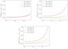Fig. 1. Reduced shear (top left), magnification bias (top right), and combined (bottom) corrections relative to the observed angular shear auto-correlation spectra (excluding shot noise), for four different redshift bins. For the basic reduced shear correction, the relative size of the correction increases alongside redshift, as the correction term has an additional factor of the lensing kernel compared to the power spectra. The correction plateaus at higher redshifts, because the lensed light encounters the most non-linearity and clustering at lower redshifts. It also increases with ℓ, as convergence tends to be higher on smaller physical scales. For the basic magnification bias correction, the relative size of the correction also increases with redshift. At lower redshifts, the term is subtractive, as the magnification of individual galaxies dominates, leading to an overestimation of the galaxy density. Whereas, at higher redshifts, the dilution of galaxy density dominates, leading to an underestimation of the power spectra if the correction is not made. For the combined effect of the two corrections, the magnification bias correction effectively cancels out the reduced shear correction at the lowest redshifts. Meanwhile, at intermediate redshifts, the magnification bias is small, but additive; slightly enhancing the reduced shear correction. However, at the highest redshifts, the magnification bias is particularly strong, and the combined correction is significantly greater than at lower redshifts. The corrections seen here are in the case of the wCDM cosmology of Table 1.

The uncertainties on the wCDM cosmological parameters that are predicted for Euclid, are stated in Table 4. Correspondingly, Table 5 shows the biases that are induced in the predicted cosmological parameters from neglecting the basic reduced shear correction.

Biases are typically considered acceptable when the biased and unbiased confidence regions have an overlap of at least 90%; corresponding to the magnitude of the bias being < 0.25σ (Massey et al. 2013). The majority of the biases are not significant, with Ω_m, Ω_b, h, n_s, and σ₈ remaining strongly consistent pre- and post-correction. However, Ω_DE, w₀, and w_a, all exhibit significant biases of 0.31σ, −0.32σ, and 0.39σ, respectively. Since one of the chief goals of upcoming weak lensing surveys is the inference of dark energy parameters, these biases, which can be readily dealt with, indicate that the reduced shear correction must be included when constraining cosmological parameters from the surveys. Also shown in Table 4 is the change in the uncertainty itself, when the reduced shear correction and its derivatives are included in the Fisher matrix used for prediction. In general, the change is negligible, because the reduced shear correction and its derivatives are relatively small in comparison to the shear spectra and derivatives. In the absence of any corrections, there are near-exact degeneracies which result in large uncertainties when the Fisher matrix is inverted. However, because we are dealing with near-zero eigenvalues in the Fisher matrix, even subtle changes to the models that encode information can significantly change the resulting parameter constraints.

Since the reduced shear correction depends on the observed density of baryonic matter, including it slightly improves the constraint on Ω_b. Also, the predicted uncertainties on h are also reduced, as the correction term has an additional factor of the lensing kernel relative to the angular power spectrum; increasing sensitivity to h by a power of two. The fitting formulae used to describe the matter bispectrum, as part of the correction term, also have a non-trivial dependence on n_s. This means that the sensitivity to n_s is also increased, when the correction is made.

On the other hand, the uncertainty on Ω_DE worsens upon correcting for the reduced shear approximation. This stems from the fact that the derivative of the correction term with respect to Ω_DE is negative, as a higher dark energy density results in a Universe that has experienced a greater rate of expansion, and accordingly is more sparsely populated with matter. Then, convergence in general is lower, and the magnitude of the correction drops as the approximation is more accurate. Therefore, the magnitude of the reduced shear correction and the strength of the Ω_DE signal are inversely correlated. This means that in the case where the reduced shear correction is made, Ω_DE is less well constrained than in the case where there is no correction. Conversely, increasing w₀ and w_a decreases the rate of expansion of the Universe, and so sensitivity to w₀ and w_a increases in the case when the correction is made.

4.2. The magnification bias correction

Figure 1 shows the magnitude of the basic magnification bias correction, relative to the shear auto-correlation spectra (again excluding shot noise). In this case, the relative magnitude of the correction again increases with redshift. However, in the two lowest redshift bins shown, the correction is subtractive. This is the case for the five lowest redshift bins, of the ten that we consider. This is due to the dilution of galaxy density dominating over the magnification of individual galaxies, as there are fewer intrinsically fainter galaxies at lower redshifts. Conversely, at higher redshifts, there are more fainter sources which lie on the threshold of the survey’s magnitude cut, that are then magnified to be included in the sample.

The change in the uncertainty of the cosmological parameters if magnification bias is corrected for, and the bias in these parameters if magnification bias is neglected, are given in Tables 4 and 5, respectively. Accordingly, correcting for the magnification bias has a noticeable effect on the uncertainties of the parameters Ω_b, h, n_s, Ω_DE, w₀, and w_a. These changes follow the same trends as those seen from the reduced shear correction. We note, however, that the changes in uncertainty induced by the inclusion of this correction will likely be dwarfed by those resulting from the combination of Euclid weak lensing data with other probes; both internal and external. For example, the combination of weak lensing with other Euclid probes alone, such as photometric and spectroscopic galaxy clustering as well as the cross-correlation between weak lensing and photometric galaxy clustering, will significantly improve parameter constraints (Euclid Collaboration et al. 2019).

If magnification bias is not corrected for, the values determined for the parameters Ω_m, σ₈, Ω_DE, w₀, and w_a are significantly biased at −0.43σ, 0.36σ, 1.05σ, −0.35σ, and 0.81σ, respectively. All of these biases are higher than the corresponding bias from making the reduced shear approximation. Given that half of the cosmological parameters are significantly biased if magnification bias is neglected, this correction is necessary for Euclid.

4.3. The combined correction

The relative magnitude of the combined reduced shear and magnification bias correction is shown in Fig. 1. At the lowest redshifts considered, the subtractive magnification bias correction essentially cancels out the reduced shear correction. Then, at intermediate redshifts, the magnification bias is additive and comparable to the reduced shear correction. However, the dominant part of combined corrections is found at the highest redshifts, where the magnification bias correction is particularly strong. Therefore, the combined correction term is predominantly additive across the survey’s redshift bins. The effects of the combined corrections, on the predicted cosmological parameter constraints, are stated in Table 4 and shown in Fig. 2. The constraints largely remain affected as they were by just the magnification bias correction. The constraints on h and n_s worsen slightly when the two corrections are considered together, due to their differing behaviour at lower redshifts. The uncertainty on Ω_DE also increases further. Additionally, Fig. 2 and Table 5 show the biases induced in the cosmological parameters if these corrections are neglected. As expected, the biases add together linearly, and when combined the biases on n_s and w₀ also become significant. Now, all but two of the cosmological parameters are significantly biased, emphasising the need for these two corrections to be applied to the angular power spectra that will be obtained from Euclid.

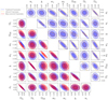Fig. 2. Predicted 2-parameter projected 1-σ and 2-σ contours on the wCDM cosmological parameters from Table 1, for Euclid. The optimistic case, probing ℓ-modes up to 5000, is considered here. The biases in the predicted values of the cosmological parameters, that arise from neglecting the basic reduced shear and magnification bias corrections, are shown here (bottom left). The additional IA-lensing bias terms are not included. Of these, Ωm, σ8, ns, ΩDE, w0, and wa have significant biases of −0.53σ, 0.43σ, −0.34σ, 1.36σ, −0.68σ, and 1.21σ, respectively. Additionally, the altered contours from including the reduced shear and magnification bias corrections, and their derivatives, in the Fisher matrix calculation are also shown (top right). The contours decrease in size for the parameters Ωb, h, ns, w0, and wa. However, in the case of ΩDE, the contours increase in size.

Furthermore, the combination of weak lensing with other probes will improve parameter constraints, whilst leaving the biases resulting from reduced shear and magnification bias unchanged; meaning that the relative biases in this scenario will be even higher. This further stresses the importance of these corrections.

4.4. The IA-enhanced lensing bias correction

When the IA-lensing bias interaction term, from Eq. (30), is also accounted for, the biases are minimally altered. These are displayed in Table 5. From these, we see that the additional term, is non-trivial, but does not induce significant biases in the cosmological parameters obtained at our current level of precision by itself. However, when combined with the basic reduced shear and magnification terms, it leads to the total bias in Ω_b becoming significant, while the total bias in n_s is suppressed to now only be on the threshold of significance. The nature of this additional correction, and its relatively minor impact, is explained by Fig. 3. This charts the change with ℓ and redshift, of the two components of the IA-enhanced lensing bias, $\delta C_{\ell ;ij}^{\mathrm{RS}+\mathrm{MB}}$ and $\delta C_{\ell ;ij}^{\mathrm{I}}$.

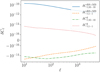Fig. 3. Two components of the IA-enhanced lensing bias correction, Eqs. (14) and (30), for the cross-spectra of our first (0.001 ≤ z ≤ 0.418), and tenth bins (1.576 ≤ z ≤ 2.50). For the first bin, the basic correction is already sub-dominant, and the additional IA-enhanced terms cancels it out. In the higher redshift bin, the second term is sub-dominant. This trend persists across all bins.

From this, we see that for the lowest redshift bins, the two already small terms cancel each other out and at higher redshifts, the latter term is evidently sub-dominant. Accordingly, while upcoming surveys must make the basic reduced shear and magnification bias corrections to extract accurate information, the IA-enhanced correction is not strictly necessary.

4.5. Forward modelling comparison

Figure 4 compares the reduced shear corrections obtained from the perturbative and forward modelling approaches, for a singular tomographic bin spanning the entire probed redshift range of 0–2.5. There is remarkable agreement between the two within the range of ℓ-modes that will be observed by Euclid, particularly at the highest and lowest ℓ-modes. We see minor disagreements at intermediate ℓ-modes, however, this is unsurprising given the various different approximations and assumptions made in the two techniques. We also note that at ℓ-modes beyond the survey’s limit, the lognormal approach will under-predict the perturbative solution. Performing cosmological inference on full forward models of the data using density-estimation likelihood-free inference (DELFI; Alsing & Wandelt 2018; Alsing et al. 2019) to compute the posteriors on cosmological parameters is emerging as a new paradigm in cosmic shear analyses (Taylor et al. 2019; Alsing & Wandelt 2018). It is shown in Taylor et al. (2019), Alsing et al. (2019) that 𝒪(1000) simulations are needed to perform inference on Stage IV data and in contrast to MCMC methods (see e.g. Foreman-Mackey et al. 2013) these can be run in parallel, at up to 100 simulations at a time. In the future it may be easier to handle the reduced shear correction in this paradigm, rather than directly computing the lensing observable with a perturbative expansion.

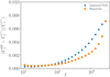Fig. 4. Reduced shear correction using the bispectrum perturbative approach (see Sect. 2.2) and using the forward model in the lognormal field approximation presented in Taylor et al. (2019). The data points are plotted at the geometric mean of the ℓ-bin boundaries. There is mild disagreement at intermediate ℓ-modes. This is to be expected given the approximations that go into the bispectrum fitting formula and the lognormal field approximation. Nevertheless the agreement at low-ℓ and in the highest ℓ-bin are striking. Here $C_{\mathcal{l}}^{gg}$ labels the reduced shear auto-correlation spectrum, while $C_{\mathcal{l}}^{\gamma \gamma }$ denotes the shear-shear auto-correlation spectrum.

The eventual aim for a DELFI pipeline (Taylor et al. 2019) is to compute lensing observables from full N-body simulations (see e.g. Izard et al. 2017). This would avoid the need to write a matter bispectrum emulator trained on simulations, although, the N-body simulations used for this purpose would need to accurately represent the physics of the bispectrum.

5. Conclusions

In this work, we quantified the impact that making the reduced shear approximation and neglecting magnification bias will have on angular power spectra of upcoming weak lensing surveys. Specifically, we calculated the biases that would be expected in the cosmological parameters obtained from Euclid. By doing so, significant biases were found for Ω_m, σ₈, n_s, Ω_DE, w₀, and w_a of −0.53σ, 0.43σ, −0.34σ, 1.36σ, −0.68σ, and 1.21σ, respectively. We also built the formalism for an IA-enhanced correction. This was discovered to be sub-dominant. Given the severity of our calculated biases, we conclude that it is necessary to make both the reduced shear and magnification bias corrections for Stage IV experiments.

However, there are important limitations to consider in the approach described here. In calculating these corrections, the Limber approximation is still made. This approximation is typically valid above ℓ ∼ 100. But, for Euclid we expect to reach ℓ-modes of ten. Therefore, the impact of this simplification at the correction level must be evaluated. Given that the dominant contributions to the reduced shear and magnification bias corrections come from ℓ-modes above 100, we would not expect the Limber approximation to significantly affect the resulting cosmological biases. However, an explicit calculation is still warranted. Furthermore, the various correction terms depend on bispectra which are not well understood: they both involve making a plethora of assumptions, and using fitting formulae that have accuracies of only 30–50% on small scales.

In addition, this work does not consider the impact of baryonic feedback on the corrections. We would expect that baryonic feedback behaves in a similar way to lowering the fiducial value σ₈ (see Appendix C), that is, they both suppress structure growth in high density regions. Accordingly, it is likely that the inclusion of baryonic feedback would have an effect on these corrections. If the matter power spectrum is suppressed by a greater fraction than the matter bispectrum, then the biases will increase. However, it is not currently clear to what degree the matter bispectrum is suppressed relative to the matter power spectrum, and existing numerical simulations propose seemingly inconsistent answers (see e.g. Barreira et al. 2019 in comparison to Semboloni et al. 2013). For this reason, we cannot robustly quantify the impact of baryonic feedback on the biases. As knowledge of the impact of baryons on the bispectrum improves, the reduced shear and magnification bias corrections should be modified accordingly.

An additional hurdle is the large computational expense of these terms; arising from the multiple nested integrals needing numerical computation. Computing the reduced shear and magnification bias corrections for this work took of the order of 24 h when multiprocessing across 100 CPU threads. Including the IA-enhanced correction term increases this to ∼48 h. This expense can be prohibitive if the correction is to be included in inference methods. Considering that forward modelling approaches, such as a DELFI pipeline, could both bypass the need for matter bispectrum fitting formulae, and reduce computation time, we recommend that forward modelling should be used to account for these corrections in the future. However, there is also merit in exploring whether the existing processes can be optimised.

Acknowledgments

We thank the anonymous referee for their constructive comments, and Paniez Paykari for her programming expertise. ACD and TDK are supported by the Royal Society. PLT acknowledges support for this work from a NASA Postdoctoral Program Fellowship and the UK Science and Technologies Facilities Council. Part of the research was carried out at the Jet Propulsion Laboratory, California Institute of Technology, under a contract with the National Aeronautics and Space Administration. The Euclid Consortium acknowledges the European Space Agency and the support of a number of agencies and institutes that have supported the development of Euclid, in particular the Academy of Finland, the Agenzia Spaziale Italiana, the Belgian Science Policy, the Canadian Euclid Consortium, the Centre National d’Etudes Spatiales, the Deutsches Zentrum für Luft- und Raumfahrt, the Danish Space Research Institute, the Fundação para a Ciência e a Tecnologia, the Ministerio de Economia y Competitividad, the National Aeronautics and Space Administration, the Netherlandse Onderzoekschool Voor Astronomie, the Norwegian Space Agency, the Romanian Space Agency, the State Secretariat for Education, Research and Innovation (SERI) at the Swiss Space Office (SSO), and the United Kingdom Space Agency. A detailed complete list is available on the Euclid web site (http://www.euclid-ec.org).

References

Appendix A: Generalised lensing bispectra formulae

We can extend the methodology used to describe the matter bispectrum, B_δδδ, to describe the bispectrum of three related quantities, B_μνη. Here, the three fields μ, ν, and η are proportional to the density contrast, δ, by some redshift-dependent weightings. This means they behave as δ would, under a small change in the fiducial cosmology. In this way, the second-order perturbation theory approach of Fry (1984) remains valid. We also assume Gaussian random initial conditions. Accordingly, the bispectrum is defined by first and second-order terms:

$$\begin{array}{cc}& B_{\mu \nu \eta }({\mathit{k}}_1,{\mathit{k}}_2,{\mathit{k}}_3)=⟨[{\stackrel{\sim }{\mu }}^{(1)}({\mathit{k}}_1)+{\stackrel{\sim }{\mu }}^{(2)}({\mathit{k}}_1)]\hfill \\ \hfill & \times [{\stackrel{\sim }{\nu }}^{(1)}({\mathit{k}}_2)+{\stackrel{\sim }{\nu }}^{(2)}({\mathit{k}}_2)]\hfill \\ \hfill & \times [{\stackrel{\sim }{\eta }}^{(1)}({\mathit{k}}_3)+{\stackrel{\sim }{\eta }}^{(2)}({\mathit{k}}_3)]⟩,\hfill \end{array}$$(A.1)

where the superscripts (2) and (1) denote the second and first-order terms respectively. But because we take Gaussian random initial conditions, the value of the three-point correlation vanishes at the lowest-order. Additionally, we can neglect products of second-order terms, as these are fourth-order terms. Equation (A.1) now becomes:

$$\begin{array}{cc}& B_{\mu \nu \eta }({\mathit{k}}_1,{\mathit{k}}_2,{\mathit{k}}_3)=⟨{\stackrel{\sim }{\mu }}^{(2)}({\mathit{k}}_1){\stackrel{\sim }{\nu }}^{(1)}({\mathit{k}}_2){\stackrel{\sim }{\eta }}^{(1)}({\mathit{k}}_3)⟩\hfill \\ \hfill & +⟨{\stackrel{\sim }{\nu }}^{(2)}({\mathit{k}}_2){\stackrel{\sim }{\mu }}^{(1)}({\mathit{k}}_1){\stackrel{\sim }{\eta }}^{(1)}({\mathit{k}}_3)⟩\hfill \\ \hfill & +⟨{\stackrel{\sim }{\eta }}^{(2)}({\mathit{k}}_3){\stackrel{\sim }{\mu }}^{(1)}({\mathit{k}}_1){\stackrel{\sim }{\nu }}^{(1)}({\mathit{k}}_2)⟩.\hfill \end{array}$$(A.2)

The above assumption relating the three fields to δ, also leads us to concluding that δ⁽¹⁾ is related to δ⁽²⁾ in the same way that μ⁽¹⁾, ν⁽¹⁾, and η⁽¹⁾ are related to μ⁽²⁾, ν⁽²⁾, and η⁽²⁾ respectively. In which case, we can directly adapt Eq. (40) of Fry (1984), to read:

$$\begin{array}{cc}& B_{\mu \nu \eta }({\mathit{k}}_1,{\mathit{k}}_2,{\mathit{k}}_3)=2F_2({\mathit{k}}_2,{\mathit{k}}_3)P_{\mu \nu }({\mathit{k}}_2)P_{\mu \eta }({\mathit{k}}_3)\hfill \\ \hfill & +2F_2({\mathit{k}}_1,{\mathit{k}}_3)P_{\nu \mu }({\mathit{k}}_1)P_{\nu \eta }({\mathit{k}}_3)\hfill \\ \hfill & +2F_2({\mathit{k}}_1,{\mathit{k}}_2)P_{\eta \mu }({\mathit{k}}_1)P_{\eta \nu }({\mathit{k}}_2),\hfill \end{array}$$(A.3)

with:

$$\begin{array}{c}\hfill F_2({\mathit{k}}_1,{\mathit{k}}_2)=\frac{5}{7}+\frac{1}{2}\frac{{\mathit{k}}_1·{\mathit{k}}_2}{k_1{k}_2}(\frac{k_1}{k_2}+\frac{k_2}{k_1})+\frac{2}{7}(\frac{{\mathit{k}}_1·{\mathit{k}}_2}{k_1{k}_2}{)}^2.\end{array}$$(A.4)

As in Scoccimarro & Couchman (2001), this can then be modified to include numerical fitting to N-body simulations by exchanging F₂ for $F_2^{\text{eff}}$, as defined in Eq. (17). The fitting formula determined in Scoccimarro & Couchman (2001) still remains valid, because it does not have any redshift dependence and does not depend on the fiducial cosmology. The density perturbation-IA bispectrum, used in the IA-enhanced lensing bias correction, is then a specific case of this formula, where μ = ν = δ, and η = I.

Appendix B: The “pessimistic” case for Euclid

Given the complexities of modelling both astrophysical uncertainties and the non-Gaussian covariance terms at high ℓ-modes, Euclid Collaboration et al. (2019) define a “pessimistic” case for Euclid forecasts. In this case, an ℓ-cut is made at 1500. In this section, we calculate the uncertainties on the cosmological parameters, and the biases induced in them by the reduced shear approximation and magnification when this cut is made. Here, as before, we include both the Gaussian and SSC covariance terms. The results are shown in Table B.1.

Now, we find that the biases are significantly reduced in comparison to the “optimistic” case. However, the bias in Ω_DE remains significant, at 0.28σ. Therefore, even in this non-ideal scenario, the reduced shear and magnification bias corrections must still be made.

Appendix C: The impact of varying the fiducial cosmology

Owing to the fact that the reduced shear and magnification bias corrections are a projection of the matter bispectrum, while the shear auto and cross-spectra are projections of the matter power spectrum, the relative size of the correction in comparison to the shear spectra is strongly influenced by non-linearity (Shapiro 2009). The parameters σ₈ and n_s have the strongest effect on non-linearity, therefore we examine the effect of changing these parameters on the biases, assuming a Gaussian covariance.

Tables C.1 and C.2 show the recomputed uncertainties and biases, respectively, when the fiducial values of σ₈ are lowered to 0.716, and raised to 0.916. These biases are also visualised in Fig. C.1. As expected, lowering the fiducial value of σ₈ suppresses the biases, though they still remain significant, whilst raising this value aggravates the biases. Contributing to these changes is also the fact that the predicted uncertainties in the parameters generally decrease as σ₈ is increased, with the exception of σ₈ itself.

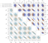Fig. C.1. Predicted 1- and 2-σ contours on the wCDM cosmological parameters, for Euclid, for different values of σ8. All other parameter values are fixed to those shown in Table 1. Confidence regions and biases for σ8 = 0.716 (bottom left), and σ8 = 0.916 (top right) are shown. The additional IA-enhanced lensing bias is not included in these results. For the lower value of σ8, the biases are supressed slightly, but still remain significant. However, for the higher value of σ8, the significances of the biases in the cosmological parameters are heightened.

The effects on the uncertainties of varying n_s, to 0.86 then 1.06, are shown in Table C.1. Figure C.2 and Table C.2 show the biases after this variation. The effect on the significances of the biases is less straightforward in this case. The parameters are affected relatively differently in comparison to the variation of σ₈. In general, the change in the ratio of the biases to the uncertainties is non-trivial, but relatively subtle. The exceptions to this being σ₈ and Ω_m. For these parameters, the biases reduce considerably in magnitude. Despite the changes, the biases in each of the previously affected parameters remain significant.

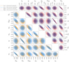Fig. C.2. Predicted 1- and 2-σ contours on the wCDM cosmological parameters, for Euclid, for different values of ns. All other parameter values are fixed to those shown in Table 1. Confidence regions and biases for ns = 0.86 (bottom left), and ns = 1.06 (top right) are shown. The additional IA-enhanced lensing bias is not included in these results. In general, varying the fiducial value of ns does not cause notable change to the significances of the biases.

All Tables

All Figures

Fig. 1. Reduced shear (top left), magnification bias (top right), and combined (bottom) corrections relative to the observed angular shear auto-correlation spectra (excluding shot noise), for four different redshift bins. For the basic reduced shear correction, the relative size of the correction increases alongside redshift, as the correction term has an additional factor of the lensing kernel compared to the power spectra. The correction plateaus at higher redshifts, because the lensed light encounters the most non-linearity and clustering at lower redshifts. It also increases with ℓ, as convergence tends to be higher on smaller physical scales. For the basic magnification bias correction, the relative size of the correction also increases with redshift. At lower redshifts, the term is subtractive, as the magnification of individual galaxies dominates, leading to an overestimation of the galaxy density. Whereas, at higher redshifts, the dilution of galaxy density dominates, leading to an underestimation of the power spectra if the correction is not made. For the combined effect of the two corrections, the magnification bias correction effectively cancels out the reduced shear correction at the lowest redshifts. Meanwhile, at intermediate redshifts, the magnification bias is small, but additive; slightly enhancing the reduced shear correction. However, at the highest redshifts, the magnification bias is particularly strong, and the combined correction is significantly greater than at lower redshifts. The corrections seen here are in the case of the wCDM cosmology of Table 1.

In the text

Fig. 2. Predicted 2-parameter projected 1-σ and 2-σ contours on the wCDM cosmological parameters from Table 1, for Euclid. The optimistic case, probing ℓ-modes up to 5000, is considered here. The biases in the predicted values of the cosmological parameters, that arise from neglecting the basic reduced shear and magnification bias corrections, are shown here (bottom left). The additional IA-lensing bias terms are not included. Of these, Ωm, σ8, ns, ΩDE, w0, and wa have significant biases of −0.53σ, 0.43σ, −0.34σ, 1.36σ, −0.68σ, and 1.21σ, respectively. Additionally, the altered contours from including the reduced shear and magnification bias corrections, and their derivatives, in the Fisher matrix calculation are also shown (top right). The contours decrease in size for the parameters Ωb, h, ns, w0, and wa. However, in the case of ΩDE, the contours increase in size.

In the text

	Fig. 3. Two components of the IA-enhanced lensing bias correction, Eqs. (14) and (30), for the cross-spectra of our first (0.001 ≤ z ≤ 0.418), and tenth bins (1.576 ≤ z ≤ 2.50). For the first bin, the basic correction is already sub-dominant, and the additional IA-enhanced terms cancels it out. In the higher redshift bin, the second term is sub-dominant. This trend persists across all bins.
In the text

Fig. 4. Reduced shear correction using the bispectrum perturbative approach (see Sect. 2.2) and using the forward model in the lognormal field approximation presented in Taylor et al. (2019). The data points are plotted at the geometric mean of the ℓ-bin boundaries. There is mild disagreement at intermediate ℓ-modes. This is to be expected given the approximations that go into the bispectrum fitting formula and the lognormal field approximation. Nevertheless the agreement at low-ℓ and in the highest ℓ-bin are striking. Here $C_{\mathcal{l}}^{gg}$ labels the reduced shear auto-correlation spectrum, while $C_{\mathcal{l}}^{\gamma \gamma }$ denotes the shear-shear auto-correlation spectrum.

In the text

Fig. C.1. Predicted 1- and 2-σ contours on the wCDM cosmological parameters, for Euclid, for different values of σ8. All other parameter values are fixed to those shown in Table 1. Confidence regions and biases for σ8 = 0.716 (bottom left), and σ8 = 0.916 (top right) are shown. The additional IA-enhanced lensing bias is not included in these results. For the lower value of σ8, the biases are supressed slightly, but still remain significant. However, for the higher value of σ8, the significances of the biases in the cosmological parameters are heightened.

In the text

Fig. C.2. Predicted 1- and 2-σ contours on the wCDM cosmological parameters, for Euclid, for different values of ns. All other parameter values are fixed to those shown in Table 1. Confidence regions and biases for ns = 0.86 (bottom left), and ns = 1.06 (top right) are shown. The additional IA-enhanced lensing bias is not included in these results. In general, varying the fiducial value of ns does not cause notable change to the significances of the biases.

In the text

References

- Akeson, R., Armus, L., & Bachelet, E. 2019, ArXiv e-prints [arXiv:1902.05569] [Google Scholar]
- Albrecht, A., Bernstein, G., Cahn, R., et al. 2006, ArXiv e-prints [arXiv:astro-ph/0609591] [Google Scholar]
- Alsing, J., Charnock, T., Feeney, S., & Wandelt, B. 2019, MNRAS, 488, 4440 [NASA ADS] [CrossRef] [Google Scholar]
- Alsing, J., & Wandelt, B. 2018, MNRAS, 476, L60 [NASA ADS] [CrossRef] [Google Scholar]
- Bacon, D., Refregier, A., & Ellis, R. 2000, MNRAS, 318, 625 [NASA ADS] [CrossRef] [Google Scholar]
- Barreira, A., Krause, E., & Schmidt, F. 2018, J. Cosmology Astropart. Phys., 2018, 053 [Google Scholar]
- Barreira, A., Nelson, D., Pillepich, A., et al. 2019, MNRAS, 488, 2079 [NASA ADS] [CrossRef] [Google Scholar]
- Blake, C., & Bridle, S. 2005, MNRAS, 363, 1329 [NASA ADS] [CrossRef] [Google Scholar]
- Blas, D., Lesgourgues, J., & Tram, T. 2011, J. Cosmology Astropart. Phys., 2011, 034 [Google Scholar]
- Bridle, S., & King, L. 2007, New J. Phys., 9, 444 [NASA ADS] [CrossRef] [Google Scholar]
- Cropper, M., Cole, R., James, A., et al. 2012, Proc. SPIE, 8442, 84420V [Google Scholar]
- Dark Energy Survey Collaboration 2005, ArXiv e-prints [arXiv:astro-ph/0510346] [Google Scholar]
- Dodelson, S., Shapiro, C., & White, M. 2006, Phys. Rev. D, 73, 023009 [NASA ADS] [CrossRef] [Google Scholar]
- Duncan, C. A. J., Joachimi, B., Heavens, A. F., Heymans, C., & Hildebrandt, H. 2014, MNRAS, 437, 2471 [NASA ADS] [CrossRef] [Google Scholar]
- Euclid Collaboration (Blanchard, A., et al.) 2019, A&A, submitted [arXiv:1910.09273] [Google Scholar]
- Foreman-Mackey, D., Hogg, D. W., Lang, D., & Goodman, J. 2013, PASP, 125, 306 [CrossRef] [Google Scholar]
- Fry, J. 1984, ApJ, 279, 499 [NASA ADS] [CrossRef] [Google Scholar]
- Górski, K. M., Wandelt, B. D., Hansen, F. K., Hivon, E., & Banday, A. J. 1999, ArXiv e-prints [arXiv: astro-ph/9905275] [Google Scholar]
- Górski, K. M., Hivon, E., Banday, A. J., et al. 2005, ApJ, 622, 759 [NASA ADS] [CrossRef] [Google Scholar]
- Heymans, C., Van Waerbeke, L., Miller, L., et al. 2012, MNRAS, 427, 146 [NASA ADS] [CrossRef] [Google Scholar]
- Hilbert, S., Hartlap, J., & Schneider, P. 2011, A&A, 536, A85 [NASA ADS] [CrossRef] [EDP Sciences] [Google Scholar]
- Hildebrandt, H., Viola, M., Heymans, C., et al. 2017, MNRAS, 465, 1454 [Google Scholar]
- Hu, W., & Kravtsov, A. V. 2003, ApJ, 584, 702 [NASA ADS] [CrossRef] [Google Scholar]
- Hui, L., Gaztañaga, E., & Loverde, M. 2007, Phys. Rev. D, 76, 103502 [NASA ADS] [CrossRef] [Google Scholar]
- Izard, A., Fosalba, P., & Crocce, M. 2017, MNRAS, 473, 3051 [NASA ADS] [CrossRef] [Google Scholar]
- Joachimi, B., & Bridle, S. L. 2010, A&A, 523, A1 [NASA ADS] [CrossRef] [EDP Sciences] [Google Scholar]
- Joachimi, B., Cacciato, M., Kitching, T., et al. 2015, Space Sci. Rev., 193, 1 [NASA ADS] [CrossRef] [Google Scholar]
- Kaiser, N., Wilson, G., & Luppino, G. A. 2000, ArXiv e-prints [arXiv:astro-ph/0003338] [Google Scholar]
- Kiessling, A., Cacciato, M., Joachimi, B., et al. 2015, Space Sci. Rev., 193, 67 [NASA ADS] [CrossRef] [Google Scholar]
- Kilbinger, M. 2015, Rep. Prog. Phys., 78, 086901 [Google Scholar]
- Kilbinger, M., Heymans, C., Asgari, M., et al. 2017, MNRAS, 472, 2126 [NASA ADS] [CrossRef] [Google Scholar]
- Kirk, D., Brown, M., Hoekstra, H., et al. 2015, Space Sci. Rev., 193, 139 [NASA ADS] [CrossRef] [Google Scholar]
- Kitching, T. D., Alsing, J., Heavens, A. F., et al. 2017, MNRAS, 469, 2737 [NASA ADS] [CrossRef] [Google Scholar]
- Kitching, T. D., & Heavens, A. F. 2017, Phys. Rev. D, 95, 063522 [NASA ADS] [CrossRef] [Google Scholar]
- Krause, E., & Hirata, C. 2010, A&A, 523, A28 [NASA ADS] [CrossRef] [EDP Sciences] [Google Scholar]
- Lacasa, F., & Grain, J. 2019, A&A, 624, A61 [NASA ADS] [CrossRef] [EDP Sciences] [Google Scholar]
- Laureijs, R., Amiaux, J., Arduini, S., et al. 2011, ArXiv e-prints [arXiv:1110.3193] [Google Scholar]
- Lewis, A., Challinor, A., & Lasenby, A. 2000, ApJ, 538, 473 [NASA ADS] [CrossRef] [Google Scholar]
- Lin, C. H., Harnois-Déraps, J., Eifler, T., et al. 2019, MNRAS, submitted [arXiv:1905.03779] [Google Scholar]
- Liu, J., Haiman, Z., Hui, L., Kratochvil, J. M., & May, M. 2014, Phys., 89, 023515 [Google Scholar]
- Lorenz, C. S., Alonso, D., & Ferreira, P. G. 2018, Phys. Rev. D, 97, 023537 [NASA ADS] [CrossRef] [Google Scholar]
- LSST Science Collaboration (Abell, P. A., et al.) 2009, ArXiv e-prints [arXiv:0912.0201] [Google Scholar]
- Mancini, A. S., Taylor, P., Reischke, R., et al. 2018, Phys. Rev D, 98, 103507 [NASA ADS] [CrossRef] [Google Scholar]
- Massey, R., Hoekstra, H., Kitching, T., et al. 2013, MNRAS, 429, 661 [Google Scholar]
- Rhodes, J., Refregier, A., & Groth, E. J. 2000, ApJ, 536, 79 [NASA ADS] [CrossRef] [Google Scholar]
- Rudd, D., Zentner, A., & Kravtsov, A. 2008, ApJ, 672, 19 [NASA ADS] [CrossRef] [Google Scholar]
- Schmidt, F., Rozo, E., Dodelson, S., Hui, L., & Sheldon, E. 2009, ApJ, 702, 593 [NASA ADS] [CrossRef] [Google Scholar]
- Scoccimarro, R., & Couchman, H. 2001, MNRAS, 325, 1312 [NASA ADS] [CrossRef] [Google Scholar]
- Sellentin, E., & Starck, J. 2019, J. Cosmol. Astropart. Phys., 8, 21 [Google Scholar]
- Sellentin, E., Heymans, C., & Harnois-Déraps, J. 2018, MNRAS, 477, 4879 [NASA ADS] [CrossRef] [Google Scholar]
- Semboloni, E., Hoekstra, H., & Schaye, J. 2013, MNRAS, 434, 148 [NASA ADS] [CrossRef] [Google Scholar]
- Shapiro, C. 2009, ApJ, 696, 775 [NASA ADS] [CrossRef] [EDP Sciences] [Google Scholar]
- Smith, R., Peacock, J., Jenkins, A., et al. 2003, MNRAS, 341, 1311 [NASA ADS] [CrossRef] [Google Scholar]
- Takada, M., & Hu, W. 2013, Phys. Rev. D, 87, 123504 [NASA ADS] [CrossRef] [Google Scholar]
- Takahashi, R., Sato, M., Nishimichi, T., Taruya, A., & Oguri, M. 2012, ApJ, 761, 152 [NASA ADS] [CrossRef] [Google Scholar]
- Taylor, A., Kitching, T., Bacon, D., & Heavens, A. 2007, MNRAS, 374, 1377 [NASA ADS] [CrossRef] [Google Scholar]
- Taylor, P. L., Kitching, T. D., Alsing, J., et al. 2019, Phys. Rev. D, 100, 023519 [NASA ADS] [CrossRef] [Google Scholar]
- Taylor, P. L., Kitching, T. D., McEwen, J. D., & Tram, T. 2018, Phys. Rev. D, 98, 023522 [NASA ADS] [CrossRef] [Google Scholar]
- Tegmark, M., Taylor, A., & Heavens, A. 2015, ApJ, 78, 086901 [Google Scholar]
- Thiele, L., Duncan, C. A. J., & Alonso, D. 2020, MNRAS, 491, 1746 [NASA ADS] [CrossRef] [Google Scholar]
- Troxel, M. A., MacCrann, N., Zuntz, J., et al. 2018, Phys. Rev. D, 98, 043528 [NASA ADS] [CrossRef] [Google Scholar]
- Turner, E. L., Ostriker, J. P., & Gott, J. R., III 1984, ApJ, 284, 1 [NASA ADS] [CrossRef] [Google Scholar]
- Van Waerbeke, L., Benjamin, J., Erben, T., et al. 2013, MNRAS, 433, 3373 [Google Scholar]
- Van Waerbeke, L., Mellier, Y., Erben, T., et al. 2000, A&A, 358, 30 [NASA ADS] [Google Scholar]
- Wittman, D., Tyson, J., Kirkman, D., Dell’Antonio, I., & Bernstein, G. 2000, Nature, 405, 143 [NASA ADS] [CrossRef] [PubMed] [Google Scholar]
- Xavier, H. S., Abdalla, F. B., & Joachimi, B. 2016, MNRAS, 459, 3693 [NASA ADS] [CrossRef] [Google Scholar]
- Zuntz, J., Paterno, M., Jennings, E., et al. 2015, Astron. Comput., 12, 45 [NASA ADS] [CrossRef] [Google Scholar]