| Issue |
A&A
Volume 657, January 2022
|
|
|---|---|---|
| Article Number | A123 | |
| Number of page(s) | 11 | |
| Section | Galactic structure, stellar clusters and populations | |
| DOI | https://doi.org/10.1051/0004-6361/202141596 | |
| Published online | 21 January 2022 | |
Precise distances from OGLE-IV member RR Lyrae stars in six bulge globular clusters⋆
1
Universidade de São Paulo, IAG, Rua do Matão 1226, Cidade Universitária, São Paulo 05508-900, Brazil
e-mail: This email address is being protected from spambots. You need JavaScript enabled to view it.
2
Università di Padova, Dipartimento di Fisica e Astronomia, Vicolo dell’Osservatorio 2, 35122 Padova, Italy
3
INAF-Osservatorio Astronomico di Padova, Vicolo dell’Osservatorio 5, 35122 Padova, Italy
4
Centro di Ateneo di Studi e Attività Spaziali “Giuseppe Colombo” – CISAS, Via Venezia 15, 35131 Padova, Italy
5
Universidade Estadual de Santa Cruz, Rodovia Jorge Amado km 16, Ilhéus 45662-000, Brazil
6
Universidade Federal do Rio de Janeiro, Av. Athos da Silveira, 149, Cidade Universitária, Rio de Janeiro 21941-909, Brazil
7
Universidade Federal do Rio Grande do Sul, Departamento de Astronomia, CP 15051, Porto Alegre 91501-970, Brazil
8
INAF – Astronomical Observatory of Abruzzo, Via M. Maggini, sn, 64100 Teramo, Italy
9
INFN – Sezione di Pisa, Largo Pontecorvo 3, 56127 Pisa, Italy
10
Instituto de Astronomía, Universidad Nacional Autónoma de México, A.P. 106, 22800 Ensenada, B.C., México
Received:
19
June
2021
Accepted:
6
October
2021
Abstract
Context. RR Lyrae stars are useful standard candles allowing one to derive accurate distances for old star clusters. Based on the recent catalogues from OGLE-IV and Gaia Early Data Release 3 (EDR3), the distances can be improved for a few bulge globular clusters.
Aims. The aim of this work is to derive an accurate distance for the following six moderately metal-poor, relatively high-reddening bulge globular clusters: NGC 6266, NGC 6441, NGC 6626, NGC 6638, NGC 6642, and NGC 6717.
Methods. We combined newly available OGLE-IV catalogues of variable stars containing mean I magnitudes, with Clement’s previous catalogues containing mean V magnitudes, and with precise proper motions from Gaia EDR3. Astrometric membership probabilities were computed for each RR Lyrae, in order to select those compatible with the cluster proper motions. Applying luminosity–metallicity relations derived from BaSTI α-enhanced models (He-enhanced for NGC 6441 and canonical He for the other clusters), we updated the distances with relatively low uncertainties.
Results. Distances were derived with the I and V bands, with a 5 − 8% precision. We obtained 6.6 kpc, 13.1 kpc, 5.6 kpc, 9.6 kpc, 8.2 kpc, and 7.3 kpc for NGC 6266, NGC 6441, NGC 6626, NGC 6638, NGC 6642, and NGC 6717, respectively. The results are in excellent agreement with the literature for all sample clusters, considering the uncertainties.
Conclusions. The present method of distance derivation, based on recent data of member RR Lyrae stars, updated BaSTI models, and robust statistical methods, proved to be consistent. A larger sample of clusters will be investigated in a future work.
Key words: stars: variables: RR Lyrae / globular clusters: general / Galaxy: bulge
Catalogue is only available at the CDS via anonymous ftp to cdsarc.u-strasbg.fr (130.79.128.5) or via http://cdsarc.u-strasbg.fr/viz-bin/cat/J/A+A/657/A123
© ESO 2022
1. Introduction
Globular clusters (GCs) in the Galactic bulge are important tracers of the early history of the Galaxy formation (e.g., Barbuy et al. 2018), as they keep a memory of the evolution of the Galaxy. Distances of GCs are the most uncertain information in their studies in terms of Galaxy structure, stellar population components, and calculation of orbits (Bica et al. 2006). In particular, the orbital parameters of the clusters projected towards the Milky Way (MW) bulge and their membership to different Galactic regions are very sensitive to the assumed heliocentric and Galactocentric distances (e.g., Pérez-Villegas et al. 2020).
These distances and the membership to the bulge region are also of great interest in the study of high-energy sources since closer distances imply higher stellar densities and possibly a greater occurrence of such sources (Ortolani et al. 2007). Several bulge GCs host a significant number of X-ray sources and millisecond pulsars. The most interesting case is Terzan 5, which contains 39 pulsars (Ransom et al. 2005; Cadelano et al. 2018), that is 25% of all pulsars in MW GCs. Heinke et al. (2006) detected 50 X-ray sources with Chandra data. The distance of Terzan 5 was derived in Ortolani et al. (2007) by comparing the horizontal branch (HB) level relative to the reddening lines over the HB of the template cluster NGC 6528, using NICMOS and SOFI near-infrared (NIR) photometry.
RR Lyrae stars (RRLs) are radially pulsating stars, characteristic of metal-poor, old (Population II) stellar populations. With periods ranging from 0.2 to 1.0 days, these variable stars are more commonly found on the instability strip of metal-poor GCs ([Fe/H] ≲ −0.8). Assuming metallicity and reddening values for Galactic GCs, the cluster distances can be precisely derived with well-calibrated period–luminosity and luminosity–metallicity relations (e.g., Gaia Collaboration 2017; Muhie et al. 2021). The combination of the absolute magnitudes with the mean magnitudes of the RRLs, observed with time-series photometry, makes them useful standard candles.
In this work, we derive accurate distances for the bulge GCs NGC 6266, NGC 6441, NGC 6626, NGC 6638, NGC 6642, and NGC 6717, for which new data of the fourth release of the Optical Gravitational Lensing Experiment (OGLE-IV) survey revealed larger samples of RRLs (Soszyński et al. 2019). These six moderately metal-poor GCs are within the selection of bulge GCs by Bica et al. (2016), and they are located in the direction of the Galactic centre (RGC < 4.0 kpc), with a relatively high foreground reddening of E(B − V)∼0.40.
In addition to the high stellar crowding present in the bulge, the high total and differential extinctions hamper the distance derivation through isochrone fitting even more since they produce a non-uniform spread in colour-magnitude diagrams (CMDs; e.g., Alonso-García et al. 2011). These effects are mitigated when going to redder wavelengths, such as the I or near-infrared bands, for which AI/AV ∼ 0.60 and AKS/AV ∼ 0.12 (e.g., Ortolani et al. 2019; Kerber et al. 2019). In particular for the study of RRLs, the I filter gives the best compromise between spatial resolution and light curve amplitude, which is around 0.3 − 0.8 mag (compared to 0.5 − 1.0 mag for the V filter). For this reason, the mean I magnitudes provided by the new data from OGLE-IV (Soszyński et al. 2019) greatly contribute to complete the census of RRLs in bulge GCs.
In order to gather the relevant data on the RRLs of the sample clusters, we cross-matched the recent catalogues of RRLs from OGLE-IV with the earlier catalogues from Clement et al. (2001, 2017 edition) and Gaia Data Release 2 (DR2; Gaia Collaboration 2016b, 2018). We also cross-identified the RRLs with the absolute proper motions (PMs) from Gaia Early Data Release 3 (EDR3; Gaia Collaboration 2021a), and assigned a membership probability to select a reliable sample of cluster RRLs. These data allow one to update globular cluster distances with a relatively high accuracy and better constrain the free parameters contained in an isochrone fitting (e.g., Kerber et al. 2019; Oliveira et al. 2020; Souza et al. 2020). This approach based on member RRLs is not affected as the isochrone fitting techniques by the problems of binarity, field contamination, and distortion of the CMD due to the dependence of reddening correction on the stellar effective temperature, which can dramatically hamper the possibility to obtain reliable distances of very reddened, low Galactic latitude clusters.
It is worth noting that NGC 6266, NGC 6441, and NGC 6626 host: seven, six and 14 pulsars1, respectively. In this sense, a precise age and distance derivation for these GCs have a crucial importance, since their distances can be used to compute stellar densities and stellar interaction rates (Ortolani et al. 2007).
A recent effort on distance derivation from Gaia DR2 PMs and radial velocities was carried out in Baumgardt et al. (2019), where they calculated the kinematic distances of 154 GCs by fitting N-body models with a maximum-likelihood approach. Comparing their findings with Harris (1996, 2010 edition2, hereafter H10) and Watkins et al. (2015), they found a good agreement for distances up to ∼7 kpc, but derived systematic 10% higher distances beyond it. More recently, Vasiliev & Baumgardt (2021) and Baumgardt & Vasiliev (2021) derived distances from Gaia EDR3 parallaxes, velocity dispersion profiles, and stellar counts, and they compared them to an average of literature distances. For our sample, the average resulted in 6.41 kpc, 12.73 kpc, 5.37 kpc, 9.78 kpc, 8.05 kpc, and 7.52 kpc, whereas the parallaxes resulted in 5.55 kpc, 12.66 kpc, 5.10 kpc, 9.01 kpc, 8.26 kpc, 8.85 kpc for NGC 6266, NGC 6441, NGC 6626, NGC 6638, NGC 6642, and NGC 6717, respectively.
Several literature works on these GCs used the distances from H10 as input parameters, using in turn an average of the VHB magnitudes measured in the literature with isochrone fitting methods as a distance indicator. In the case of NGC 6266, H10 reports the VHB from Brocato et al. (1996), who give 6.8 kpc. Following works derived slightly different distances: 6.95 kpc (Ferraro et al. 1999); 6.64 ± 0.51 kpc (Beccari et al. 2006); 6.67 ± 0.44 kpc (Contreras et al. 2010); 7.05 ± 0.58 kpc (McNamara & McKeever 2011); and 6.42 ± 0.14 kpc (Watkins et al. 2015). For a long time, NGC 6266 has been known to host several RRLs (Bailey 1902; van Agt & Oosterhoff 1959), and most of them were discovered by Contreras et al. (2010), placing it as the second cluster with the highest number of RRLs, only below NGC 5272.
Despite its high metallicity (Rich et al. 1997), the dense cluster NGC 6441 contains an extended blue HB with a sizable population of peculiar RRL stars. For this cluster, H10 reported a distance of 10.4 − 11.9 kpc from Pritzl et al. (2001), and the following works have provided 13.5 kpc from SOFI@NTT NIR data (Valenti et al. 2007), 13.61 kpc from a K-band period–luminosity–metallicity relation (Dall’Ora et al. 2008), and 13.0 kpc from VVV NIR data of RRLs (Alonso-García et al. 2021). Apart from the strong differential reddening in the bulge region, this discrepancy can be explained by an overabundance of He which is usually neglected, as discussed in Alonso-García et al. (2021).
For NGC 6626 (M28), H10 reported the HB magnitude from Testa et al. (2001) as VHB = 15.55 ± 0.10 (close to 15.5 from Davidge et al. 1996), a distance of 5.5 kpc. Recently, Kerber et al. (2018) derived a distance of 5.34 ± 0.21 kpc by applying statistical isochrone fitting to HST proper-motion-cleaned CMDs, and Alonso-García et al. (2021) derived 5.41 kpc. For NGC 6638, H10 reported a distance of 9.4 kpc from Piotto et al. (2002), which was derived with HST/WFPC2 photometry. Valenti et al. (2005) obtained 10.33 kpc from SOFI NIR data, coherent with the results from Baumgardt & Vasiliev (2021).
For NGC 6642, H10 reported 8.1 kpc from Piotto et al. (2002). Other works derived the following: 7.2 ± 0.5 kpc using SOAR BVI photometry (Barbuy et al. 2006); 8.63 kpc from SOFI NIR data (Valenti et al. 2007); and 8.05 ± 0.66 kpc from HST/ACS photometry (Balbinot et al. 2009). Finally, for NGC 6717, H10 reported 7.1 kpc from Ortolani et al. (1999), which was derived with BV photometry from the Danish telescope. With HST/ACS data and different isochrones, Dotter et al. (2010) and VandenBerg et al. (2013) obtained 7.55 kpc and 7.27 kpc. Very recently, Oliveira et al. (2020) derived 7.33 ± 0.12 kpc from HST data, by applying a statistical isochrone fitting method with prior distributions on the apparent distance moduli, derived from RRL mean magnitudes.
This paper has the following structure. Section 2 details the relevant literature values assumed in the calculations. Section 3 presents the different data combined into a single catalogue of RRLs. Section 4 gives the obtained average of the mean magnitudes, MV− and MI − [Fe/H] relations and reddening equations. In Sect. 5 we discuss the final results on the distances, compared to recent papers. The conclusions are drawn in Sect. 6.
2. Metallicity and reddening from the literature
In order to properly estimate the cluster distances, we need to assume metallicity and reddening values from the literature, giving preference to those with the smaller, more reliable uncertainties. The metallicity is required to be applied in the MV− and MI − [Fe/H] relations, providing the absolute magnitude MV and MI, whereas the foreground reddening E(B − V) is used to convert the apparent distance moduli (m − M)V and (m − M)I into an absolute scale, that is (m − M)0.
Table 1 gives the relevant parameters of the six sample GCs, including the Galactic coordinates, distances, and distance moduli from H10, and masses from Baumgardt & Hilker (2018, updated version3). The last columns also give the adopted values and uncertainties of metallicity (with references) and reddening (except for a small correction that is to be applied in the end of Sect. 4.3 for three GCs), which is elucidated below.
Relevant parameters from the literature and input values of metallicity and reddening adopted in this work.
For the three clusters with a metallicity available from high-resolution spectroscopy of individual stars, we adopted these values with a 3σ uncertainty: Lapenna et al. (2015) for NGC 6266, Origlia et al. (2008) for NGC 6441, and Villanova et al. (2017) for NGC 6626. These three clusters present an α-enhancement of [[α/Fe] ∼ 0.30 − 0.40, which is typical for the old GC population present in the Galactic bulge. For the remaining clusters, we adopted the metallicity from Carretta et al. (2009), with an average uncertainty of 0.10 dex.
Regarding the reddening values, those compiled in H10 are an average of the values from Webbink (1985), Zinn (1985), and Reed et al. (1988), plus the references given in Sect. 1 (Brocato et al. 1996; Pritzl et al. 2001; Testa et al. 2001; Piotto et al. 2002; Ortolani et al. 1999) for each cluster. According to H10, the typical errors are around 10%, but not lower than 0.01 mag. Assuming a unique value of colour excess may produce a higher dispersion in the distance moduli of the stars in GCs with significant spatial differential reddening (e.g., NGC 6266 with ΔE(B − V)∼0.25; Alonso-García et al. 2012).
For NGC 6266 and NGC 6441, we adopted the reddening from H10, E(B − V) = 0.47, since all the other works are based on it. For NGC 6626, we adopted 0.43 ± 0.04, which is an average value given in Kerber et al. (2018), derived from two different isochrone models. For NGC 6638, we applied 0.42 ± 0.04, which is an average value between Valenti et al. (2005) and H10. For NGC 6642, we adopted 0.40 ± 0.08 with a higher uncertainty, given the discrepancy in the literature: 0.40 (H10), 0.42 (Barbuy et al. 2006), 0.60 (Valenti et al. 2007), and 0.43 (Balbinot et al. 2009). For NGC 6717, we adopted 0.23 from Ortolani et al. (1999) with a 10% uncertainty, very close to the average value from H10. Oliveira et al. (2020) found a slightly lower reddening of 0.19 ± 0.02.
3. Combining RR Lyrae data
3.1. OGLE-IV and Clement: Mean magnitudes and periods
Based on the OGLE-IV survey, Soszyński et al. (2014) released the OGLE Collection of Variable Stars4 (OCVS), with ∼38 000 RRLs spanning over 182 deg2 towards the Galactic bulge. However, this footprint is restricted to a very central region (|ℓ| ≲ 7°, |b|≲6°), containing around half of the bulge GCs identified so far. The new observations, described in Soszyński et al. (2019), extended the covered area to about 3000 deg2, including a much larger part of the bulge (|ℓ| ≲ 20°, |b|≲15°) and a good extension into the MW disk. According to Soszyński et al. (2019), the OCVS now includes 27 GCs hosting RR Lyrae.
These new observations are part of the OGLE project named the Galaxy Variability Survey and are shallower than the original OGLE data, with exposure times of 25 s instead of 100 − 150 s. Soszyński et al. (2019) report all the identified RRLs as new, but in the sense that they are new in the OCVS database, where the number of RRLs more than doubled compared to the previous data. A further cross-matching with all the other catalogues of RRLs in the literature is carried out here to check whether the detected RRLs are new.
Figure 1 shows the Galactic coordinates of the 38 257 RRLs from Soszyński et al. (2014), and the ∼29 000 bulge RRLs from Soszyński et al. (2019). All the Galactic GCs from H10 are overplotted, with those reported in Bica et al. (2016) as bulge GCs shown in green. We also marked the clusters that contain member RRLs in Soszyński et al. (2014, 2019). The present sample of six GCs corresponds to the unique bulge GCs with member RRLs in Soszyński et al. (2019), except for NGC 6441 located in an outer bulge shell (Bica et al. 2016). A larger sample of clusters will be analised in a future work.
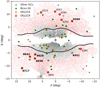 |
Fig. 1. Galactic coordinates of the bulge region, with the black contours as the COBE/DIRBE outline (Jönsson et al. 2017). The small symbols are all RRLs from the OGLE-IV survey (in grey from Soszyński et al. 2014, and in red from Soszyński et al. 2019). The GCs are also shown, with those selected by Bica et al. (2016) as bulge GCs shown in green. The GCs with contours are the ones that contain member RRLs according to Soszyński et al. (2014, 2019). The selected sample of six clusters consists of the objects in common in Bica et al. (2016) and Soszyński et al. (2019), except for NGC 6441. |
From the updated OCVS database, we retrieved a list of RRLs with the I mean magnitude, located inside a circular area around the cluster centre: 15′ for NGC 6266 (to include all the RRLs from Clement et al. 2001) and 10′ for the other clusters. The catalogues were cross-matched in position with the catalogues of Clement et al. (2001, 2017 edition5), which contain the mean V magnitudes. Table 2 gives the number of RRLs retrieved for each cluster in these two catalogues, the number of OGLE-IV RRLs that are actually new, and the number of RRLs in the combined catalogue.
Number of RRLs from Clement et al. (2001) and OGLE-IV catalogues, and retrieved in each stage of the methods referred to in Sect. 4.
3.2. Gaia EDR3: Positions and proper motions
In order to carry out a membership analysis, we accessed the high-precision astrometric and photometric data from the Gaia EDR3. For our samples, the main improvements compared to the previous DR2 were the number of detected sources and smaller PM errors. Following the recommendations of the Gaia collaboration6, the following four corrections were applied to the data: parallax zero-point correction (Lindegren et al. 2021), G-band magnitude and flux correction, flux excess factor correction (Riello et al. 2021), and a recent correction of the PM bias with G magnitude (Cantat-Gaudin & Brandt 2021).
As concerns the catalogue validation, four suggested criteria were tested: G ≤ 19 mag (Fabricius et al. 2021), GRP ≤ 20 mag, |phot_bp_rp_excess_factor| < 5σC* (Riello et al. 2021), and re-normalised unit weight error (ruwe) < 1.4 (Gaia Collaboration 2021b). Riello et al. (2021) show that the filtering in σC* removes sources with inconsistencies between the G, BP, and RP photometry, affecting the completeness of variable and extended sources. In fact, some central RRLs were filtered in these clusters, and we opted not to use this filtering and to loosen the last restriction to ruwe < 2.0 (since ruwe is higher in crowded areas; Lindegren et al. 2021). With these changes, we obtained filtered samples (Nfilt; Table 2) more similar to Gaia DR2.
After transforming the Gaia ICRS coordinates to J2000, we cross-matched the Gaia EDR3 catalogues, appending the PMs and Gaia magnitudes to our combined catalogue. We applied a two-dimensional Gaussian mixture model (GMM) to a group of more central stars against the remaining field stars. The radius limiting this group of central stars was obtained iteratively as the minimum radius that returns a convergence of both cluster and field PMs in right ascension and declination directions. The GMM method assumes the data are clustered in the parameter space following a superposition of Gaussian distributions and it uses the expectation-maximisation algorithm to determine the parameters of each distribution and a correlation matrix (Press et al. 2007). In this case, there are two Gaussian distributions (the cluster distribution with a lower dispersion versus the field stars) in a two-dimensional PM plane. It was applied using using the Python library scikit-learn (Pedregosa et al. 2011).
A membership probability of the RRLs was computed using the equations from Bellini et al. (2009), which consider the measured PMs of each RRL, the cluster and the field, and also their respective uncertainties. Figure 2 shows the coordinates of the RRLs in the field around the six sample GCs, colour-coded with the final membership values. Since the membership was considered when computing the weighted average of the mean magnitudes (Sect. 4.1), no lower cut was applied and all the RRLs were maintained in the catalogues.
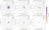 |
Fig. 2. Equatorial coordinates of the RRLs (Nfilt) located inside a radius of 15′ around NGC 6266, and 10′ for the other five GCs. The computed membership is represented by the colour bar, between 0 and 1. The stars from Gaia EDR3, filtered by the catalogue validation (Gaia Collaboration 2021b; Fabricius et al. 2021; Riello et al. 2021) are shown as grey symbols in the background. |
The PM diagrams of the six sample clusters are presented in Fig. 3, showing the centre and dispersion of the two fitted Gaussian distributions, and the groups of central and field stars. The computed PMs in right ascension and declination (μα cos δ and μδ) are given in the first columns of Table 3. The values are very coherent with those from Vasiliev & Baumgardt (2021), which were also derived with Gaia EDR3 data.
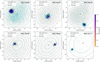 |
Fig. 3. PM diagram of the sample clusters, with the RR Lyrae colour-coded by the membership values. The background stars are divided into those that are more central and those that are further out, shown as cyan and grey points. The two-dimensional Gaussian distributions mark the central cluster and field PMs, along with the dispersions (contour lines mark 0.25 − 2σ in steps of 0.25σ), as derived from the GMM method. The diagrams in the lower panels are zoomed in due to the lower dispersion of the cluster PMs. |
The final RR Lyrae catalogues of the six sample GCs, combining the data from OGLE-IV, Clement et al. (2001), and Gaia EDR3, along with the membership probability values, are provided by us via the VizieR platform. The database can contribute to a wide range of studies by providing a sample of member RRLs for these clusters and removing foreground or background ones.
4. Methods: Distances from OGLE mean magnitudes
In this section, we describe the methods applied to calculate the heliocentric distances: going from computing the average of the mean magnitudes (⟨V⟩ from Clement et al. 2001 catalogues, and ⟨I⟩ from Soszyński et al. 2019), to the determination of the adequate MV − MI − [Fe/H] relations from a Bag of Stellar Tracks and Isochrones7 (BaSTI; Pietrinferni et al. 2021) models, and a discussion on the proper reddening laws to be applied in such a relatively high-reddening regime.
Even more so than the new RRLs detected in Soszyński et al. (2019, see Table 2), the main contribution of the new OGLE-IV catalogues to our analysis are the well-calibrated mean I magnitudes, since this analysis is normally done in the V band. However, from this point on, we proceed with the analysis of both V and I bands, allowing one to compare the results and argue about systematic differences.
4.1. Weighted average of the mean magnitudes
The light curves, I-band amplitudes, and mean magnitudes given in the new OGLE-IV catalogues are a combination of 20 − 200 exposures of 25 s, with a median value of 112 epochs (Soszyński et al. 2019). The data are part of the Galaxy Variability Survey, which are ∼1 mag shallower than the original OGLE photometry. According to Soszyński et al. (2019), the photometric saturation limit is I ∼ 11 mag and the faint limit is I ∼ 19.5 mag. This magnitude range is enough to study the RRLs and HB of several bulge GCs since they populate the CMDs around I ∼ 15 (or V ∼ 16) in this reddening regime.
We calculated an average of these mean magnitudes, which are quite stable around the RRL locus of old GCs. As mentioned before, the averages ⟨V⟩ and ⟨I⟩ are based on the mean V and I magnitudes by Clement et al. (2001) and Soszyński et al. (2019). These averages were calculated with a weight for each RRL, corresponding to its memberships pi and pj:
 (1)
(1)
where the indexes i and j of the two summations go from 1 to NV and NI, respectively.
Moreover, we applied a sigma clipping to iteratively remove the outliers located beyond 2σ from the median magnitude, until a convergence was reached, where σ is the standard deviation. Since the outliers were mostly low-pi RRLs, the central results do not change much, but the final standard error of the weighted mean is reduced by half due to the smaller dispersion of the adopted points. The sigma clipping is crucial because the magnitude of the outliers could be scattered by physical double stars or by other peculiar errors.
The results on the weighted average of mean V and I magnitudes, along with the standard error and the number of stars considered in each case, are also given in Table 3. The number of stars (NV and NI) corresponds to the stars with available mean magnitudes which are present in the filtered Gaia EDR3 catalogues, excluding those with PM errors greater than 0.20 mas yr−1. Figures 4 and 5 show the ⟨V⟩ and ⟨I⟩ versus period plots for the clusters with more than one member RRL with available magnitudes, with the RRLs colour-coded by its membership results.
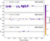 |
Fig. 4. Mean V magnitude (Clement et al. 2001) versus period of pulsation for the RRLs of NGC 6266, NGC 6441, and NGC 6626. The stars are colour-coded by the derived membership, and the empty symbols correspond to stars that were removed using the sigma clipping method (median ± 2σ). The dashed black line represents the weighted average, and the dotted lines give the standard error and the 2σ level. |
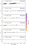 |
Fig. 5. Mean I magnitude (Soszyński et al. 2019) versus period for the six sample clusters. The details are the same as in Fig. 4. |
It is clear from Fig. 2 that the radius alone is not a valid parameter for selecting member RRLs since several central RRLs have a low PM-based membership, and vice versa. Figures 4 and 5 also show that some RRLs with a low membership have apparent magnitudes close to the weighted average, that is they have the same distance as the cluster. Therefore, it is possible that some real RRL members returned low membership values, but it is also expected that the large number of RRLs reduces this bias.
4.2. MV− and MI−[Fe/H] relations from BaSTI α-enhanced models
Several luminosity-metallicity relations are available in the literature with slightly different slopes (e.g., Sandage 1993; Clementini et al. 2003; Gaia Collaboration 2017). The relations between absolute magnitude and metallicity are normally given in the V band (MV − [Fe/H]), whereas in the near- and mid-infrared a period–luminosity or period–luminosity–metallicity relation is obtained (e.g., PMKSZ in Muraveva et al. 2018). Most of them employ nearby field RRLs, possibly Population I stars, younger than our very old, metal-poor, α-enhanced bulge sample.
Large samples of RRLs with accurate trigonometric parallaxes are required to calibrate (period–)luminosity–metallicity relations. Such a large sample was made possible with the recent Gaia mission, containing around 400 MW RRLs. Here, we compare the following two recent works that derived MV − [Fe/H], along with other relations, adopting the Gaia parallaxes: Gaia Collaboration (2017) and Muraveva et al. (2018).
Gaia Collaboration (2017) calibrated MV − [Fe/H] relations based on parallaxes from the Tycho-Gaia Astrometric Solution (TGAS) from Gaia DR1 (Gaia Collaboration 2016a). They applied three different methods to perform this calibration, fixing the slope in 0.214 ± 0.047 mag/dex, as determined in two earlier photometric and spectroscopic studies of RRLs in the Large Magellanic Cloud bar (Clementini et al. 2003; Gratton et al. 2004), returning ![Mathematical equation: $ M_V = 0.214\rm{[Fe/H]} + 0.88^{+0.04} _{-0.06} $](/articles/aa/full_html/2022/01/aa41596-21/aa41596-21-eq2.gif) .
.
On the other hand, Muraveva et al. (2018) derived MV − [Fe/H] by adopting photometric data from Dambis et al. (2013) and parallaxes from Gaia DR2, obtaining MV = (0.34 ± 0.03)·[Fe/H]+(1.17±0.04) for 381 RRLs. This higher slope is closer to those from Sandage (1993) and Feast (1997), but steeper than that from Gaia Collaboration (2017). This difference can be due to the zero-point offset affecting the Gaia DR2 parallaxes (Arenou et al. 2018) and the assumed metallicity values from Dambis et al. (2013). When limiting their study to a smaller sample of 23 RRLs with a metallicity from high-resolution spectroscopy, Muraveva et al. (2018) obtained MV = (0.25±0.05)[Fe/H]+(1.18±0.12), which is much closer to the recent literature.
For the present work, we decided to estimate the distance to the selected clusters by using the theoretical distance scale based on the most updated set of BaSTI stellar models (Hidalgo et al. 2018; Pietrinferni et al. 2021). In more detail, since we were faced with metal-poor, α-enhanced star clusters, we selected the α-enhanced version of the BaSTI library recently provided by Pietrinferni et al. (2021): the predicted magnitudes in the VI Johnson-Cousin bands of zero-age horizontal branch (ZAHB) models located within the RRL instability strip (log Teff = 3.83) were used to derive the dependence of the HB brightness (in these specific photometric passbands) on the metallicity. Since we are interested in comparing the average magnitude of the RRL sample in each cluster with the theoretical predictions, we corrected the ZAHB brightness by applying a calibration from Cassisi & Salaris (1997) in order to properly account for the post-ZAHB evolutionary effects that impact on the RRL luminosity distribution (we refer to Cassisi et al. 2004, for a detailed discussion on this issue).
The GC NGC 6441 as its twin NGC 6388, at odds with its metal content, shows an extended blue HB (Rich et al. 1997), and hosts a peculiar class of RRL characterised by anomalously large pulsation periods, defining the peculiar Oosterhoff class named OoIII (Pritzl et al. 2003). Detailed HB simulations (Busso et al. 2007; Tailo et al. 2017) have shown that the peculiar HB morphology and the pulsational properties of its RRL population can be explained by accounting for the presence of a helium-enhanced stellar population with Y ∼ 0.35 − 0.40. With the RRLs in NGC 6441 being the progeny of this He-enhanced sub-population, they cross the instability strip at a larger luminosity, and hence a longer period, than normal He RRLs. To take this occurrence into account, we adopted He-enhanced BaSTI ZAHB models with Y = 0.35 to estimate the RRL strip luminosity level, which is to be applied for estimating the distance to NGC 6441.
Figure 6 shows the absolute magnitudes MV and MI versus the metallicity of the ZAHB models (black points). The metallicity ranges between −2.20 and +0.06, and the vertical error bars are assumed to be of 0.05. The coefficients of the quadratic function (red curves), better following the points than a linear one, were obtained with a Markov chain Monte Carlo method (using the Python library emcee; Foreman-Mackey et al. 2013), along with the respective uncertainties. The dotted line shows the relationship derived for the He-enhanced ZAHB models (Y = 0.35), adopted for the case of NGC 6441.
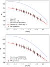 |
Fig. 6. Quadratic fits of the luminosity-metallicity relations MV − [Fe/H] and MV − [Fe/H]. The black points are BaSTI α-enhanced zero-age HB models, corrected by the calibration from Cassisi & Salaris (1997) to account a dispersion of the RRLs due to their evolution. The quadratic functions (red for canonical He, as in Eqs. (2) and (3), and dotted blue for enhanced He) were obtained via the Markov chain Monte Carlo method. |
The second-order polynomial fits for the models with canonical He with the uncertainties on the coefficients are as follows:
![Mathematical equation: $$ \begin{aligned}&M_V = (1.047 \pm 0.028) + (0.456 \pm 0.063)\cdot \mathrm{[Fe/H]} \nonumber \\&\qquad +(0.077\pm 0.030)\cdot \mathrm{[Fe/H]} ^2 \end{aligned} $$](/articles/aa/full_html/2022/01/aa41596-21/aa41596-21-eq3.gif) (2)
(2)
![Mathematical equation: $$ \begin{aligned}&M_I = (0.619 \pm 0.028) + (0.455 \pm 0.063)\cdot \mathrm{[Fe/H]} \nonumber \\&\qquad +(0.075 \pm 0.030)\cdot \mathrm {[Fe/H]}^2 . \end{aligned} $$](/articles/aa/full_html/2022/01/aa41596-21/aa41596-21-eq4.gif) (3)
(3)
The MV − [Fe/H] relations from Gaia Collaboration (2017) and Muraveva et al. (2018) are also presented in the upper panel of Fig. 6. Our derived relations from BaSTI ZAHB models are more consistent with Gaia Collaboration (2017) but they deviate towards fainter magnitudes at higher metallicites. For a metallicity of [Fe/H] = −1.15, which is the average metallicity of our sample and the metallicity of the prototypical RR Lyrae star, the Muraveva et al. (2018) relation would result in a 0.12 smaller (m − M)V, underestimating the final distances.
4.3. Reddening laws and coefficients
For both the V and I filters, subtracting the average of the mean magnitudes and the luminosity–metallicity relation evaluated for the assumed [Fe/H] gives the apparent distance modulus, which in turn provides the final distance with the proper reddening laws and coefficients. Our aim is to obtain the most up-to-date photometric distances in the I band. For this, three main points on the reddening laws have to be examined: (i) the average reddening law, quantified as RV = AV/E(B − V); (ii) the corresponding extinction coefficient for the I filter, represented by AI/E(B − V) or AI/AV; and (iii) the dependence on the effective temperature of the extinction (see, e.g., the discussion in Bedin et al. 2009). The effect of these transformations is increasingly important for higher reddening.
As far as what concerns the first point, the total-to-selective extinction ratio RV is commonly assumed as the constant of correlation between extinction AV and reddening E(B − V), but it is not constant and depends on the intrinsic colour and the amount of reddening (e.g., Blanco 1956; Olson 1975). The RV ratio has been obtained by several authors in the past, from Whitford (1958) and Johnson (1965), and more recently by Schlegel et al. (1998) and Schlafly et al. (2016), based on a large number of stars from the SDSS, 2MASS, and Pan-STARRS surveys. A deep and clear review is given in McCall (2004). While there is a variety of RV values for specific regions of the Galaxy, ranging from 2.8 up to 5.0 (e.g., Cardelli et al. 1989; Fitzpatrick 1999, which used early-type O and B stars), there is a convergence to ∼3.1. This value is very close to the earlier value of 3.0 (Schmidt-Kaler 1961).
Surprisingly, Schlafly et al. (2016) obtained an average RV of 3.32 ± 0.18 from thousands of stars sparse in the Galactic plane (see their Fig. 15). As explained by the authors, this relatively higher value (3.3 vs. 3.1) is justified by the fact that their sample is based on a wide sample of unselected red giant stars with an average temperature of about 4500 K and E(B − V) = 0.65. This corresponds to B − V = 1.0 − 1.1 (K stars).
As discussed in Casagrande & VandenBerg (2014), for a given E(B − V), the RV ratio is almost a linear function of the spectral type since the reddening produces a different effective wavelength for each filter. For MW stars obscured by normal dust, Schmidt-Kaler (1982) related the effective total-to-selective extinction ratio with the reddening with the following equation:  , where (B − V)0 is the intrinsic colour, and
  is the RV ratio for a star of zero-colour in the limit of zero reddening (McCall 2004).
Correcting the Schlafly et al. (2016) value with the Schmidt-Kaler equation to A0 (Vega) type stars, we obtained  , which is coherent with the earlier references within the errors. In our case of V photometry (Clement et al. 2001) for RR Lyrae variables, we adopted an average E(B − V) = 0.5 and (B − V) = 0.35 (A5–F5 spectral type). Adopting the zero-reddening extrapolation of
  for Vega (McCall 2004), we obtained a coefficient of RV = 3.19. However, the fact that the present sample is located close to the Galactic plane and towards the bulge suggests that RV may be lower than 3.1, as discussed in recent works (Nataf et al. 2013; Casagrande & VandenBerg 2014; Saha et al. 2019). By combining optical and NIR data, Pallanca et al. (2021) argue that RV = 2.7 in the direction of the bulge GC NGC 6440 (ℓ = 7.° 73, b = +3.° 80). For our sample GCs (5° < |b|< 10°), we adopted a more conservative value of RV = 3.0.
The second point listed above concerns the wavelength dependence of the interstellar extinction, more specifically in the I band, for which the OGLE data are available. One of the most updated references on BVI extinction relations is Fitzpatrick (1999), who provided the extinction curve for several wavelengths and computed extinction ratios for the Johnson and Strömgren filters. For the I filter, Fitzpatrick (1999) derived a ratio of AI/E(B − V) = 1.57, which is very close to the earlier value of 1.50 from Schultz & Wiemer (1975).
However, Fitzpatrick (1999) derived those relations for very blue stars (Teff = 30 000 K and log g = 4.0), while we used RR Lyrae stars with temperatures just lower than 10 000 K. For this temperature regime, the ratio should be greater than 1.57, resulting in smaller distances for heavily reddened GCs. In following work, McCall (2004) obtained AI/E(B − V) = 1.71 (see their Table 1), under the assumption of RV = 3.07 for Vega at zero-reddening extrapolation.
The sensitivity of this coefficient to the temperature of the stars and to the reddening is not very high and can be obtained using PARSEC (PAdova and TRieste Stellar Evolution Code8; Bressan et al. 2012) isochrones fitted with the reddening law at different AV values. The PARSEC isochrones are not fully reliable to provide the zero point transformations, since they assume RV = 3.1 for G2V stars (this value was derived for a Vega-type star and gives about 3.3 when extrapolated to a G2V star). Scaling the coefficient with PARSEC, for the same values B − V = 0.3 and AV = 1.5, the derived correction from Vega colours is only 0.007, which is much smaller than the analogous AV/E(B − V) correction of 0.12 and is an advantage of adopting the I band instead of V.
In conclusion, assuming the correct E(B − V) is used, the correct coeffient is AI/E(B − V) = 1.703 for the RR Lyrae stars. Applying the correction due to the bulge region in RV from 3.19 to 3.0 (a factor of 0.94 smaller), we obtained a final coefficient ratio of AI/E(B − V) = 1.60.
The last point to be examined is the reddening variations of the coefficients. All the E(B − V) input values from the literature (Sect. 2) have been obtained from SGB F-type stars at the HB level, which corresponds to an intrinsic (B − V) = 0.8 − 0.9. Therefore, the spectra are very different from the Vega and RR Lyrae stars (B − V = 0.3, on average), and they require the temperature-reddening correction. We can estimate this correction by analysing two figures from McCall (2004): first transform B − V into B − I using Fig. 4, and then using their Fig. 8. From this analysis, we obtained a correction factor of 0.85/0.92 or 1/1.07. The literature E(B − V) should be decreased by about 1/1.07 (or increased by a factor 1.07) to get the correct reddening for the RRLs.
Gathering these corrections on the extinction coefficients and reddening, the equations we adopted to obtain the extinctions in the V and I filters are as follows:
![Mathematical equation: $$ \begin{aligned} \ A_V = [E(B-V)\cdot 1.07]\cdot 3.0 \end{aligned} $$](/articles/aa/full_html/2022/01/aa41596-21/aa41596-21-eq9.gif) (4)
(4)
![Mathematical equation: $$ \begin{aligned} \ A_I = [E(B-V) \cdot 1.07] \cdot 1.6. \end{aligned} $$](/articles/aa/full_html/2022/01/aa41596-21/aa41596-21-eq10.gif) (5)
(5)
In the three clusters with available data in VI bands, it is possible to calculate an E(V − I) value for each RRL by subtracting the (V − I)* colour from the apparent magnitudes (Sect. 4.1) from the absolute (MV − MI) colour (Sect. 4.2). The result for each RRL could also account for the differential reddening across the cluster. The colour excess E(V − I) is also defined as AV − AI, and it can be converted to E(B − V) with Eqs. (4) and (5):
![Mathematical equation: $$ \begin{aligned} \ E(V-I) = [E(B-V)\cdot 1.07] \cdot (3.0{-}1.6) \end{aligned} $$](/articles/aa/full_html/2022/01/aa41596-21/aa41596-21-eq11.gif) (6)
(6)
 (7)
(7)
The resulting average E(B − V) values are coherent with the literature ones (Sect. 2), with a small dispersion among the cluster RRLs. Given that the computed reddening did not vary much, becoming irrelevant to detect differential reddening, we opted to just update the input E(B − V) with an average of the computed E(B − V) for these three GCs, and not to use it separately star-by-star. Therefore, we updated the inputs as follows: 0.47 ± 0.05 to 0.50 ± 0.05 for NGC 6266, 0.47 ± 0.05 to 0.44 ± 0.05 for NGC 6441, and 0.43 ± 0.04 to 0.42 ± 0.04 for NGC 6626.
5. Results on the final distances
All the methods and equations described in Sect. 4, along with a complete uncertainty propagation, were applied to obtain the final distances. Table 4 shows the results of the absolute magnitudes, distance moduli, and distances using both I and V bands. For NGC 6638 and NGC 6642, we could not derive the distance with the mean V magnitudes since they are not available in Clement et al. (2001) catalogues.
Results of the absolute magnitudes, distance moduli, and distances obtained from the mean I and V magnitudes and BaSTI ZAHB models.
Despite the study of the mean I magnitudes of the RRLs with the new OGLE-IV data (Soszyński et al. 2019) being our main science case, the calculations with the V magnitudes (Clement et al. 2001) contribute to the argument about the systematics between the different bands. From Table 4, it is clear that the results with ⟨V⟩, instead of being close to the ones with ⟨I⟩, have higher uncertainties, which may be explained by the differential reddening, lower statistics of RRLs, and an inhomogeneity of the compiled data from Clement et al. (2001) as compared to OGLE data.
Figure 7 compares the ratio of our distances derived with the I band (DI) with those from Baumgardt & Vasiliev (2021) and Vasiliev & Baumgardt (2021) listed in Table 4, as a function of DI. The difference between our distances DI and the literature average from Baumgardt & Vasiliev (2021) is less than 5% for the six GCs and within our derived uncertainties. On the other hand, the comparison with Vasiliev & Baumgardt (2021) shows a discrepancy up to 10 − 20% for the three closest clusters (NGC 6626, NGC 6266, and NGC 6717). The uncertainties of ∼10% in Gaia EDR3 parallaxes, the high-reddening region of the bulge, and a possible offset of 0.007 mas in the zero-point correction from Lindegren et al. (2021) may explain this discrepancy.
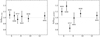 |
Fig. 7. Ratio of the distances derived in this work (DI, Table 4), with the average distances from Baumgardt & Vasiliev (2021, BV21, left panel) and the distances derived from parallaxes from Vasiliev & Baumgardt (2021, VB21, right panel). The vertical error bars correspond to the derived uncertainties, divided by DBV21 or DVB21. The distances from Vasiliev & Baumgardt (2021) are discrepant with ours only for the three closest GCs (10% for NGC 6626, and 20% for NGC 6266 and NGC 6717). |
The two sample clusters with fewer RRLs (NGC 6642 and NGC 6717) provided interesting results. For NGC 6717, the only RR Lyrae, with ⟨B⟩ = 15.75 (Goranskii 1979) or ⟨V⟩ = 15.70 (Ortolani et al. 1999), is exactly the same one that is the only cluster RRL member, and that sets the ⟨I⟩ average around 14.88 (Figs. 3 and 5). The derived DV and DI distances are very close to Oliveira et al. (2020), and to the average from Baumgardt & Vasiliev (2021) which is mainly based on optical models fitting for this cluster. For NGC 6642, the reddening values are divergent. It seems that the E(B − V) = 0.6 from Valenti et al. (2007) is overestimated, and would result in a lower distance. A new analysis with deep photometry and isochrone fitting would be an important validation test for this cluster.
6. Conclusions
The sample of six globular clusters was selected for having newly identified lists of RR Lyrae from the OGLE survey. It is interesting to note that Pérez-Villegas et al. (2020) assigned four of these clusters to a bulge population, and two of them (NGC 6441 and NGC 6638) as belonging to a thick disk population. Massari et al. (2019) assigned all of them, except NGC 6441, as belonging to the main bulge, and NGC 6441 would be in an unassociated low-energy category.
The distances derived are compatible with those derived by Baumgardt et al. (2019) and the average distances from Baumgardt & Vasiliev (2021), considering the uncertainties. When comparing them to the distances derived from Gaia EDR3 parallaxes in Vasiliev & Baumgardt (2021), a discrepancy of 10 − 20% is observed for NGC 6266, NGC 6626, and NGC 6717, which can be explained by some limitations, possibly an offset in the zero-point correction from Lindegren et al. (2021). Since our method is based on a bona fide sample of member RRLs, recent BaSTI models, correct relations for reddening, and a robust method, it was already expected that our distances would be very close to the average distances from Baumgardt & Vasiliev (2021), based mainly on photometric derivations.
A wider sample will be adopted in a future work in order to revise the bulge cluster distance, related to the Sun-Galactic centre distance (Bland-Hawthorn & Gerhard 2016). In fact, the uncertainties of 5 − 8% obtained in this method show it is a solid basis for new distance measurements, as a complement to the recent geometric methods. The final catalogues of RRLs with data from Clement et al. (2001), OGLE-IV (Soszyński et al. 2019) and Gaia EDR3 (Gaia Collaboration 2021a), and the computed membership values are provided in VizieR.
Available at: http://basti-iac.oa-abruzzo.inaf.it.
Acknowledgments
R.A.P.O. and S.O.S. acknowledge the FAPESP PhD fellowships nos. 2018/22181-0 and 2018/22044-3 respectively. B.B., L.O.K. and E.B. acknowledge partial financial support from FAPESP, CNPq, and CAPES – Finance Code 001. S.O. acknowledges partial support by the Università degli Studi di Padova Progetto di Ateneo BIRD178590. S.C. acknowledges support from Progetto Mainstream INAF (PI: S. Cassisi), from INFN (Iniziativa specifica TAsP), and from PLATO ASI-INAF agreement n.2015-019-R.1-2018. A.P.V. acknowledges the DGAPA-PAPIIT grant IG100319. This work has made use of data from the European Space Agency (ESA) mission Gaia (https://www.cosmos.esa.int/gaia), processed by the Gaia Data Processing and Analysis Consortium (DPAC, https://www.cosmos.esa.int/web/gaia/dpac/consortium). Funding for the DPAC has been provided by national institutions, in particular the institutions participating in the Gaia Multilateral Agreement. We thank an anonymous referee for the remarks that improved this paper.
References
- Alonso-García, J., Mateo, M., Sen, B., Banerjee, M., & von Braun, K. 2011, AJ, 141, 146 [CrossRef] [Google Scholar]
- Alonso-García, J., Mateo, M., Sen, B., et al. 2012, AJ, 143, 70 [Google Scholar]
- Alonso-García, J., Smith, L. C., Catelan, M., et al. 2021, A&A, 651, A47 [NASA ADS] [CrossRef] [EDP Sciences] [Google Scholar]
- Arenou, F., Luri, X., Babusiaux, C., et al. 2018, A&A, 616, A17 [NASA ADS] [CrossRef] [EDP Sciences] [Google Scholar]
- Bailey, S. I. 1902, Ann. Harvard College Obs., 38, 1 [Google Scholar]
- Balbinot, E., Santiago, B. X., Bica, E., & Bonatto, C. 2009, MNRAS, 396, 1596 [NASA ADS] [CrossRef] [Google Scholar]
- Barbuy, B., Bica, E., Ortolani, S., & Bonatto, C. 2006, A&A, 449, 1019 [NASA ADS] [CrossRef] [EDP Sciences] [Google Scholar]
- Barbuy, B., Chiappini, C., & Gerhard, O. 2018, ARA&A, 56, 223 [Google Scholar]
- Baumgardt, H., & Hilker, M. 2018, MNRAS, 478, 1520 [Google Scholar]
- Baumgardt, H., & Vasiliev, E. 2021, MNRAS, 505, 5957 [NASA ADS] [CrossRef] [Google Scholar]
- Baumgardt, H., Hilker, M., Sollima, A., & Bellini, A. 2019, MNRAS, 482, 5138 [Google Scholar]
- Beccari, G., Ferraro, F. R., Possenti, A., et al. 2006, AJ, 131, 2551 [NASA ADS] [CrossRef] [Google Scholar]
- Bedin, L. R., Salaris, M., Piotto, G., et al. 2009, ApJ, 697, 965 [NASA ADS] [CrossRef] [Google Scholar]
- Bellini, A., Piotto, G., Bedin, L. R., et al. 2009, A&A, 493, 959 [NASA ADS] [CrossRef] [EDP Sciences] [Google Scholar]
- Bica, E., Bonatto, C., Barbuy, B., & Ortolani, S. 2006, A&A, 450, 105 [NASA ADS] [CrossRef] [EDP Sciences] [Google Scholar]
- Bica, E., Ortolani, S., & Barbuy, B. 2016, PASA, 33, e028 [Google Scholar]
- Blanco, V. M. 1956, ApJ, 123, 64 [NASA ADS] [CrossRef] [Google Scholar]
- Bland-Hawthorn, J., & Gerhard, O. 2016, ARA&A, 54, 529 [Google Scholar]
- Bressan, A., Marigo, P., Girardi, L., et al. 2012, MNRAS, 427, 127 [NASA ADS] [CrossRef] [Google Scholar]
- Brocato, E., Buonanno, R., Malakhova, Y., & Piersimoni, A. M. 1996, A&A, 311, 778 [NASA ADS] [Google Scholar]
- Busso, G., Cassisi, S., Piotto, G., et al. 2007, A&A, 474, 105 [NASA ADS] [CrossRef] [EDP Sciences] [Google Scholar]
- Cadelano, M., Ransom, S. M., Freire, P. C. C., et al. 2018, ApJ, 855, 125 [Google Scholar]
- Cantat-Gaudin, T., & Brandt, T. D. 2021, A&A, 649, A124 [NASA ADS] [CrossRef] [EDP Sciences] [Google Scholar]
- Cardelli, J. A., Clayton, G. C., & Mathis, J. S. 1989, ApJ, 345, 245 [Google Scholar]
- Carretta, E., Bragaglia, A., Gratton, R., D’Orazi, V., & Lucatello, S. 2009, A&A, 508, 695 [NASA ADS] [CrossRef] [EDP Sciences] [Google Scholar]
- Casagrande, L., & VandenBerg, D. A. 2014, MNRAS, 444, 392 [Google Scholar]
- Cassisi, S., & Salaris, M. 1997, MNRAS, 285, 593 [NASA ADS] [Google Scholar]
- Cassisi, S., Castellani, M., Caputo, F., & Castellani, V. 2004, A&A, 426, 641 [NASA ADS] [CrossRef] [EDP Sciences] [Google Scholar]
- Clement, C. M., Muzzin, A., Dufton, Q., et al. 2001, AJ, 122, 2587 [NASA ADS] [CrossRef] [Google Scholar]
- Clementini, G., Gratton, R., Bragaglia, A., et al. 2003, AJ, 125, 1309 [CrossRef] [Google Scholar]
- Contreras, R., Catelan, M., Smith, H. A., et al. 2010, AJ, 140, 1766 [NASA ADS] [CrossRef] [Google Scholar]
- Dall’Ora, M., Stetson, P. B., Bono, G., et al. 2008, Mem. Soc. Astron. It., 79, 355 [Google Scholar]
- Dambis, A. K., Berdnikov, L. N., Kniazev, A. Y., et al. 2013, MNRAS, 435, 3206 [Google Scholar]
- Davidge, T. J., Cote, P., & Harris, W. E. 1996, ApJ, 468, 641 [Google Scholar]
- Dotter, A., Sarajedini, A., Anderson, J., et al. 2010, ApJ, 708, 698 [Google Scholar]
- Fabricius, C., Luri, X., Arenou, F., et al. 2021, A&A, 649, A5 [NASA ADS] [CrossRef] [EDP Sciences] [Google Scholar]
- Feast, M. W. 1997, MNRAS, 284, 761 [NASA ADS] [CrossRef] [Google Scholar]
- Ferraro, F. R., Messineo, M., Fusi Pecci, F., et al. 1999, AJ, 118, 1738 [NASA ADS] [CrossRef] [Google Scholar]
- Fitzpatrick, E. L. 1999, PASP, 111, 63 [Google Scholar]
- Foreman-Mackey, D., Hogg, D. W., Lang, D., & Goodman, J. 2013, PASP, 125, 306 [Google Scholar]
- Gaia Collaboration (Prusti, T., et al.) 2016a, A&A, 595, A1 [NASA ADS] [CrossRef] [EDP Sciences] [Google Scholar]
- Gaia Collaboration (Brown, A. G. A., et al.) 2016b, A&A, 595, A2 [NASA ADS] [CrossRef] [EDP Sciences] [Google Scholar]
- Gaia Collaboration (Clementini, G., et al.) 2017, A&A, 605, A79 [NASA ADS] [CrossRef] [EDP Sciences] [Google Scholar]
- Gaia Collaboration (Brown, A. G. A., et al.) 2018, A&A, 616, A1 [NASA ADS] [CrossRef] [EDP Sciences] [Google Scholar]
- Gaia Collaboration (Brown, A. G. A., et al.) 2021a, A&A, 649, A1 [NASA ADS] [CrossRef] [EDP Sciences] [Google Scholar]
- Gaia Collaboration (Antoja, T., et al.) 2021b, A&A, 649, A8 [EDP Sciences] [Google Scholar]
- Goranskii, V. P. 1979, Sov. Astron., 23, 284 [Google Scholar]
- Gratton, R. G., Bragaglia, A., Clementini, G., et al. 2004, A&A, 421, 937 [NASA ADS] [CrossRef] [EDP Sciences] [Google Scholar]
- Harris, W. E. 1996, AJ, 112, 1487 [Google Scholar]
- Heinke, C. O., Wijnands, R., Cohn, H. N., et al. 2006, ApJ, 651, 1098 [NASA ADS] [CrossRef] [Google Scholar]
- Hidalgo, S. L., Pietrinferni, A., Cassisi, S., et al. 2018, ApJ, 856, 125 [Google Scholar]
- Johnson, H. L. 1965, ApJ, 141, 923 [NASA ADS] [CrossRef] [Google Scholar]
- Jönsson, H., Ryde, N., Schultheis, M., & Zoccali, M. 2017, A&A, 598, A101 [NASA ADS] [CrossRef] [EDP Sciences] [Google Scholar]
- Kerber, L. O., Nardiello, D., Ortolani, S., et al. 2018, ApJ, 853, 15 [Google Scholar]
- Kerber, L. O., Libralato, M., Souza, S. O., et al. 2019, MNRAS, 484, 5530 [Google Scholar]
- Lapenna, E., Mucciarelli, A., Ferraro, F. R., et al. 2015, ApJ, 813, 97 [CrossRef] [Google Scholar]
- Lindegren, L., Bastian, U., Biermann, M., et al. 2021, A&A, 649, A4 [EDP Sciences] [Google Scholar]
- Massari, D., Koppelman, H. H., & Helmi, A. 2019, A&A, 630, L4 [NASA ADS] [CrossRef] [EDP Sciences] [Google Scholar]
- McCall, M. L. 2004, AJ, 128, 2144 [Google Scholar]
- McNamara, B. J., & McKeever, J. 2011, AJ, 142, 163 [CrossRef] [Google Scholar]
- Muhie, T. D., Dambis, A. K., Berdnikov, L. N., Kniazev, A. Y., & Grebel, E. K. 2021, MNRAS, 502, 4074 [NASA ADS] [CrossRef] [Google Scholar]
- Muraveva, T., Delgado, H. E., Clementini, G., Sarro, L. M., & Garofalo, A. 2018, MNRAS, 481, 1195 [Google Scholar]
- Nataf, D. M., Gould, A., Fouqué, P., et al. 2013, ApJ, 769, 88 [Google Scholar]
- Oliveira, R. A. P., Souza, S. O., Kerber, L. O., et al. 2020, ApJ, 891, 37 [Google Scholar]
- Olson, B. I. 1975, PASP, 87, 349 [NASA ADS] [CrossRef] [Google Scholar]
- Origlia, L., Valenti, E., & Rich, R. M. 2008, MNRAS, 388, 1419 [NASA ADS] [Google Scholar]
- Ortolani, S., Barbuy, B., & Bica, E. 1999, A&AS, 136, 237 [NASA ADS] [CrossRef] [EDP Sciences] [Google Scholar]
- Ortolani, S., Barbuy, B., Bica, E., Zoccali, M., & Renzini, A. 2007, A&A, 470, 1043 [NASA ADS] [CrossRef] [EDP Sciences] [Google Scholar]
- Ortolani, S., Held, E. V., Nardiello, D., et al. 2019, A&A, 627, A145 [NASA ADS] [CrossRef] [EDP Sciences] [Google Scholar]
- Pallanca, C., Lanzoni, B., Ferraro, F. R., et al. 2021, ApJ, 913, 137 [NASA ADS] [CrossRef] [Google Scholar]
- Pedregosa, F., Varoquaux, G., Gramfort, A., et al. 2011, J. Mach Learn. Res., 12, 2825 [Google Scholar]
- Pérez-Villegas, A., Barbuy, B., Kerber, L. O., et al. 2020, MNRAS, 491, 3251 [Google Scholar]
- Pietrinferni, A., Hidalgo, S., Cassisi, S., et al. 2021, ApJ, 908, 102 [NASA ADS] [CrossRef] [Google Scholar]
- Piotto, G., King, I. R., Djorgovski, S. G., et al. 2002, A&A, 391, 945 [NASA ADS] [CrossRef] [EDP Sciences] [Google Scholar]
- Press, W. H., Teukolsky, S. A., Vetterling, W. T., & Flannery, B. P. 2007, Numerical Recipes 3rd Edition: The Art of Scientific Computing, 3rd edn. (USA: Cambridge University Press) [Google Scholar]
- Pritzl, B. J., Smith, H. A., Catelan, M., & Sweigart, A. V. 2001, AJ, 122, 2600 [Google Scholar]
- Pritzl, B. J., Smith, H. A., Stetson, P. B., et al. 2003, AJ, 126, 1381 [Google Scholar]
- Ransom, S. M., Hessels, J. W. T., Stairs, I. H., et al. 2005, Science, 307, 892 [NASA ADS] [CrossRef] [PubMed] [Google Scholar]
- Reed, B. C., Hesser, J. E., & Shawl, S. J. 1988, PASP, 100, 545 [Google Scholar]
- Rich, R. M., Sosin, C., Djorgovski, S. G., et al. 1997, ApJ, 484, L25 [NASA ADS] [CrossRef] [Google Scholar]
- Riello, M., De Angeli, F., Evans, D. W., et al. 2021, A&A, 649, A3 [NASA ADS] [CrossRef] [EDP Sciences] [Google Scholar]
- Saha, A., Vivas, A. K., Olszewski, E. W., et al. 2019, ApJ, 874, 30 [NASA ADS] [CrossRef] [Google Scholar]
- Sandage, A. 1993, AJ, 106, 703 [NASA ADS] [CrossRef] [Google Scholar]
- Schlafly, E. F., Meisner, A. M., Stutz, A. M., et al. 2016, ApJ, 821, 78 [NASA ADS] [CrossRef] [Google Scholar]
- Schlegel, D. J., Finkbeiner, D. P., & Davis, M. 1998, ApJ, 500, 525 [Google Scholar]
- Schmidt-Kaler, T. 1961, Astron. Nachr., 286, 113 [NASA ADS] [CrossRef] [Google Scholar]
- Schmidt-Kaler, T. 1982, in Landolt-Börnstein, Numerical data and Functional Relationships in Science and Technology, New Series, eds. K. Schaifers, & H. H. Voigt (Berlin: Springer), 2b, 451 [Google Scholar]
- Schultz, G. V., & Wiemer, W. 1975, A&A, 43, 133 [NASA ADS] [Google Scholar]
- Soszyński, I., Udalski, A., Szymański, M. K., et al. 2014, Acta Astron., 64, 177 [NASA ADS] [Google Scholar]
- Soszyński, I., Udalski, A., Wrona, M., et al. 2019, Acta Astron., 69, 321 [Google Scholar]
- Souza, S. O., Kerber, L. O., Barbuy, B., et al. 2020, ApJ, 890, 38 [Google Scholar]
- Tailo, M., D’Antona, F., Milone, A. P., et al. 2017, MNRAS, 465, 1046 [Google Scholar]
- Testa, V., Corsi, C. E., Andreuzzi, G., et al. 2001, AJ, 121, 916 [Google Scholar]
- Valenti, E., Origlia, L., & Ferraro, F. R. 2005, MNRAS, 361, 272 [NASA ADS] [CrossRef] [Google Scholar]
- Valenti, E., Ferraro, F. R., & Origlia, L. 2007, AJ, 133, 1287 [Google Scholar]
- van Agt, S. L. T. J., & Oosterhoff, P. T. 1959, Annalen van de Sterrewacht te Leiden, 21, 253 [NASA ADS] [Google Scholar]
- VandenBerg, D. A., Brogaard, K., Leaman, R., & Casagrande, L. 2013, ApJ, 775, 134 [Google Scholar]
- Vasiliev, E., & Baumgardt, H. 2021, MNRAS, 505, 5978 [NASA ADS] [CrossRef] [Google Scholar]
- Villanova, S., Moni Bidin, C., Mauro, F., Munoz, C., & Monaco, L. 2017, MNRAS, 464, 2730 [Google Scholar]
- Watkins, L. L., van der Marel, R. P., Bellini, A., & Anderson, J. 2015, ApJ, 803, 29 [Google Scholar]
- Webbink, R. F. 1985, in Dynamics of Star Clusters, eds. J. Goodman, & P. Hut, IAU Symp., 113, 541 [Google Scholar]
- Whitford, A. E. 1958, AJ, 63, 201 [NASA ADS] [CrossRef] [Google Scholar]
- Zinn, R. 1985, ApJ, 293, 424 [Google Scholar]
All Tables
Relevant parameters from the literature and input values of metallicity and reddening adopted in this work.
Number of RRLs from Clement et al. (2001) and OGLE-IV catalogues, and retrieved in each stage of the methods referred to in Sect. 4.
Results of the absolute magnitudes, distance moduli, and distances obtained from the mean I and V magnitudes and BaSTI ZAHB models.
All Figures
|
Fig. 1. Galactic coordinates of the bulge region, with the black contours as the COBE/DIRBE outline (Jönsson et al. 2017). The small symbols are all RRLs from the OGLE-IV survey (in grey from Soszyński et al. 2014, and in red from Soszyński et al. 2019). The GCs are also shown, with those selected by Bica et al. (2016) as bulge GCs shown in green. The GCs with contours are the ones that contain member RRLs according to Soszyński et al. (2014, 2019). The selected sample of six clusters consists of the objects in common in Bica et al. (2016) and Soszyński et al. (2019), except for NGC 6441. |
| In the text | |
|
Fig. 2. Equatorial coordinates of the RRLs (Nfilt) located inside a radius of 15′ around NGC 6266, and 10′ for the other five GCs. The computed membership is represented by the colour bar, between 0 and 1. The stars from Gaia EDR3, filtered by the catalogue validation (Gaia Collaboration 2021b; Fabricius et al. 2021; Riello et al. 2021) are shown as grey symbols in the background. |
| In the text | |
|
Fig. 3. PM diagram of the sample clusters, with the RR Lyrae colour-coded by the membership values. The background stars are divided into those that are more central and those that are further out, shown as cyan and grey points. The two-dimensional Gaussian distributions mark the central cluster and field PMs, along with the dispersions (contour lines mark 0.25 − 2σ in steps of 0.25σ), as derived from the GMM method. The diagrams in the lower panels are zoomed in due to the lower dispersion of the cluster PMs. |
| In the text | |
|
Fig. 4. Mean V magnitude (Clement et al. 2001) versus period of pulsation for the RRLs of NGC 6266, NGC 6441, and NGC 6626. The stars are colour-coded by the derived membership, and the empty symbols correspond to stars that were removed using the sigma clipping method (median ± 2σ). The dashed black line represents the weighted average, and the dotted lines give the standard error and the 2σ level. |
| In the text | |
|
Fig. 5. Mean I magnitude (Soszyński et al. 2019) versus period for the six sample clusters. The details are the same as in Fig. 4. |
| In the text | |
|
Fig. 6. Quadratic fits of the luminosity-metallicity relations MV − [Fe/H] and MV − [Fe/H]. The black points are BaSTI α-enhanced zero-age HB models, corrected by the calibration from Cassisi & Salaris (1997) to account a dispersion of the RRLs due to their evolution. The quadratic functions (red for canonical He, as in Eqs. (2) and (3), and dotted blue for enhanced He) were obtained via the Markov chain Monte Carlo method. |
| In the text | |
|
Fig. 7. Ratio of the distances derived in this work (DI, Table 4), with the average distances from Baumgardt & Vasiliev (2021, BV21, left panel) and the distances derived from parallaxes from Vasiliev & Baumgardt (2021, VB21, right panel). The vertical error bars correspond to the derived uncertainties, divided by DBV21 or DVB21. The distances from Vasiliev & Baumgardt (2021) are discrepant with ours only for the three closest GCs (10% for NGC 6626, and 20% for NGC 6266 and NGC 6717). |
| In the text | |
Current usage metrics show cumulative count of Article Views (full-text article views including HTML views, PDF and ePub downloads, according to the available data) and Abstracts Views on Vision4Press platform.
Data correspond to usage on the plateform after 2015. The current usage metrics is available 48-96 hours after online publication and is updated daily on week days.
Initial download of the metrics may take a while.