© The Authors 2024

1. Introduction

The formation of the first sources of radiation at the end of the Universe’s Dark Age is one of the landmark events in Cosmic history. During the first billion years, radiation from the first stars, galaxies, quasars (QSOs), and high-mass X-ray binaries (HMXBs) permanently changed the ionization and thermal state of the Universe. It is expected that radiation from early X-ray sources such as HMXBs and mini-QSOs changed the thermal state of the cold intergalactic medium (IGM) much before the IGM became highly ionized (see, e.g., Pritchard & Furlanetto 2007; Thomas & Zaroubi 2011; Mesinger et al. 2011; Islam et al. 2019; Ross et al. 2019; Eide et al. 2020). The onset of the first sources that changed the IGM’s thermal state is known as the Cosmic Dawn (CD). The subsequent period when the IGM’s atomic neutral hydrogen (H I) became ionized is known as the Epoch of Reionization (EoR). A few indirect probes such as the observations of Gunn-Peterson optical depth in z ≳ 6 QSO spectra and Thomson scattering optical depth of the cosmic microwave background (CMB) photons provide us with useful information about the rough timing and duration of the EoR (see, e.g., Fan et al. 2006; McGreer et al. 2015; Bañados et al. 2018; Planck Collaboration VI 2020; Mitra et al. 2015). However, many details about these epochs, such as the exact timing, properties of the sources and their evolution, feedback mechanisms, and morphology of the ionized and heated regions, are still unknown.

Observations of the redshifted 21 cm radiation produced by H I in the IGM can provide us with information related to the timing, the morphology of the ionized and heated regions, and properties of the ionizing and heating sources (see, e.g., Pritchard & Loeb 2012; Zaroubi 2013; Shaw et al. 2023a; Ghara et al. 2024, for reviews). Many of the world’s large radio observation facilities have aimed for measuring the brightness temperature of this redshifted H I 21 cm radiation (hereafter 21 cm signal) from the CD and EoR. Radio observations using a single antenna, such as EDGES2 (Bowman et al. 2018), SARAS2 (Singh et al. 2017), REACH (de Lera Acedo et al. 2022), and LEDA (Price et al. 2018), aim to measure the redshift evolution of the sky-averaged 21 cm signal. However, observing the morphological distribution of the 21 cm signal in the sky is expected to tell us more about these epochs. Radio interferometers, such as the Low-Frequency Array (LOFAR)¹ (van Haarlem et al. 2013; Patil et al. 2017), the New Extension in Nançay Upgrading LOFAR (NenuFAR)² (Munshi et al. 2024), the Amsterdam ASTRON Radio Transients Facility And Analysis Center (AARTFAAC) (Gehlot et al. 2022), the Precision Array for Probing the Epoch of Reionization (PAPER)³ (Parsons et al. 2014; Kolopanis et al. 2019), the Murchison Widefield Array (MWA)⁴ (e.g. Tingay et al. 2013; Wayth et al. 2018), and the Hydrogen Epoch of Reionization Array (HERA)⁵ (DeBoer et al. 2017), have been commissioned to measure the spatial fluctuations in the H I 21 cm signal at different stages of the CD and EoR.

Due to limited sensitivity, the radio interferometer-based observations aim to detect this signal in terms of the statistical quantities such as the spherically averaged power spectrum (${\mathrm{\Delta }}_{\delta T_{\text{b}}}^2(k,z)$) of the differential brightness temperature (δT_b) of the H I signal at different redshifts (z) and wave-numbers (k). The upcoming Square Kilometre Array (SKA)⁶ will be more sensitive and will also produce tomographic images of the CD and EoR 21 cm signal (Mellema et al. 2015; Ghara et al. 2017).

Observing the 21 cm signal from CD and EoR is very challenging and it has remained undetected by the radio observations to date. The measured H I signal is severely contaminated by the galactic and extra-galactic foregrounds. While the foregrounds are more substantial than the expected CD and EoR H I signal by several orders of magnitude (see, e.g., Ghosh et al. 2012), their smooth frequency dependence allows them to be either subtracted (Harker et al. 2009; Bonaldi & Brown 2015; Chapman et al. 2016; Mertens et al. 2018; Hothi et al. 2021), avoided (Datta et al. 2010; Liu et al. 2014) or suppressed (Datta et al. 2007; Ghara et al. 2016). These observations also face severe challenges at the calibration step of the data analysis process. Nevertheless, recent improvements in the calibration methods (see, e.g., Kern et al. 2019, 2020; Mevius et al. 2022; Gan et al. 2022, 2023), and the mitigation of the foregrounds (e.g., Mertens et al. 2018; Liu et al. 2014) made it possible to obtain noise dominated upper limits of ${\mathrm{\Delta }}_{\delta T_{\text{b}}}^2(k,z)$. For example, ${\mathrm{\Delta }}_{\delta T_{\mathrm{b}}}^2(k=0.14h{\mathrm{Mpc}}^{-1},z=6.5)\approx {(43)}^2{\mathrm{mK}}^2$, ${\mathrm{\Delta }}_{\delta T_{\mathrm{b}}}^2(k=0.075h{\mathrm{Mpc}}^{-1},z=9.1)\approx {(73)}^2{\mathrm{mK}}^2$, and ${\mathrm{\Delta }}_{\delta T_{\mathrm{b}}}^2(k=0.34h{\mathrm{Mpc}}^{-1},z=7.9)\approx {(21.4)}^2{\mathrm{mK}}^2$ are the best upper limits obtained from MWA (Trott et al. 2020), LOFAR (Mertens et al. 2020), and HERA (Abdurashidova et al. 2023) EoR observations, respectively.

These recent upper limits have started to rule out CD and EoR scenarios including those which do not require either an unconventional cooling mechanism or the presence of a strong radio background in addition to the CMB (e.g., Ghara et al. 2020; Greig et al. 2021; Mondal et al. 2020; Abdurashidova et al. 2022a). For example, the recent HERA EoR observation results as reported in Abdurashidova et al. (2022a,b) show that the IGM temperature must be higher than the adiabatic cooling threshold by redshift 8, while the soft band X-ray luminosity per star formation rate of the first galaxies are constrained (1σ level) to [10^40.2 − 10^41.9] erg s⁻¹/(M_⊙ yr⁻¹). In addition, the recent results from the global H I 21 cm signal observations, such as SARAS and EDGES, have also started ruling out EoR and CD scenarios and putting constraints on the properties of the early sources, models of dark matter, and level of radio backgrounds (e.g., Barkana 2018; Fialkov et al. 2018; Muñoz & Loeb 2018; Nebrin et al. 2019; Chatterjee et al. 2019, 2020; Ghara & Mellema 2020; Ghara et al. 2022; Bera et al. 2023).

These previous studies have put constraints mainly on the astrophysical source properties using either Bayesian inference techniques (e.g., Park et al. 2019; Cohen et al. 2020) or Fisher matrices (e.g., Ewall-Wice et al. 2016; Shaw et al. 2020). The main reason behind this is the fact that 21 cm signal simulation codes take the source parameters as input. However, it should be realized that the 21 cm signal measurements do not probe the astrophysical sources directly. In addition, the inference on the properties of the astrophysical sources is limited by the ambiguity of the source model used in the inference framework. The observed 21 cm signal, on the other hand, directly probes the ionization and the thermal states of the IGM. Therefore, we emphatically aim to constrain the IGM properties rather than the astrophysical source parameters.

Previously, Mirocha et al. (2013) considered the features of the redshift evolution of the sky-averaged brightness temperature curves within a simplified global H I signal framework which does not invoke any astrophysical sources and attempted to constrain physical properties of the IGM in terms of Lyα background, overall heat deposition, mean ionization fraction, and their time derivatives. In the context of 21 cm signal power spectrum, studies such as Ghara et al. (2020, 2021) used the recently obtained upper limits from LOFAR (Mertens et al. 2020) and MWA (Trott et al. 2020) to constrain the properties of the IGM at different stages of the EoR. These studies use the outputs from GRIZZLY (Ghara et al. 2015a) simulations and characterize the IGM in terms of quantities such as the sky-averaged ionization fraction, average gas temperature, sky-averaged brightness temperature, the volume fraction of the “heated regions” in the IGM with its brightness temperature T_b larger than the background CMB temperature T_γ, and the characteristic size of these heated regions. For example, using the recent upper limits from LOFAR (Mertens et al. 2020), Ghara et al. (2020) ruled out reionization scenarios at redshift 9.1 where heating of the gas is negligible and the IGM is characterized by ionized fraction ≳0.13, a distribution of the ionized regions with a characteristic size ≳8 h⁻¹ Mpc, and a full width at half-maximum ≳16 h⁻¹ Mpc. In an alternative approach, Shimabukuro et al. (2022) used artificial neural networks to build a framework that estimates the size distribution of the ionized regions using the EoR 21 cm power spectrum.

Our previous studies such as Ghara et al. (2020, 2021), which aim at constraining the properties of the CD and EoR IGM parameters, use source-parameter dependent GRIZZLY simulations. The inputs of their framework are a set of source parameters, such as the ionization efficiency, the minimum mass of dark matter halos that host UV emitting sources, the X-ray emission efficiency, and the minimum mass of dark matter halos that host X-ray emitting sources. The framework provides a set of derived IGM parameters in addition to the 21 cm signal observable. It is not straightforward to build a mathematical framework that directly connects the complex morphology of the IGM to the 21 cm signal observable by skipping the source-parameter dependence. Recently, Mirocha et al. (2022) have attempted to build such a galaxy-free phenomenological model for the EoR 21 cm signal power spectra. The model assumes uniform T_S, spherical ionized bubbles and a binary ionization field. While the model efficiently predicts the 21 cm signal power spectrum for volume average neutral fraction ${\overline{x}}_{\mathrm{HI}}\gtrsim 0.8$, the prediction accuracy rapidly drops for reionization stages with ${\overline{x}}_{\mathrm{HI}}\lesssim 0.8$ which shows the complexity level of the problem.

Unlike our aforementioned IGM inference framework, the main goal of this work is to develop a source parameter-free phenomenological model of EoR 21 cm signal power spectra in terms of quantities related to the IGM. We keep our model simple by ignoring the effect of spin-temperature fluctuations and targeting the IGM only during the EoR. The amplitude and the shape of ${\mathrm{\Delta }}_{\delta T_{\text{b}}}^2(k,z)$ as a function of k during different stages of the EoR depend on the ionization fraction and the complex morphology of the ionized regions at that period. The aim here is to use the multi-redshift measurements of the EoR 21 cm signal power spectra to constrain the IGM properties during the EoR.

This paper is structured as follows. In Sect. 2, we describe the basic methodology of our framework. We present our results in Sect. 3, before concluding in Sect. 4. The cosmological parameters used throughout this study are the same as the N-body simulations employed here (i.e., Ω_m = 0.27, Ω_Λ = 0.73, Ω_B = 0.044, h = 0.7 (Wilkinson Microwave Anisotropy Probe (WMAP); Hinshaw et al. 2013).

2. Framework

2.1. The EoR 21 cm signal

The differential brightness temperature (δT_b) of the 21 cm signal from a region at angular position x and redshift z can be expressed as (see, e.g., Madau et al. 1997; Furlanetto et al. 2006),

$$\begin{array}{cc}\hfill \delta T_{\mathrm{b}}(\mathit{x},z)=& 27x_{\mathrm{HI}}(\mathit{x},z)[1+{\delta }_{\mathrm{B}}(\mathit{x},z)]\left(\frac{{\mathrm{\Omega }}_{\mathrm{B}}{h}^2}{0.023}\right)\hfill \\ \hfill & \times {\left(\frac{0.15}{{\mathrm{\Omega }}_{\mathrm{m}}{h}^2}\frac{1+z}{10}\right)}^{1/2}[1-\frac{T_{\gamma }(z)}{T_{\mathrm{S}}(\mathit{x},z)}]\mathrm{mK}.\hfill \end{array}$$(1)

Here T_S, x_HI, and δ_B are respectively the spin temperature of H I, the neutral hydrogen fraction, and the baryonic density contrast of the region located at (x, z). The quantity T_γ is the radio background temperature at 21 cm wavelength for redshift z. In this study, we assume a high spin temperature limit, i.e., T_S ≫ T_γ. This is expected to be the case in the presence of efficient X-ray heating.

Here, we use the GRIZZLY code (Ghara et al. 2015a,b) to generate brightness temperature maps during the EoR. The inputs for this code are the uniformly gridded dark-matter density and velocity field cubes and the corresponding dark-matter halo list. The GRIZZLY simulations considered in this study use the dark-matter fields and the corresponding halo lists within comoving cubes of side 500 h⁻¹ Mpc, produced from the PRACE⁷ project PRACE4LOFAR N-body simulations (see e.g., Giri et al. 2019; Kamran et al. 2021, for the details of the simulation). The simulation assumes that all dark-matter halos with masses larger than M_min contribute to reionization. The stellar mass M_⋆ inside a halo of mass M_halo is assumed to be $M_{\star }\propto M_{\text{halo}}^{{\alpha }_s}$. We choose the ionization efficiency (ζ) so that the reionization process ends roughly at z ∼ 6.5⁸. The reionization models considered in this study are inside-out in nature where the very dense regions around the sources get ionized first. We refer to Ghara et al. (2015a); Ghara et al. (2020) for the details of the method and the source parameters. Our fiducial GRIZZLY model, as shown in Fig. 1, corresponds to a choice of M_min = 10⁹ M_⊙ and α_s = 1 and spans from redshift 6.9 to 15.5. We also produce 23 more reionization scenarios by choosing different combinations of [M_min, α_s] where we vary M_min between 10⁹ − 10¹¹ M_⊙ and α_s between 0.3 − 2. Smaller values of M_min and larger values of α_s will create a more patchy reionization scenario. We use all these reionization scenarios for building and testing our model of the δT_b power spectrum. We note that all our simulations include the redshift-space distortion effects based on the cell moving method (Ghara et al. 2015a; Ross et al. 2021).

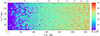Fig. 1. Light-cone of EoR 21 cm signal. This shows the redshift (z) evolution of the corresponding differential brightness temperature (δTb) from z ≈ 15.5 to 6.9. We assume a high spin temperature limit, i.e., TS ≫ Tγ. This light cone is generated using the GRIZZLY code and represents our fiducial EoR scenario.

Figure 1 shows a slice through a simulated light-cone of the EoR 21 cm signal δT_b (Eq. (1)). The figure represents how the fluctuations δT_b in the sky (shown by the vertical axis) evolve with redshift or distance from the observer (represented by the horizontal axis). Our assumption of T_S ≫ T_γ makes the H I 21 cm signal δT_b positive in the neutral regions while the ionized regions are represented by δT_b = 0. We note that ionized regions in the IGM are absent around z = 15 where the fluctuations in δT_b are governed by the density fluctuations only (Eq. (1)). Small isolated ionized regions gradually appear around the high-density peaks in δ_B. Over time, the isolated ionized regions grow in size and overlap with each other. This overlap can occur as early as when the IGM volume is ionized by a few tens of percent depending upon the reionization history. These overlaps eventually create complex percolated structures of the ionized regions which grow in volume over time as the reionization progresses. For ${\overline{x}}_{\mathrm{HI}}\gtrsim 0.5$ (i.e., z ≳ 8 in Fig. 1), the sizes of the ionized regions are smaller than the neutral regions. Visually, the ionized regions are embedded into the neutral regions. It becomes the opposite at reionization stages with ${\overline{x}}_{\mathrm{HI}}\lesssim 0.5$. At these stages, the distribution of the neutral regions is more meaningful compared to the distribution of the ionized regions.

2.2. The EoR 21 cm signal power spectrum

This study is based on the k-dependent features of the dimensionless power spectrum of coeval δT_b cube at redshift z, i.e., ${\mathrm{\Delta }}_{\delta T_{\text{b}}}^2(z,k)=k^3{P}_{\delta T_{\text{b}}}(z,k)/2{\pi }^2$ during different stages of the EoR. Assuming statistical homogeneity of the signal, one can define the 3D power spectrum for a coeval signal volume V as ${\delta }_{\mathrm{K}}(\mathit{k}-{\mathit{k}}^{\prime })P_{\delta T_{\mathrm{b}}}(z,\mathit{k})=V^{-1}⟨\widehat{\delta T_{\mathrm{b}}}(z,\mathit{k}){\widehat{\delta T_{\mathrm{b}}}}^{\ast }(z,{\mathit{k}}^{\prime })⟩$, where δ_k(k − k′) denotes the 3D Kroneker’s delta function and $\widehat{\delta T_{\mathrm{b}}}(z,\mathit{k})$ is the Fourier transform of the EoR 21 cm signal δT_b(x, z). Here we use the spherically averaged power spectrum P_δTb(z, k) which is computed by averaging P_δTb(z, k) within spherical shells of certain widths in 3D Fourier space. According to Eq. (1), the EoR 21 cm power spectrum ${\mathrm{\Delta }}_{\delta T_{\text{b}}}^2(z,k)$ depends on the power spectra of the density and neutral fraction fields (${\mathrm{\Delta }}_{\delta \delta }^2$ and ${\mathrm{\Delta }}_{x_{\text{HI}}{x}_{\text{HI}}}^2$ respectively), and their cross power spectrum ${\mathrm{\Delta }}_{x_{\text{HI}}\delta }^2$. Here, ${\mathrm{\Delta }}_{\delta \delta }^2$ is associated with a field given by Eq. (1) for x_HI(x, z) = 1, therefore powered by the density fluctuations only. On the other hand, the field associated with ${\mathrm{\Delta }}_{x_{\text{HI}}{x}_{\text{HI}}}^2$ assumes δ_B(x, z) = 0 in Eq. (1), and thus is independent of the density fluctuations and only depends on the neutral fraction fluctuations (Lidz et al. 2007; Georgiev et al. 2022)⁹. ${\mathrm{\Delta }}_{x_{\text{HI}}\delta }^2$ is the cross-power spectrum of the fields associated with ${\mathrm{\Delta }}_{\delta \delta }^2$ and ${\mathrm{\Delta }}_{x_{\text{HI}}{x}_{\text{HI}}}^2$.

Figure 2 shows the evolution of the EoR 21 cm signal power spectrum ${\mathrm{\Delta }}_{\delta T_{\text{b}}}^2$ as well as the power spectra of the density field ${\mathrm{\Delta }}_{\delta \delta }^2$, neutral fraction field ${\mathrm{\Delta }}_{x_{\text{HI}}{x}_{\text{HI}}}^2$, and their cross-power spectrum ${\mathrm{\Delta }}_{x_{\text{HI}}\delta }^2$. The power spectra correspond to our fiducial GRIZZLY EoR scenario as presented in Fig. 1. The a–d panels of Fig. 2 show ${\mathrm{\Delta }}_{\delta T_{\text{b}}}^2$, ${\mathrm{\Delta }}_{\delta \delta }^2$, ${\mathrm{\Delta }}_{x_{\text{HI}}{x}_{\text{HI}}}^2$, and $\left|{\mathrm{\Delta }}_{x_{\text{HI}}\delta }^2\right|$ respectively as a function of k at different redshifts. The panel e shows the redshift evolution of ${\mathrm{\Delta }}_{\delta T_{\text{b}}}^2$ for different scales while panel f compares the redshift evolution of the ${\mathrm{\Delta }}_{x_{\text{HI}}{x}_{\text{HI}}}^2,\hspace{0.17em}{\mathrm{\Delta }}_{\delta \delta }^2$, and $\left|{\mathrm{\Delta }}_{x_{\text{HI}}\delta }^2\right|$ for k = 0.1 h Mpc⁻¹. The high-density regions get ionized first in this inside-out reionization model. This causes anti-correlation between x_HI and δ and thus, negative values for the cross-power spectrum ${\mathrm{\Delta }}_{x_{\text{HI}}\delta }^2$ which suppresses the large-scale δT_b power spectrum at the initial stage of the EoR¹⁰. However, the suppression is less significant at the small-scales, causing a tilt in the ${\mathrm{\Delta }}_{\delta T_{\text{b}}}^2$ compared to the ${\mathrm{\Delta }}_{\delta \delta }^2$ (see panels a and b). For z ≳ 9, $\left|{\mathrm{\Delta }}_{x_{\text{HI}}\delta }^2\right|$ remains larger than ${\mathrm{\Delta }}_{x_{\text{HI}}{x}_{\text{HI}}}^2$ (see panels d and f). For z ≲ 9, ${\mathrm{\Delta }}_{x_{\text{HI}}{x}_{\text{HI}}}^2$ becomes the dominant term. The interplay between the ${\mathrm{\Delta }}_{x_{\text{HI}}{x}_{\text{HI}}}^2$ and ${\mathrm{\Delta }}_{x_{\text{HI}}\delta }^2$ contributions causes a minimum in the ${\mathrm{\Delta }}_{\delta T_{\text{b}}}^2$ vs z curves around z ∼ 10 (see bottom panels). The large-scale δT_b power spectrum increases as reionization progresses. For example, ${\mathrm{\Delta }}_{\delta T_{\mathrm{b}}}^2(k=0.1h{\mathrm{Mpc}}^{-1})$ increases from z = 9 to z = 7.3 as ${\mathrm{\Delta }}_{x_{\text{HI}}{x}_{\text{HI}}}^2$ becomes dominant compared to ${\mathrm{\Delta }}_{x_{\text{HI}}\delta }^2$. For z ≲ 7.3, ${\mathrm{\Delta }}_{\delta T_{\mathrm{b}}}^2(k=0.1h{\mathrm{Mpc}}^{-1})$ quickly drops as the majority of the IGM gets ionized. This causes ${\mathrm{\Delta }}_{\delta T_{\mathrm{b}}}^2(k=0.1h{\mathrm{Mpc}}^{-1})$ to peak at redshift 7.3 with amplitude of ≈10 mK². The peak amplitudes and the associated redshifts change with k (see panel e of Fig. 2).

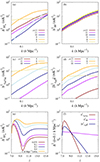Fig. 2. Power spectra of EoR 21 cm signal brightness temperature and their different components. The a–d panels show ${\mathrm{\Delta }}_{\delta T_{\text{b}}}^2,\hspace{0.17em}{\mathrm{\Delta }}_{\delta \delta }^2$, ${\mathrm{\Delta }}_{x_{\text{HI}}{x}_{\text{HI}}}^2$, and $\left|{\mathrm{\Delta }}_{x_{\text{HI}}\delta }^2\right|$ respectively as a function of k at different stages of reionization. The e panel shows the redshift evolution of the 21 cm power spectrum at different scales. The f panel compares the redshift evolution of ${\mathrm{\Delta }}_{x_{\text{HI}}{x}_{\text{HI}}}^2,\hspace{0.17em}{\mathrm{\Delta }}_{\delta \delta }^2$, and $\left|{\mathrm{\Delta }}_{x_{\text{HI}}\delta }^2\right|$ at k = 0.1 h Mpc−1. The power spectra correspond to our fiducial GRIZZLY EoR scenario as shown in Fig. 1.

The top panel of Fig. 3 shows the ratio of ${\mathrm{\Delta }}_{\delta T_{\text{b}}}^2$ to ${\mathrm{\Delta }}_{\delta \delta }^2$ (also known as the 21 cm signal bias) as a function of k at different redshifts for the fiducial GRIZZLY model. The bottom panel of Fig. 3 shows the evolution of ${\mathrm{\Delta }}_{\delta T_{\text{b}}}^2/{\mathrm{\Delta }}_{\delta \delta }^2$ for k = 0.05 h Mpc⁻¹ as a function of ${\overline{x}}_{\mathrm{HI}}$. The different curves in the bottom panels correspond to different GRIZZLY reionization models, with the thick black curve representing the fiducial one. This ratio is expected to be 1 for ${\overline{x}}_{\mathrm{HI}}=1$. The curves show that the ratio first decreases from 1 to a minimum at an early stage of reionization. We denote ${\overline{x}}_{\mathrm{HI}}$ at this stage as ${\overline{x}}_{\mathrm{HI},\min }$. This minimum corresponds to the equilibration phase caused by the anti-correlation between the density and neutral fraction fields in our inside-out reionization model where ${\mathrm{\Delta }}_{x_{\text{HI}}\delta }^2$ < 0. The ratio then increases with the increase of the size of the ionized regions and reaches a maximum and further decreases to zero as ${\overline{x}}_{\mathrm{HI}}$ approaches zero towards the end of the EoR. We denote the ionization fraction at the stage when the maximum occurs as ${\overline{x}}_{\mathrm{HI},\star }$. The qualitative features of the different curves in the bottom panel of Fig. 3 are similar, although the stages when the minimum and maximum occur (i.e., the values of ${\overline{x}}_{\mathrm{HI},\min }$ and ${\overline{x}}_{\mathrm{HI},\star }$) and the peak amplitude of the ratio ${\mathrm{\Delta }}_{\delta T_{\text{b}}}^2/{\mathrm{\Delta }}_{\delta \delta }^2$ changes with the patchiness of the reionization scenarios. The curve which reaches the largest bias or ratio value (approximately 14) corresponds to the model which uses the largest values for both M_min (10¹¹ M_⊙) and α_S (2), and thus represents the most patchy reionization scenario among the considered models. Nevertheless, the evolutionary features of this ratio as a function of ${\overline{x}}_{\mathrm{HI}}$ remain the same despite being an early or late reionization.

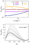Fig. 3. Ratio of ${\mathrm{\Delta }}_{\delta T_{\text{b}}}^2$ to ${\mathrm{\Delta }}_{\delta \delta }^2$ obtained from simulations during EoR. The top panel shows ${\mathrm{\Delta }}_{\delta T_{\text{b}}}^2/{\mathrm{\Delta }}_{\delta \delta }^2$ as a function of k at different redshifts. These correspond to our fiducial GRIZZLY model which is also shown in Fig. 2. The bottom panel shows evolution of ${\mathrm{\Delta }}_{\delta T_{\text{b}}}^2/{\mathrm{\Delta }}_{\delta \delta }^2$ at k = 0.05 h Mpc−1 as a function of neutral fraction. Different curves stand for different reionization scenarios generated using GRIZZLY by varying αS and Mmin. The black curve represents our fiducial GRIZZLY simulation which corresponds to αS = 1 and Mmin = 109 M⊙.

2.3. Modeling scale dependence of the EoR 21 cm signal power spectrum at a given redshift

In this section, we aim to model the complex scale dependence of the δT_b power spectrum (e.g., see Figs. 2 and 3) as we described in the previous section. The k-dependence of ${\mathrm{\Delta }}_{\delta T_{\text{b}}}^2$ evolves with redshift. It should be noted that this study considers features of the power spectrum for the range 0.05 h Mpc⁻¹ ≲ k ≲ 0.6 h Mpc⁻¹, which covers the scales probed by EoR observations such as LOFAR and MWA. The overall feature of the power spectrum, as we have seen in the top panel of Fig. 3 (see also, Xu et al. 2019; Georgiev et al. 2022), suggests that one possible ansatz to represent the k-dependence of the coeval EoR 21 cm signal power spectrum can be

$$\begin{array}{c}\hfill {\mathrm{\Delta }}_{\delta T_{\mathrm{b}}}^2(k,z)=A\frac{{\left(\frac{k}{k_c}\right)}^{\gamma }}{1+{\left(\frac{k}{k_0}\right)}^{\eta }}{\mathrm{\Delta }}_{\delta \delta }^2(k,z).\end{array}$$(2)

Here A, k_c, k₀, γ, and η are the parameters to fit ${\mathrm{\Delta }}_{\delta T_{\text{b}}}^2$ at a particular redshift, considering ${\mathrm{\Delta }}_{\delta \delta }^2$ to be known for the background cosmology. The form of the numerator in Eq. (2) is chosen to compensate for the difference in slope between ${\mathrm{\Delta }}_{\delta T_{\text{b}}}^2$ and ${\mathrm{\Delta }}_{\delta \delta }^2$ during the early stages of the EoR (see Fig. 2). On the other hand, the denominator accounts for the fall of ${\mathrm{\Delta }}_{\delta T_{\text{b}}}^2$ relative to the corresponding ${\mathrm{\Delta }}_{\delta \delta }^2$ at the small scales (e.g., for k ≳ 0.1 h Mpc⁻¹) during the advanced stages of the EoR (e.g., for ${\overline{x}}_{\mathrm{HI}}\lesssim 0.7$). For ${\overline{x}}_{\mathrm{HI}}=1$, one expects A = 1, γ = 0, k₀ → ∞ and η to be positive. It is expected that the k₀ values are much larger compared to the smallest k value achieved by the EoR H I observations. For example, LOFAR reaches k ∼ 0.05 h Mpc⁻¹ as reported in papers such as Patil et al. (2017). We set k_c = 0.05 h Mpc⁻¹ which makes the A parameter equal to the ratio of ${\mathrm{\Delta }}_{\delta T_{\text{b}}}^2$ to ${\mathrm{\Delta }}_{\delta \delta }^2$ at k = 0.05 h Mpc⁻¹ if k₀ is quite large compared to 0.05 h Mpc⁻¹.

We first attempt to fit the power spectra at different redshifts using Eq. (2), separately, by varying A,  k₀,  γ, and η on a grid for our fiducial GRIZZLY scenario. We explore the log(A), γ, log(k₀), and η parameter space on equal-spaced grids. The chosen parameter ranges are [ − 4, 2], [ − 2, 2], [ − 1, 0], and [0, 3], respectively. We estimate the best-fit values of these four parameters at each redshift by minimizing the error

$$\begin{array}{c}\hfill {\mathrm{\Psi }}_4^2(\mathcal{S}:[z,A,\gamma ,k_0,\eta ])=\frac{1}{n}{\displaystyle \sum _{i=1,n}}{\left(\frac{{\mathrm{\Delta }}_{\delta T_{\mathrm{b}},m}^2(\mathcal{S})}{{\mathrm{\Delta }}_{\delta T_{\mathrm{b}},o}^2(z,k_i)}-1\right)}^2.\end{array}$$

We consider a k range in between 0.05 and 0.6 h Mpc⁻¹ and divide it into n = 9 log spaced bins. Here, ${\mathrm{\Delta }}_{\delta T_{\text{b}},m}^2$ represents the modeled power spectrum using Eq. (2) for a set of input parameters. ${\mathrm{\Delta }}_{\delta T_{\text{b}},o}^2$ is the observed or input power spectrum which we consider for fitting. The evolution of the best-fit parameter values as a function of ${\overline{x}}_{\mathrm{HI}}$ is shown in the different panels of Fig. 4. The rightmost panel, which shows the goodness of the fit, indicates that the maximum error in our fitting is well within 10%.

Fig. 4. Outcome of fitting EoR power spectra using Eq. (2). Left to right panels show the evolution of the best-fit values of the parameters A, γ, k0 and η and fitting error as a function of ${\overline{x}}_{\mathrm{HI}}$ for different reionization scenarios generated using GRIZZLY. Bold lines correspond to the fiducial GRIZZLY reionization scenario.

The left panel of Fig. 4 presents the best-fit values of A as a function of ${\overline{x}}_{\mathrm{HI}}$. These roughly agree with the values presented in Fig. 3. We find that k₀ reaches the maximum value of the range or becomes unconstrained (simultaneously η becomes ill-defined) during the early stages of reionization (${\overline{x}}_{\mathrm{HI}}\ge {\overline{x}}_{\mathrm{HI},\min }$) before significant overlap between the isolated ionized regions occurs. Eventually, the formation of large overlapped ionized regions changes the k dependencies on the small-scale power spectra. With the growth of overlapping ionized regions, the characteristic bubble size increases, which implies a decrease in k₀ values while remaining much larger than 0.05 h Mpc⁻¹. We repeated the fitting of Eq. (2) for our different GRIZZLY scenarios and found a qualitatively similar dependence of k₀ and η on reionization history (see grey lines in Fig. 4).

It is expected from Eq. (2) that the parameters γ, k₀, and η might be degenerate. To reduce degenerate parameters and to minimize the number of parameters in our ansatz, we fix k₀ and η at typical values of the best-fit parameters throughout the reionization history. We fixed η = 1.5, while we fixed k₀ = 0.3 h Mpc⁻¹ for ${\overline{x}}_{\mathrm{HI}}\lesssim {\overline{x}}_{\mathrm{HI},\min }$ and infinity otherwise. This reduces the number of parameters and modifies Eq. (2) to

$$\begin{array}{c}\hfill {\mathrm{\Delta }}_{\delta T_{\mathrm{b}}}^2=\{\begin{array}{cc}{\mathrm{\Delta }}_{\delta \delta }^{2}A\frac{{\left(\frac{k}{0.05}\right)}^{\gamma }}{1+{\left(\frac{k}{0.3}\right)}^{1.5}},\hfill & \mathrm{if}{\overline{x}}_{\mathrm{HI}}\lesssim {\overline{x}}_{\mathrm{HI},\min }.\hfill \\ {\mathrm{\Delta }}_{\delta \delta }^{2}A{\left(\frac{k}{0.05}\right)}^{\gamma },\hfill & \mathrm{otherwise}.\hfill \end{array}\end{array}$$(3)

As before, we fixed k_c to 0.05, which ensures that the parameter A represents the ratio ${\mathrm{\Delta }}_{\delta T_{\text{b}}}^2/{\mathrm{\Delta }}_{\delta \delta }^2$ at k = 0.05 h Mpc⁻¹.

To check the performance of the form in Eq. (3), we vary the parameters A and γ and compare the fitted power spectrum ${\mathrm{\Delta }}_{\delta T_{\text{b}},m}^2(z,k,A,\gamma )$ with the simulated input power spectrum ${\mathrm{\Delta }}_{\delta T_{\text{b}},o}^2(z,k)$ at each redshift independently. We explore the log(A) and γ parameter space on grids where we have chosen the same parameter ranges as above, i.e., [ − 4, 2] and [ − 2, 2], respectively. We estimate the best-fit values of A and γ at each redshifts by minimizing the error

$$\begin{array}{c}\hfill {\mathrm{\Psi }}_2^2(z,A,\gamma )=\frac{1}{n}{\displaystyle \sum _{i=1,n}}{\left(\frac{{\mathrm{\Delta }}_{\delta T_{\mathrm{b}},m}^2(z,k_i,A,\gamma )}{{\mathrm{\Delta }}_{\delta T_{\mathrm{b}},o}^2(z,k_i)}-1\right)}^2.\end{array}$$

The two left panels of Fig. 5 present the evolution of the best-fit values of A and γ as a function of ${\overline{x}}_{\mathrm{HI}}$ for different GRIZZLY reionization scenarios. The right panel of the figure presents Ψ₂ × 100 as a function of ${\overline{x}}_{\mathrm{HI}}$. The figure shows that, even with the simplified form of ${\mathrm{\Delta }}_{\delta T_{\text{b}}}^2$ as used in Eq. (3), the fitting error Ψ₂ is ≲10% and not drastically different compared to Ψ₄. On the other hand, the evolution of the γ parameter is now smoother compared to the four-parameter case.

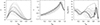Fig. 5. Outcome of fitting EoR power spectra using Eq. (3). Left to right panels show the evolution of the best-fit values of the parameters A and γ and fitting error as a function of ${\overline{x}}_{\mathrm{HI}}$ for different reionization scenarios. It should be noted that here we have used Eq. (3) while we used Eq. (2) for Fig. 4. The reionization scenarios are the same as in Fig. 4. Bold lines correspond to the fiducial GRIZZLY reionization scenario.

The top panel of Fig. 6 shows a comparison between the power spectrum of our fiducial reionization scenario and its best-fit power spectrum ${\mathrm{\Delta }}_{\delta T_{\text{b}},f}^2(z,k)$ obtained using Eq. (3). The bottom panel of Fig. 6 shows the percentage fitting error Err$({\mathrm{\Delta }}_{\delta T_{\mathrm{b}}}^2)=(1-\frac{{\mathrm{\Delta }}_{\delta T_{\mathrm{b}},f}^2}{{\mathrm{\Delta }}_{\delta T_{\mathrm{b}}}^2})\times 100\%$ as a function of k modes for the different redshifts. The plot shows that Eq. (3) can predict the power spectrum of the fiducial EoR scenario with error ≲10%. We roughly find similar results for other GRIZZLY reionization scenarios.

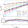Fig. 6. Comparing simulated and fitted EoR power spectra using Eq. (3). The top panel shows a comparison between the 21 cm signal power spectrum of our fiducial reionization scenario and its best-fit power spectrum obtained using Eq. (3). Different colors represent different redshifts. The lines correspond to the power spectrum ${\mathrm{\Delta }}_{\delta T_{\text{b}}}^2$ from GRIZZLY simulations while the points stand for the fitted power spectrum ${\mathrm{\Delta }}_{\delta T_{\text{b}},f}^2$. The bottom panel shows the percentage fitting error Err$({\mathrm{\Delta }}_{\delta T_{\mathrm{b}}}^2)=(1-\frac{{\mathrm{\Delta }}_{\delta T_{\mathrm{b}},f}^2}{{\mathrm{\Delta }}_{\delta T_{\mathrm{b}}}^2})\times 100\%$.

2.4. Modeling the redshift evolution of the EoR 21 cm signal power spectrum

We already find that the form of the 21 cm power spectrum as used in Eq. (3) works well for different stages of reionization. However, for any given reionization scenario, the best-fit values of the A and γ evolve with redshift or alternatively ${\overline{x}}_{\mathrm{HI}}$. Thus, it is important to understand the behavior of A and γ parameters as a function of ${\overline{x}}_{\mathrm{HI}}$ to come up with a final set of redshift-independent parameters which can be constrained using multi-redshift EoR 21 cm signal power spectra measurements.

The left panel of Fig. 5 shows the dependencies of the best-fit values of A as a function of ${\overline{x}}_{\mathrm{HI}}$. We note that both the bottom panel of Fig. 3 and the left panel of Fig. 5 represent the evolution of ${\mathrm{\Delta }}_{\delta T_{\text{b}}}^2/{\mathrm{\Delta }}_{\delta \delta }^2$ at k = 0.05 h Mpc⁻¹ as a function of ${\overline{x}}_{\mathrm{HI}}$. While the curves in the bottom panel of Fig. 3 show the estimates directly from the GRIZZLY simulation, the curves in the left panel of Fig. 5 represent the best-fit value of parameter A when using Eq. (3) for modeling ${\mathrm{\Delta }}_{\delta T_{\text{b}}}^2$. A = 1 when ${\overline{x}}_{\mathrm{HI}}=1$ and the 21 cm signal power spectrum is completely determined by density fluctuations. As reionization progresses (i.e., ${\overline{x}}_{\mathrm{HI}}$ deceases), A first decreases and reaches its minimum value at ${\overline{x}}_{\mathrm{HI}}={\overline{x}}_{\mathrm{HI},\min }$. Thereafter, A increases until ${\overline{x}}_{\mathrm{HI}}={\overline{x}}_{\mathrm{HI},\star }$ where it reaches a maximum value, which we call A_⋆. After this, A decreases and A → 0 for ${\overline{x}}_{\mathrm{HI}}\to 0$ when reionization ends.

We model the dependence of A on ${\overline{x}}_{\mathrm{HI}}$ in the following way.

$$\begin{array}{c}\hfill A=A_{\star }{\left(\frac{{\overline{x}}_{\mathrm{HI}}}{{\overline{x}}_{\mathrm{HI},\star }}\right)}^{{\alpha }_A}{\left(\frac{1-{\overline{x}}_{\mathrm{HI}}}{1-{\overline{x}}_{\mathrm{HI},\star }}\right)}^{{\beta }_A}+{10}^{-5\times (1-{\overline{x}}_{\mathrm{HI}})}\end{array}$$(4)

with ${\beta }_A={\alpha }_A(1-{\overline{x}}_{\mathrm{HI},\star })/{\overline{x}}_{\mathrm{HI},\star }$. In Eq. (4), ${\overline{x}}_{\mathrm{HI},\star },A_{\star }$, and the slope α_A are free parameters that set the evolution of A as a function of ${\overline{x}}_{\mathrm{HI}}$. The reionization scenarios considered in this study suggest ${\overline{x}}_{\mathrm{HI},\star }\lesssim 0.5$. The first term of the right hand side in the above equation shows the ${\overline{x}}_{\mathrm{HI}}$ dependence of ${\mathrm{\Delta }}_{\delta T_{\text{b}}}^2/{\mathrm{\Delta }}_{\delta \delta }^2$ at k = 0.05 h Mpc⁻¹ for stages when the ionization power spectrum (${\mathrm{\Delta }}_{x_{\text{HI}}{x}_{\text{HI}}}^2$) dominates the 21 cm signal power spectrum in comparison with the matter density. The second part of the right hand side of this equation shows the ${\overline{x}}_{\mathrm{HI}}$ dependence during the initial stages of the EoR corresponding to ${\overline{x}}_{\mathrm{HI}}>{\overline{x}}_{\mathrm{HI},\min }$ when the density power spectrum (${\mathrm{\Delta }}_{\delta \delta }^2$) and the anti-correlation between the density and neutral fraction (${\mathrm{\Delta }}_{x_{\text{HI}}\delta }^2$) are important (see, e.g., Fig. 2). We note that the second term rapidly decreases as ${\overline{x}}_{\mathrm{HI}}$ decreases and is negligible at the stages when the peak of A vs ${\overline{x}}_{\mathrm{HI}}$ curves occurs. Thus, we neglect the second term when we determine the values for β_A in terms of α_A at the maximum. Deriving an analytical form for ${\overline{x}}_{\mathrm{HI},\min }$ is not straightforward, as we estimate ${\overline{x}}_{\mathrm{HI},\min }$ numerically for a set of our input parameters and thus ${\overline{x}}_{\mathrm{HI},\min }$ is a derived quantity for a given model.

Next, we check the accuracy of the fitting form of A as used in Eq. (4). We consider the evolution of $A={\mathrm{\Delta }}_{\delta T_{\mathrm{b}}}^2/{\mathrm{\Delta }}_{\delta \delta }^2(k=0.05h{\mathrm{Mpc}}^{-1})$ as a function of ${\overline{x}}_{\mathrm{HI}}$ from different GRIZZLY reionization scenarios as inputs. We vary $A_{\star },{\overline{x}}_{\mathrm{HI},\star }$, and α_A on regularly spaced grids respectively in the ranges [0, 20], [0, 1], and [0, 2], and determine their best-fit values. For a particular reionization scenario, we fit the evolution of A values corresponding to different stages of reionization together using Eq. (4). The top panel of Fig. 7 shows the best-fit values of the parameters A_⋆, ${\overline{x}}_{\mathrm{HI},\star }$, and α_A. Although we observe a clear correlation between A_⋆ and ${\overline{x}}_{\mathrm{HI},\star }$, as A is sensitive to small changes in these parameters, we still keep all of them as independent parameters in our final ansatz. The bottom panel of Fig. 7 shows the evolution of A − A_f as a function of ${\overline{x}}_{\mathrm{HI}}$ for different GRIZZLY reionization scenarios. Here, A_f represents the best-fit value of A obtained using Eq. (4).

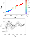Fig. 7. Results of fitting the dependence of A on ${\overline{x}}_{\mathrm{HI}}$ using Eq. (4). Top panel shows the best-fit values of the parameters A⋆, ${\overline{x}}_{\mathrm{HI},\star }$ and αA when we fit different curves of the left panel of Fig. 5 using Eq. (4). Here, A represents the ratio ${\mathrm{\Delta }}_{\delta T_{\text{b}}}^2/{\mathrm{\Delta }}_{\delta \delta }^2$ at k ∼ 0.05 h Mpc−1. The bottom panel shows the difference between the input/true A values and predicted (or fitted) Af values with the best-fit parameters as a function of average ionization fraction ${\overline{x}}_{\mathrm{HI}}$.

Next, we consider the γ parameter. The middle panel of Fig. 5 shows the dependencies of the best-fit values of γ on ${\overline{x}}_{\mathrm{HI}}$. As expected, γ → 0 for ${\overline{x}}_{\mathrm{HI}}\to 1$. For ${\overline{x}}_{\mathrm{HI}}>{\overline{x}}_{\mathrm{HI},\min }$, γ increases as ${\overline{x}}_{\mathrm{HI}}$ decreases and roughly shows a power-law dependency on ${\overline{x}}_{\mathrm{HI}}$. We modeled this part as $\gamma ={10}^{-2}{\overline{x}}_{\mathrm{HI}}^{{\gamma }_p}$ where γ_p is the power-law index. For ${\overline{x}}_{\mathrm{HI}}\lesssim {\overline{x}}_{\mathrm{HI},\min }$, γ decreases with ${\overline{x}}_{\mathrm{HI}}$ and roughly shows an exponential drop while γ reaches negative values for ${\overline{x}}_{\mathrm{HI}}\to 0$. We modeled this drop of γ with the decreases of ${\overline{x}}_{\mathrm{HI}}$ as $\gamma ={\gamma }_{1}exp[{\gamma }_c{\overline{x}}_{\mathrm{HI}}]+{\gamma }_0$. The parameter γ_c controls the rate of decrease of γ for ${\overline{x}}_{\mathrm{HI}}\lesssim {\overline{x}}_{\mathrm{HI},\min }$, while γ₀ + γ₁ represents γ values when ${\overline{x}}_{\mathrm{HI}}\to 0$. Therefore we choose the fitting form for γ to be written as

$$\begin{array}{cc}\hfill \gamma =& ({\gamma }_{1}exp[{\gamma }_c{\overline{x}}_{\mathrm{HI}}]+{\gamma }_0)(1-\mathcal{H}({\overline{x}}_{\mathrm{HI},\min }))\hfill \\ \hfill & +{10}^{-2}{\overline{x}}_{\mathrm{HI}}^{{\gamma }_p}\mathcal{H}({\overline{x}}_{\mathrm{HI},\min }),\hfill \end{array}$$(5)

where, ℋ is the Heaviside step function. In order to reduce the number of parameters, we use a boundary condition for γ. As the two discontinuous functional forms of γ for ${\overline{x}}_{\mathrm{HI}}\le {\overline{x}}_{\mathrm{HI},\min }$ and ${\overline{x}}_{\mathrm{HI}}>{\overline{x}}_{\mathrm{HI},\min }$ have the same value for ${\overline{x}}_{\mathrm{HI}}={\overline{x}}_{\mathrm{HI},\min }$, we can determine γ_p as ${\gamma }_p=log({\gamma }_{1}exp[{\gamma }_c{\overline{x}}_{\mathrm{HI},\min }]+{\gamma }_0)/(0.01log{\overline{x}}_{\mathrm{HI},\min })$.

Next, we check the accuracy of the fitting form of γ as defined in Eq. (5). We consider different evolutions of γ as a function of ${\overline{x}}_{\mathrm{HI}}$ from the middle panel of Fig. 5. We vary γ₀, log γ₁, and γ_c on regularly spaced grids respectively in the ranges [ − 1.5, 0], [ − 3, 0], and [0, 10] and determine their best-fit values. Note that the fitting considers different γ values corresponding to different stages of a particular reionization history to obtain the best-fit values. The top panel of Fig. 8 shows the best-fit values of the parameters γ₁, γ_c, and γ₀. The bottom panel of Fig. 8 shows the deviation γ − γ_f as a function of ${\overline{x}}_{\mathrm{HI}}$ for different GRIZZLY reionization scenarios. Here, γ_f represents the γ value for the best-fit value of the parameters following Eq. (5). Similarly to the fit for A, here we find a prominent correlation between γ_c and γ₁. As γ_c and log γ₁ behave roughly linearly, we consider γ₁ = 10^{(1.3 − γ_c)/2.25} which r5educes the number of parameters to γ_c and γ₀. Here, γ_c accounts for the change in k-dependence of the bias ${\mathrm{\Delta }}_{\delta T_{\text{b}}}^2/{\mathrm{\Delta }}_{\delta \delta }^2$ with ${\overline{x}}_{\mathrm{HI}}$ for ${\overline{x}}_{\mathrm{HI}}\le {\overline{x}}_{\mathrm{HI},\min }$. γ₀ accounts for the power-law dependence on k feature of ${\mathrm{\Delta }}_{\delta T_{\text{b}}}^2/{\mathrm{\Delta }}_{\delta \delta }^2$ in addition to small-scale feature 1/[1 + (k/0.3)^1.5] at stages when ${\overline{x}}_{\mathrm{HI}}\to 0$.

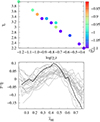Fig. 8. Results of fitting the dependence of γ on ${\overline{x}}_{\mathrm{HI}}$ using Eq. (5). Top panel shows the best-fit values of the parameters log γ1, γc, and γ0 when we fit different curves in the middle panel of Fig. 5 using Eq. (5). The bottom panel shows the difference between the input or true γ values and predicted/fitted γf values with the best-fit parameters as a function of average ionization fraction ${\overline{x}}_{\mathrm{HI}}$.

Now, we are left with an ansatz which depends on five redshift-independent parameters $A_{\star },{\overline{x}}_{\mathrm{HI},\star },{\alpha }_A,{\gamma }_c$, and γ₀ to model the EoR 21 cm power spectrum as a function of k modes and the reionization history, which is parametrized by the globally averaged neutral fraction ${\overline{x}}_{\mathrm{HI}}(z)$. In the following section, we introduce our modeling of reionization history.

2.5. Modeling the reionization history

The EoR 21 cm signal observations with radio interferometers are initially going to produce power spectrum ${\mathrm{\Delta }}_{\delta T_{\text{b}}}^2(z,k)$ at different redshifts z. However, our ansatz (Eqs. (3)–(5)) predicts ${\mathrm{\Delta }}_{\delta T_{\text{b}}}^2$ as a function of k and ${\overline{x}}_{\mathrm{HI}}$. Therefore, it is necessary to model the reionization history ${\overline{x}}_{\mathrm{HI}}$ as a function of redshift z.

The top panel of Fig. 9 shows the redshift evolution of the volume-averaged neutral fraction ${\overline{x}}_{\mathrm{HI}}$ for all the GRIZZLY reionization scenarios considered in this work. We find ${\overline{x}}_{\mathrm{HI}}\approx 1$ for z ≳ 11 while the bulk of reionization occurs within a narrow redshift window (Δz ≲ 4) at z ≲ 11. We note that the reionization histories are asymmetric around ${\overline{x}}_{\mathrm{HI}}=0.5$. There is no well-established analytical form which accurately represents the redshift evolution of ${\overline{x}}_{\mathrm{HI}}$. One possible analytical form to represent the asymmetric redshift evolution of ${\overline{x}}_{\mathrm{HI}}$ is (e.g., Heinrich et al. 2017)

$$\begin{array}{c}\hfill \begin{array}{cc}& {\overline{x}}_{\mathrm{HI}}(z_0,{\alpha }_0,\mathrm{\Delta }z,z)=\frac{1}{2}[1-tanh\left\{\frac{y(z_0)-y(z)}{\mathrm{\Delta }y}\right\}],\hfill \\ \hfill & \mathrm{where}y(z)={(1+z)}^{{\alpha }_0},\hfill \\ \hfill & \mathrm{and}\mathrm{\Delta }y={\alpha }_0{(1+z)}^{{\alpha }_0-1}\times \mathrm{\Delta }z.\hfill \end{array}\end{array}$$(6)

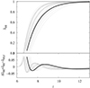Fig. 9. Modeling of reionization history ${\overline{x}}_{\mathrm{HI}}(z)$ using Eq. (6). The top panel shows the evolution of the neutral fraction as a function of redshift for different reionization scenarios generated using GRIZZLY code. The bold black curve corresponds to our GRIZZLY fiducial reionization scenario. The bottom panel shows fitting error $\mathrm{\Delta }{\overline{x}}_{\mathrm{HI}}={\overline{x}}_{\mathrm{HI}}-{\overline{x}}_{\mathrm{HI},\mathrm{f}}$ on the redshift evolution of ${\overline{x}}_{\mathrm{HI}}$. We have used an asymmetric tanh function (see Eq. (6)) to model the redshift evolution of ${\overline{x}}_{\mathrm{HI}}$.

Here z₀, Δz, and α₀ are free parameters which govern the evolution of the mean neutral fraction ${\overline{x}}_{\mathrm{HI}}$ with z₀ representing the redshift at which ${\overline{x}}_{\mathrm{HI}}=0.5$, Δz the duration of the reionization, and α₀ the asymmetry of reionization history around z₀. We note that the parametrization of ${\overline{x}}_{\mathrm{HI}}$ as a function of redshift is not unique. Here, we have used an analytically simpler form for ${\overline{x}}_{\mathrm{HI}}(z)$. An alternative parametrization of the reionization history such as the one used in Trac (2018) could also produce a good fit to the reionization scenarios used in this study.

The bottom panel of Fig. 9 shows the fitting error $\mathrm{\Delta }{\overline{x}}_{\mathrm{HI}}=({\overline{x}}_{\mathrm{HI}}-{\overline{x}}_{\mathrm{HI},\mathrm{f}})$ between the simulated (${\overline{x}}_{\mathrm{HI}}$) and best-fit (${\overline{x}}_{\mathrm{HI},\mathrm{f}}$) values of the reionization histories. The best-fit ionization history for a given simulated reionization scenario is obtained by varying z₀, Δz, and α₀ on uniformly spaced grids and minimizing the mean square error

$$\begin{array}{c}\hfill E_{\mathrm{tot}}(z_0,\mathrm{\Delta }z,{\alpha }_0)=\frac{1}{n_z}{\displaystyle \sum _{z<15.5}}{[{\overline{x}}_{\mathrm{HI}}(z_0,{\alpha }_0,\mathrm{\Delta }z,z)-{\overline{x}}_{\mathrm{HI}}(z)]}^2.\end{array}$$

Here n_z is the number of redshifts considered for a reionization history, which can differ for different EoR models of GRIZZLY. We vary z₀, Δz, and α₀ in the range [5, 15], [0, 3], and [0, 10] ranges, respectively. All the GRIZZLY reionization scenarios show a good fit with $\mathrm{\Delta }{\overline{x}}_{\mathrm{HI}}\lesssim 0.03$ for the majority of the reionization redshifts ranges. At the same time, the error increases up to ∼0.08 near the end of EoR when ${\overline{x}}_{\mathrm{HI}}\to 0$. This shows that a tanh form has some trouble capturing the fast drop in ${\overline{x}}_{\mathrm{HI}}$ during the tail end of the reionization.

In Sect. 2.4, we used five redshift-independent parameters to model the scale dependence of ${\mathrm{\Delta }}_{\delta T_{\text{b}}}^2$ as a function of ${\overline{x}}_{\mathrm{HI}}$. In this section, we used three z independent parameters to model the redshift evolution of ${\overline{x}}_{\mathrm{HI}}$. Thus in the end, we are left with a set of eight redshift-independent free parameters $\mathit{\theta }=[z_0,\mathrm{\Delta }z,{\alpha }_0,A_{\star },{\overline{x}}_{\mathrm{HI},\star },{\alpha }_A,{\gamma }_c,{\gamma }_0]$ to model both the scale dependence and redshift evolution of the EoR 21 cm power spectrum together with the reionization history. See Table 1 for a description of the parameters.

3. Results

We next apply our eight-parameter ansatz of the EoR 21 cm power spectra to various reionization scenarios obtained from different simulations. As inputs, we consider a C2RAY, a 21CMFAST, and all the GRIZZLY simulations as mentioned in the previous section. These three 21 cm simulation frameworks are based on very different source models, but to be consistent with our ansatz for ${\mathrm{\Delta }}_{\delta T_{\text{b}}}^2$, we assume T_S ≫ T_γ in all of them. We refer the readers to Ghara et al. (2015a), Mellema et al. (2006), and Mesinger et al. (2011) for the details of the algorithms used in these three simulations.

From each reionization scenario, we extract power spectra for eight different redshifts covering the majority of the EoR. The redshift ranges for C2RAY, 21CMFAST, and GRIZZLY scenarios are [6.1, 9], [6.4, 9.6], and [7.1, 11.1] respectively. Figure 10 shows the redshift evolution of ${\overline{x}}_{\mathrm{HI}}$ (left column) and the corresponding simulated EoR 21 cm signal power spectra (right column) for the C2RAY (top row), 21CMFAST (middle row), and the fiducial GRIZZLY scenario (bottom row). The redshifts of these power spectra span ∼60 MHz of observational bandwidth while the frequency difference between two adjacent redshifts is Δν ∼ 7 MHz. The latter is smaller than the typical bandwidth used in EoR 21 cm data analysis. For example, Mertens et al. (2020) used 12 MHz bandwidth to estimate the upper limits on the 21 cm power spectrum at redshift 9.1. The main motivation to use a smaller bandwidth is to resolve the fast evolving nature of the large-scale power spectrum around the peak. However, the choice of a smaller bandwidth will need more observation hours to reach the same signal-to-noise ratio.

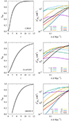Fig. 10. Three different input reionization histories and power spectra which are used to check the performance of our ansatz. The top, middle and bottom panels correspond to C2RAY, 21CMFAST, and GRIZZLY fiducial input reionization scenarios. The left panels show the redshift evolution of ${\overline{x}}_{\mathrm{HI}}$ while the right panels show the set of input power spectra used in the MCMC analysis.

Next we use these power spectra to constrain the eight parameters of our ansatz using Markov chain Monte Carlo (MCMC) based parameter estimation framework. We use the publicly available code COSMOMC¹¹ (Lewis & Bridle 2002) for exploring the log-likelihood of these eight parameters θ. The log-likelihood in our MCMC algorithm is estimated as,

$$\begin{array}{c}\hfill {\chi }^2(\mathit{\theta })=-{\displaystyle \sum _{i,j}}{\left(\frac{{\mathrm{\Delta }}_{\delta T_{\mathrm{b}},m}^2(z_i,k_j,\mathit{\theta })-{\mathrm{\Delta }}_{\delta T_{\mathrm{b}},o}^2(z_i,k_j)}{{\mathrm{\Delta }}_{\mathrm{o},\mathrm{err}}^2}\right)}^2,\end{array}$$

where ${\mathrm{\Delta }}_{\delta T_{\text{b}},m}^2$ and ${\mathrm{\Delta }}_{\delta T_{\text{b}},o}^2$ are the modeled and the simulated input power spectra, respectively. The index i runs over the eight input redshifts while the index j runs over k-bins with 0.05 h Mpc⁻¹ ≤ k ≤ 0.6 h Mpc⁻¹. Each MCMC analysis here is done with 8 independent walkers (sequences of parameter values in MCMC), each of which takes 10⁶ steps.

The quantity ${\mathrm{\Delta }}_{\text{o},\text{err}}^2$ in the denominator is the error used in our MCMC analysis. In principle, this error should include measurement error, sample variance, and the imperfection of the ansatz. However, as the aim is to show a proof of concept of our ansatz, we consider the simple case in which the error ${\mathrm{\Delta }}_{\text{o},\text{err}}^2$ = 1 mK² is k and z independent. In general, ${\mathrm{\Delta }}_{\text{o},\text{err}}^2$ is expected to increase towards higher redshifts. Considering any observation, the scale dependence of ${\mathrm{\Delta }}_{\text{o},\text{err}}^2$ changes with redshift as the uv coverage of an interferometric observation changes with observation frequency and also the sky noise varies with the frequency. Here, we do not consider such realistic situations and will address these issues in a follow-up work.

We run the MCMC analysis on the C2RAY, 21CMFAST, and GRIZZLY scenarios. The input power spectra for each scenario are presented in Fig. 10. The outcomes of the MCMC analysis are presented in the following subsections.

3.1. Scenario I: C2RAY

First, we consider a reionization scenario which is generated using the EoR 21 cm signal modeling code C2RAY (Mellema et al. 2006). This code uses the gridded density field and halo lists from N-body simulations and applies “Conservative Causal Ray-tracing method” based 3D radiative transfer to produce ionization fraction fields at different stages of reionization. The set of δT_b power spectra and the redshift evolution of ${\overline{x}}_{\mathrm{HI}}$ of the input reionization history as obtained from a C2RAY simulation are shown in the top row of Fig. 10. This scenario uses the same dark-matter fields and halo list as used in the GRIZZLY simulations. C2RAY also considers contributions from all dark-matter halos with their masses larger than 10⁹ M_⊙ and assumes the rate of production of the ionizing photons to be 1.3 × 10⁴² × M_halo/M_⊙ s⁻¹. In this simulation, the mean-free-path length of the ionizing photons is chosen as 70 Mpc. In this C2RAY reionization scenario, ${\overline{x}}_{\mathrm{HI}}$ decreases from 0.9 to 0 as reionization progressed between z ≈ 8 and 6. We find that the evolution of the ratio ${\mathrm{\Delta }}_{\delta T_{\text{b}}}^2/{\mathrm{\Delta }}_{\delta \delta }^2$ at k = 0.05 h Mpc⁻¹ reaches a maximum value of ≈5 at z ≈ 6.4 when ${\overline{x}}_{\mathrm{HI}}\approx 0.3$.

Figure 11 shows the posteriors of the eight parameters θ of our power spectrum ansatz when we use the set of C2RAY power spectra as inputs to our MCMC framework. The off-diagonal panels show the joint probability distribution for a pair of parameters where 2D contours represent 1σ and 2σ confidence levels respectively. The curves in the diagonal panels represent the marginalized probability distributions of the individual ansatz parameters. The plot shows that while most of the parameters are well-constrained, some of them are not. One reason behind this might be the degeneracy of these parameters with the other parameters. The best-fit parameter values obtained from this analysis are z₀ = 6.9, Δz = 0.83, α₀ = 6.4, A_⋆ = 5.2, ${\overline{x}}_{\mathrm{HI},\star }=0.27$, α_A = 1.8, γ_c = 2, and γ₀ = −1.2 (see also Table 2). The best-fit values of A_⋆ and ${\overline{x}}_{\mathrm{HI},\star }$ agree well with the input reionization scenario which corresponds to A_⋆ = 5.01 and ${\overline{x}}_{\mathrm{HI},\star }=0.22$. The comparison between input and best-predicted models for this reionization scenario is shown in the left column of Fig. 12. Here The top-left panel shows the comparison as a function of k at different redshifts while the middle-left panel shows the redshift evolution of the predicted and input ratio ${\mathrm{\Delta }}_{\delta T_{\text{b}}}^2/{\mathrm{\Delta }}_{\delta \delta }^2$ for different k-bins. The curves indicate that our ansatz performs well at different stages of the reionization and for the k range we considered here. A comparison between the input reionization history and the ansatz predictions (bottom-left panel of Fig. 12) suggests an excellent recovery of the redshift evolution of ${\overline{x}}_{\mathrm{HI}}$ using our model. Figure 13 shows the corresponding deviation ${\overline{x}}_{\mathrm{HI}}-{\overline{x}}_{\mathrm{HI},\mathrm{best}-\mathrm{fit}}$ where ${\overline{x}}_{\mathrm{HI},\mathrm{best}-\mathrm{fit}}$ represents the prediction using the MCMC best-fit parameters. Here, we find that the deviation remains between ±0.05 as indicated by the blue thick curve.

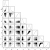Fig. 11. Posterior of the ansatz parameters (see Table 1). This shows the constraints of the fiducial EoR scenario obtained using the MCMC analysis in terms of the EoR power spectrum model parameters. The contours in the two-dimensional contour plots represent 1σ and 2σ confidence levels respectively. The curves in the diagonal panels are the marginalized probability distributions of the eight parameters. The MCMC analysis is performed on inputs from C2RAY.

3.2. Scenario II: 21CMFAST

Our second input reionization scenario is generated using the publicly available semi-numerical 21 cm code 21CMFAST (Mesinger et al. 2011; Park et al. 2019). In this semi-numerical approach, the density fields are generated following the first-order perturbation theory (Zel’dovich 1970) while the ionization fields are produced using the excursion-set approach (Furlanetto et al. 2004). We assume the following parameters: fraction of galactic gas in stars for 10¹⁰ M_⊙ halo f_⋆, 10 = 0.05, the power-law index for star formation and halo mass relation α_⋆ = 0.5, the UV ionizing escape fraction for 10¹⁰ M_⊙ halo f_esc, 10 = 0.1, the power-law index for UV escape fraction and halo mass relation α_esc = −0.5, the characteristic mass scale for star formation suppression M_turn = 5 × 10⁸ M_⊙, star-formation timescale in units of the Hubble time t_⋆ = 0.5, number of ionizing photons per stellar baryon N_γ = 5000, and mean-free path of ionizing photons R_mfp = 50 Mpc (for the details of these parameters, see Park et al. 2019). In this case, reionization ends at z ∼ 6 while the majority of the ionization happens below z ≲ 10. The corresponding input reionization history and the input power spectra are shown in the middle row of Fig. 10. The input set of the 21 cm power spectra of the reionization scenario shows features similar to those of the fiducial GRIZZLY and C2RAY scenarios. We find that the ratio ${\mathrm{\Delta }}_{\delta T_{\text{b}}}^2/{\mathrm{\Delta }}_{\delta \delta }^2$ at k = 0.05 h Mpc⁻¹ reaches a maximum value of ≈1.3 at z ≈ 7.2 corresponding to ${\overline{x}}_{\mathrm{HI}}=0.35$.

We repeat the MCMC analysis (as done for C2RAY) to obtain the posterior of our ansatz parameters. The middle row of Table 2 shows the posterior constraints on the eight parameters of our ansatz. The best-fit parameter values are z₀ = 7.7, Δz = 1.7, α₀ = 5.5, A_⋆ = 1.6, ${\overline{x}}_{\mathrm{HI},\star }=0.38$, α_A = 1.9, γ_c = 3.5, and γ₀ = −0.8. The corresponding power spectra predictions at all the redshifts agree well with the input simulated power spectra (see the top and middle panels of the central column of Fig. 12). Similar to the previous case, the best-fit values of A_⋆ and ${\overline{x}}_{\mathrm{HI},\star }$ agree well with the input 21CMFAST reionization scenario which has A_⋆ = 1.3 and ${\overline{x}}_{\mathrm{HI},\star }=0.34$. We compare the simulated reionization history ${\overline{x}}_{\mathrm{HI}}(z)$ with that predicted from our MCMC analysis in the bottom-central panel of Fig. 12. Similar to the C2RAY scenario, our framework works efficiently in this case as well and recovers reionization history ${\overline{x}}_{\mathrm{HI}}$ within a maximum deviation between ±0.03 as shown by the orange line in Fig. 13.

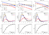Fig. 12. Comparison between the input reionization scenario and recovered model from the MCMC analysis using EoR power spectra as input to the phenomenological model considered in this work. Left to right columns represent C2RAY, 21CMFAST, and GRIZZLY simulation respectively. From top to bottom we show, respectively, the ratio of 21 cm signal to density power spectrum (${\mathrm{\Delta }}_{\delta T_{\text{b}}}^2/{\mathrm{\Delta }}_{\delta \delta }^2$) as a function of k-scales at different redshifts, the redshift evolution of ${\mathrm{\Delta }}_{\delta T_{\text{b}}}^2/{\mathrm{\Delta }}_{\delta \delta }^2$ for different scales and the corresponding reionization histories. The solid curves represent the inputs from simulations while the dotted curves stand for the MCMC best-fit prediction on the power spectrum model used in this work.

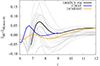Fig. 13. Redshift evolution of the difference between the input model neutral fraction and best-fit neutral fraction. The MCMC analysis here considers our eight-parameter model for the EoR power spectra. Different thin grey curves stand for different reionization scenarios from GRIZZLY simulation. The black curve represents our fiducial GRIZZLY simulation while the blue and orange curves present C2RAY and 21CMFAST input scenarios. The best-fit parameter values are obtained using input power spectra at eight redshifts for each reionization scenario.

3.3. Scenario III: GRIZZLY

The simulated input power spectra and the reionization history for the fiducial GRIZZLY reionization scenario are shown in the bottom panels of Fig. 10. As described in Sect. 2.1, this corresponds to GRIZZLY parameters ζ = 1, M_min = 10⁹ M_⊙, and α_S = 1 (for details, see Ghara et al. 2020). This results in a reionization history where the IGM gets 10% ionized at z ≈ 11 while the reionization ends around z ≈ 7 (see top right panel of Fig. 12). Here, the ratio ${\mathrm{\Delta }}_{\delta T_{\text{b}}}^2/{\mathrm{\Delta }}_{\delta \delta }^2$ at k = 0.05 h Mpc⁻¹ reaches a maximum value of ≈6 at z ≈ 7.3 which corresponds to ${\overline{x}}_{\mathrm{HI}}=0.25$.

The posterior constraints on the ansatz parameters, obtained using MCMC analysis, are summarized in the bottom row of Table 2. The best-fit parameter values are z₀ = 8.1, Δz = 1.2, α₀ = 6.6, A_⋆ = 5.2, ${\overline{x}}_{\mathrm{HI},\star }=0.24$, α_A = 1.3, γ_c = 2.4, and γ₀ = −0.88. Similar to the previous cases, the predicted power spectra and the best-fit values of A_⋆ and ${\overline{x}}_{\mathrm{HI},\star }$ are in good agreement with the simulated input values. The A_⋆ and ${\overline{x}}_{\mathrm{HI},\star }$ values from the input reionization scenario are 5.8 and 0.22, respectively. The predicted evolution of ${\overline{x}}_{\mathrm{HI}}$ as shown in the top right panel of Fig. 12 shows good agreement within the absolute deviations of 0.05.

We repeat our MCMC analysis for the other 23 GRIZZLY models as represented by the shaded grey lines in Figs. 9 and 3 considering the input power spectra at the same redshifts used for the fiducial GRIZZLY model. We plot the difference between the input and predicted neutral fraction for all these models in Fig. 13. These suggest that our ansatz represents the EoR 21 cm power spectrum close enough and can recover the reionization history ${\overline{x}}_{\mathrm{HI}}(z)$ within an absolute error of ∼0.1 (see the grey lines in Fig. 13). We note that the evolution of ${\overline{x}}_{\mathrm{HI}}$ as a function of redshift is very steep around z₀ and thus even a small error in the estimate of z₀ will result in a large difference between the input (true) and predicted ${\overline{x}}_{\mathrm{HI}}$. This is evident from the plots for various GRIZZLY models in Fig. 13 between redshift 7 and 8. The deviations could become larger for the models having steeper slopes around z₀.

4. Summary and conclusions

The redshifted 21 cm signal from the IGM during the EoR encodes unique information about that period. The 21 cm observations indirectly probe the properties of the ionizing and heating sources and directly probes the ionization and thermal states of the IGM during the first billion years of our Universe. In this study, we focus on inferring the properties of the EoR IGM, rather than those of astrophysical sources, through 21 cm signal observations. The large-scale amplitude and scale-dependent features of the EoR 21 cm brightness temperature power spectrum depend on the ionization fraction of hydrogen and the morphology and distribution of the ionized or neutral regions. Our main aim is to develop a source parameter-free phenomenological model that constrains the properties of the EoR IGM using multi-redshift 21 cm power spectrum measurements. The framework constrains the redshift evolution of the average neutral fraction and a set of quantities related to the morphology and distribution of the ionized regions.

Using different GRIZZLY simulations, we study the scale-dependent features of the 21 cm power spectra at different stages of EoR. The quantity we aim to model is the ratio of the 21 cm brightness temperature (δT_b) to the density power spectrum also known as the 21 cm bias in the literature. We modeled this ratio as ${\mathrm{\Delta }}_{\delta T_{\mathrm{b}}}^2/{\mathrm{\Delta }}_{\delta \delta }^2=A\frac{{\left(\frac{k}{0.05}\right)}^{\gamma }}{1+{\left(\frac{k}{0.3}\right)}^{1.5}}$. Here, A represents bias at k = 0.05 h Mpc⁻¹. We tested the goodness of fit of our ansatz at various stages of reionization using 24 different GRIZZLY scenarios. These tests suggest that the aforementioned functional form of the ratio of δT_b to density power spectra efficiently reproduce the EoR 21 cm power spectra for different reionization histories, accurately within ≲10% error (see Fig. 6).

As the A and γ parameters in the above-mentioned ansatz evolve during reionization, we additionally model how these parameters evolve as a function of ${\overline{x}}_{\mathrm{HI}}$. The model for A (Eq. (4)) uses three parameters, the maximum value of the ratio (A_⋆), the corresponding neutral fraction ${\overline{x}}_{\mathrm{HI},\star }$, and a power-law index α_A. The evolution of γ can be described with two parameters (Eq. (5)): γ_c which accounts for the change in scale-dependence, and γ₀ which accounts for the deviation of the scale dependence of ${\mathrm{\Delta }}_{\delta T_{\text{b}}}^2/{\mathrm{\Delta }}_{\delta \delta }^2$ from 1/[1 + (k/0.3)^1.5] at small-scales (see Sect. 2.4 for details).

Using the GRIZZLY simulations, we fit the evolution of ${\overline{x}}_{\mathrm{HI}}$ as a function of redshift using three parameters (see Eq. (6)). These are: redshift z₀ which corresponds to ${\overline{x}}_{\mathrm{HI}}=0.5$, redshift range of reionization Δz in a tanh reionization model, and asymmetry parameter α₀ to invoke asymmetry in history around ${\overline{x}}_{\mathrm{HI}}=0.5$. We tested the goodness of this form of ${\overline{x}}_{\mathrm{HI}}(z)$ using 24 different GRIZZLY reionization models and found them to be consistent within $\mathrm{\Delta }{\overline{x}}_{\mathrm{HI}}=\pm 0.1$ (see Fig. 9).

In the end, we are left with a set of eight redshift and scale-independent parameters $\mathit{\theta }=[z_0,\mathrm{\Delta }z,{\alpha }_0,A_{\star },{\overline{x}}_{\mathrm{HI},\star },{\alpha }_A,{\gamma }_c,{\gamma }_0]$ to jointly model the redshift evolution and scale-dependence of the ratio ${\mathrm{\Delta }}_{\delta T_{\text{b}}}^2/{\mathrm{\Delta }}_{\delta \delta }^2$. We demonstrate the performance of this ansatz with 24 GRIZZLY models, one reionization scenario from C2RAY and one from 21CMFAST. We use as an input the power spectra simulated at eight redshifts within the interval z = [7.1 − 11.1] (corresponds to ∼60 MHz bandwidth) and perform a Bayesian MCMC analysis to constrain the ansatz parameters for each of the three reionization scenarios. All these tests collectively indicate that our ansatz reproduces the scale-dependence and the redshift evolution of the ratio ${\mathrm{\Delta }}_{\delta T_{\text{b}}}^2/{\mathrm{\Delta }}_{\delta \delta }^2$ reasonably well for a variety of reionization models considered here. The predicted redshift evolution of ${\overline{x}}_{\mathrm{HI}}$, using the best-fit MCMC parameter set θ, matches nicely with the input reionization history within $\mathrm{\Delta }{\overline{x}}_{\mathrm{HI}}=\pm 0.1$ (see Fig. 13). At the same time the constrained values for $A_{\star },{\overline{x}}_{\mathrm{HI},\star }$ match closely with the reionization scenarios (see Fig. 12 and Table 2).

Our aforementioned approach is similar in spirit to a few previous studies. For example, Battaglia et al. (2013) simulate a reionization redshift field for a given density field (filtered at a particular scale). However, their approach fundamentally assumes a strong correlation between the density and reionization redshift fields. On the other hand, McQuinn & D’Aloisio (2018) take a perturbative approach to construct an EoR 21 cm signal field using the underlying density field. Their formalism assumes some source field and patchiness-dependent bias factors as well as a characteristic size of ionized regions to connect the 21 cm signal field with the density field. Unlike them, our approach is conceptually simpler and directly connects the EoR 21 cm signal power spectrum with the matter power spectrum. This phenomenological model directly exploits the features of multi-redshift EoR 21 cm signal power spectra for predicting the quantities related to the EoR IGM states. Thus, it makes our ansatz more flexible, computationally inexpensive and faster while exploring IGM parameters in the context of current and future observations. Additionally, our phenomenological ansatz is agnostic to the various methods of EoR simulations (3D and 1D radiative transfer and excursion-set based), whereas the analysis in Mirocha et al. (2022) is restricted to the excursion-set based simulations only.

The analysis presented in this paper is only based on the “inside-out” reionization scenario where the highly dense regions around the radiating sources become ionized first. We speculate that the same is also applicable for an “outside-in” reionization model as the scale-dependence of the EoR power spectra as well as the redshift evolution of the large-scale power spectrum are qualitatively similar to the “inside-out” case for the wavenumber range of our interest (see e.g., Figs. 2 and 3 of Pagano & Liu 2020). However, in the “outside-in” case, we do not expect a trough of the large-scale power spectra at ${\overline{x}}_{\mathrm{HI},\min }$ and thus we expect an even simpler form of the ansatz for the EoR power spectra. We leave a detailed investigation for the “outside-in” reionization scenario for a future study.

The accuracy of the ansatz predictions of the EoR 21 cm power spectra suggests that it will be useful to constrain reionization scenarios using existing and upcoming measurements from LOFAR, MWA, HERA, and SKA. Here, we have used a simple-minded constant error on the input power spectra. It will be interesting to see the performance of this model when realistic errors are taken into account. We plan to address this in our future work.

Our model is based on δT_b power spectra with high spin temperatures. This model also works if the gas temperature of the neutral IGM remains uniform. However, things get complicated when the presence of spin temperature fluctuations modifies the power spectra significantly. One expects a more complex evolution of the power spectrum in that case. Modeling such behaviors is out of the scope of this paper and will be addressed in a follow-up work.

Here we consider only the EoR 21 cm power spectra measurements to constrain the reionization history. In addition, information from several other probes such as the Thomson scattering optical depth measurement from CMB observation (e.g., Planck Collaboration VI 2020), the Gunn-Peterson trough in high-z quasar spectra (e.g., Fan et al. 2006; Becker et al. 2015), observations of high-z Ly-α emitters (e.g., Hu et al. 2010; Morales et al. 2021), and the Ly-α damping wings in high-z quasar spectra (e.g., Bañados et al. 2018) can also be combined with the H I measurements from the EoR to tighten the constrain on the reionization history. We plan to address this in a future study using POLAR (Ma et al. 2023) algorithm which is based on GRIZZLY and the semi-analytical galaxy formation code L-Galaxies 2020 and self-consistently model the evolution of galaxy properties during the EoR.

Although our framework is efficient in recovering the redshift evolution of the average ionization fraction using the measurements of the EoR 21 cm signal power spectrum, there are several aspects that need improvements. While most of the parameters of this framework are easy to interpret, understanding the physical meaning of a few parameters such as γ_c and γ₀ is non-trivial. These parameters are connected to the morphology and distribution of the ionized regions. It is important to understand how these quantities are linked to the distribution of morphological quantities such as volume, surface, and mean curvature (see, e.g., Giri et al. 2018; Giri & Mellema 2021; Ghara et al. 2024). This study is also beyond the scope of this work. We plan to address it in a future study.

Acknowledgments

R.G., A.K.S., and S.Z. acknowledge support from the Israel Science Foundation (grant no. 255/18). Furthermore, R.G. acknowledges support from the Kaufman Foundation (Gift no. GF01364). S.Z. also acknowledges Alexander von Humboldt Foundation for the Humboldt Research award. A.K.S. also acknowledges support from National Science Foundation (grant no. 2206602). G.M. acknowledges support by the Swedish Research Council grant 2020-04691. L.V.E.K. acknowledges the financial support from the European Research Council (ERC) under the European Union’s Horizon 2020 research and innovation programme (Grant agreement No. 884760, “CoDEX”).

References

All Tables

All Figures

	Fig. 1. Light-cone of EoR 21 cm signal. This shows the redshift (z) evolution of the corresponding differential brightness temperature (δTb) from z ≈ 15.5 to 6.9. We assume a high spin temperature limit, i.e., TS ≫ Tγ. This light cone is generated using the GRIZZLY code and represents our fiducial EoR scenario.
In the text

Fig. 2. Power spectra of EoR 21 cm signal brightness temperature and their different components. The a–d panels show ${\mathrm{\Delta }}_{\delta T_{\text{b}}}^2,\hspace{0.17em}{\mathrm{\Delta }}_{\delta \delta }^2$, ${\mathrm{\Delta }}_{x_{\text{HI}}{x}_{\text{HI}}}^2$, and $\left|{\mathrm{\Delta }}_{x_{\text{HI}}\delta }^2\right|$ respectively as a function of k at different stages of reionization. The e panel shows the redshift evolution of the 21 cm power spectrum at different scales. The f panel compares the redshift evolution of ${\mathrm{\Delta }}_{x_{\text{HI}}{x}_{\text{HI}}}^2,\hspace{0.17em}{\mathrm{\Delta }}_{\delta \delta }^2$, and $\left|{\mathrm{\Delta }}_{x_{\text{HI}}\delta }^2\right|$ at k = 0.1 h Mpc−1. The power spectra correspond to our fiducial GRIZZLY EoR scenario as shown in Fig. 1.

In the text

Fig. 3. Ratio of ${\mathrm{\Delta }}_{\delta T_{\text{b}}}^2$ to ${\mathrm{\Delta }}_{\delta \delta }^2$ obtained from simulations during EoR. The top panel shows ${\mathrm{\Delta }}_{\delta T_{\text{b}}}^2/{\mathrm{\Delta }}_{\delta \delta }^2$ as a function of k at different redshifts. These correspond to our fiducial GRIZZLY model which is also shown in Fig. 2. The bottom panel shows evolution of ${\mathrm{\Delta }}_{\delta T_{\text{b}}}^2/{\mathrm{\Delta }}_{\delta \delta }^2$ at k = 0.05 h Mpc−1 as a function of neutral fraction. Different curves stand for different reionization scenarios generated using GRIZZLY by varying αS and Mmin. The black curve represents our fiducial GRIZZLY simulation which corresponds to αS = 1 and Mmin = 109 M⊙.

In the text

	Fig. 4. Outcome of fitting EoR power spectra using Eq. (2). Left to right panels show the evolution of the best-fit values of the parameters A, γ, k0 and η and fitting error as a function of ${\overline{x}}_{\mathrm{HI}}$ for different reionization scenarios generated using GRIZZLY. Bold lines correspond to the fiducial GRIZZLY reionization scenario.
In the text

Fig. 5. Outcome of fitting EoR power spectra using Eq. (3). Left to right panels show the evolution of the best-fit values of the parameters A and γ and fitting error as a function of ${\overline{x}}_{\mathrm{HI}}$ for different reionization scenarios. It should be noted that here we have used Eq. (3) while we used Eq. (2) for Fig. 4. The reionization scenarios are the same as in Fig. 4. Bold lines correspond to the fiducial GRIZZLY reionization scenario.

In the text

Fig. 6. Comparing simulated and fitted EoR power spectra using Eq. (3). The top panel shows a comparison between the 21 cm signal power spectrum of our fiducial reionization scenario and its best-fit power spectrum obtained using Eq. (3). Different colors represent different redshifts. The lines correspond to the power spectrum ${\mathrm{\Delta }}_{\delta T_{\text{b}}}^2$ from GRIZZLY simulations while the points stand for the fitted power spectrum ${\mathrm{\Delta }}_{\delta T_{\text{b}},f}^2$. The bottom panel shows the percentage fitting error Err$({\mathrm{\Delta }}_{\delta T_{\mathrm{b}}}^2)=(1-\frac{{\mathrm{\Delta }}_{\delta T_{\mathrm{b}},f}^2}{{\mathrm{\Delta }}_{\delta T_{\mathrm{b}}}^2})\times 100\%$.

In the text

Fig. 7. Results of fitting the dependence of A on ${\overline{x}}_{\mathrm{HI}}$ using Eq. (4). Top panel shows the best-fit values of the parameters A⋆, ${\overline{x}}_{\mathrm{HI},\star }$ and αA when we fit different curves of the left panel of Fig. 5 using Eq. (4). Here, A represents the ratio ${\mathrm{\Delta }}_{\delta T_{\text{b}}}^2/{\mathrm{\Delta }}_{\delta \delta }^2$ at k ∼ 0.05 h Mpc−1. The bottom panel shows the difference between the input/true A values and predicted (or fitted) Af values with the best-fit parameters as a function of average ionization fraction ${\overline{x}}_{\mathrm{HI}}$.

In the text

References

- Abdurashidova, T. H. C. Z., Adams, T., Aguirre, J. E., et al. 2023, ApJ, 945, 124 [NASA ADS] [CrossRef] [Google Scholar]
- Abdurashidova, Z., Aguirre, J. E., Alexander, P., et al. 2022a, ApJ, 924, 51 [NASA ADS] [CrossRef] [Google Scholar]
- Abdurashidova, Z., Aguirre, J. E., Alexander, P., et al. 2022b, ApJ, 925, 221 [NASA ADS] [CrossRef] [Google Scholar]
- Bañados, E., Venemans, B. P., Mazzucchelli, C., et al. 2018, Nature, 553, 473 [Google Scholar]
- Barkana, R. 2018, Nature, 555, 71 [Google Scholar]
- Battaglia, N., Trac, H., Cen, R., & Loeb, A. 2013, ApJ, 776, 81 [NASA ADS] [CrossRef] [Google Scholar]
- Becker, G. D., Bolton, J. S., Madau, P., et al. 2015, MNRAS, 447, 3402 [Google Scholar]
- Becker, G. D., Davies, F. B., Furlanetto, S. R., et al. 2018, ApJ, 863, 92 [NASA ADS] [CrossRef] [Google Scholar]
- Bera, A., Ghara, R., Chatterjee, A., Datta, K. K., & Samui, S. 2023, JApA, 44, 10 [Google Scholar]
- Bonaldi, A., & Brown, M. L. 2015, MNRAS, 447, 1973 [NASA ADS] [CrossRef] [Google Scholar]
- Bowman, J. D., Rogers, A. E. E., Monsalve, R. A., Mozdzen, T. J., & Mahesh, N. 2018, Nature, 555, 67 [Google Scholar]
- Chapman, E., Zaroubi, S., Abdalla, F. B., et al. 2016, MNRAS, 458, 2928 [NASA ADS] [CrossRef] [Google Scholar]
- Chatterjee, A., Dayal, P., Choudhury, T. R., & Hutter, A. 2019, MNRAS, 487, 3560 [NASA ADS] [CrossRef] [Google Scholar]
- Chatterjee, A., Dayal, P., Choudhury, T. R., & Schneider, R. 2020, MNRAS, 496, 1445 [NASA ADS] [CrossRef] [Google Scholar]
- Cohen, A., Fialkov, A., Barkana, R., & Monsalve, R. A. 2020, MNRAS, 495, 4845 [NASA ADS] [CrossRef] [Google Scholar]
- Datta, K. K., Bharadwaj, S., & Choudhury, T. R. 2007, MNRAS, 382, 809 [NASA ADS] [CrossRef] [Google Scholar]
- Datta, A., Bowman, J. D., & Carilli, C. L. 2010, ApJ, 724, 526 [NASA ADS] [CrossRef] [Google Scholar]
- de Lera Acedo, E., de Villiers, D. I. L., Razavi-Ghods, N., et al. 2022, Nat. Astron., 6, 984 [NASA ADS] [CrossRef] [Google Scholar]
- DeBoer, D. R., Parsons, A. R., Aguirre, J. E., et al. 2017, PASP, 129, 045001 [NASA ADS] [CrossRef] [Google Scholar]
- Eide, M. B., Ciardi, B., Graziani, L., et al. 2020, MNRAS, 498, 6083 [Google Scholar]
- Eilers, A.-C., Davies, F. B., & Hennawi, J. F. 2018, ApJ, 864, 53 [NASA ADS] [CrossRef] [Google Scholar]
- Ewall-Wice, A., Hewitt, J., Mesinger, A., et al. 2016, MNRAS, 458, 2710 [NASA ADS] [CrossRef] [Google Scholar]
- Fan, X., Strauss, M. A., Becker, R. H., et al. 2006, AJ, 132, 117 [NASA ADS] [CrossRef] [Google Scholar]
- Fialkov, A., Barkana, R., & Cohen, A. 2018, Phys. Rev. Lett., 121, 011101 [NASA ADS] [CrossRef] [Google Scholar]
- Furlanetto, S. R., Zaldarriaga, M., & Hernquist, L. 2004, ApJ, 613, 1 [NASA ADS] [CrossRef] [Google Scholar]
- Furlanetto, S. R., Oh, S. P., & Briggs, F. H. 2006, Phys. Rep., 433, 181 [Google Scholar]
- Gan, H., Koopmans, L. V. E., Mertens, F. G., et al. 2022, A&A, 663, A9 [NASA ADS] [CrossRef] [EDP Sciences] [Google Scholar]
- Gan, H., Mertens, F. G., Koopmans, L. V. E., et al. 2023, A&A, 669, A20 [NASA ADS] [CrossRef] [EDP Sciences] [Google Scholar]
- Gehlot, B. K., Koopmans, L. V. E., Offringa, A. R., et al. 2022, A&A, 662, A97 [NASA ADS] [CrossRef] [EDP Sciences] [Google Scholar]
- Georgiev, I., Mellema, G., Giri, S. K., & Mondal, R. 2022, MNRAS, 513, 5109 [NASA ADS] [CrossRef] [Google Scholar]
- Ghara, R., & Mellema, G. 2020, MNRAS, 492, 634 [NASA ADS] [CrossRef] [Google Scholar]
- Ghara, R., Choudhury, T. R., & Datta, K. K. 2015a, MNRAS, 447, 1806 [NASA ADS] [CrossRef] [Google Scholar]
- Ghara, R., Datta, K. K., & Choudhury, T. R. 2015b, MNRAS, 453, 3143 [Google Scholar]
- Ghara, R., Choudhury, T. R., & Datta, K. K. 2016, MNRAS, 460, 827 [NASA ADS] [CrossRef] [Google Scholar]
- Ghara, R., Choudhury, T. R., Datta, K. K., & Choudhuri, S. 2017, MNRAS, 464, 2234 [NASA ADS] [CrossRef] [Google Scholar]
- Ghara, R., Giri, S. K., Mellema, G., et al. 2020, MNRAS, 493, 4728 [NASA ADS] [CrossRef] [Google Scholar]
- Ghara, R., Giri, S. K., Ciardi, B., Mellema, G., & Zaroubi, S. 2021, MNRAS, 503, 4551 [NASA ADS] [CrossRef] [Google Scholar]
- Ghara, R., Mellema, G., & Zaroubi, S. 2022, JCAP, 2022, 055 [CrossRef] [Google Scholar]
- Ghara, R., Bag, S., Zaroubi, S., & Majumdar, S. 2024, MNRAS, 530, 191 [NASA ADS] [CrossRef] [Google Scholar]
- Ghosh, A., Prasad, J., Bharadwaj, S., Ali, S. S., & Chengalur, J. N. 2012, MNRAS, 426, 3295 [NASA ADS] [CrossRef] [Google Scholar]
- Giri, S. K., & Mellema, G. 2021, MNRAS, 505, 1863 [NASA ADS] [CrossRef] [Google Scholar]
- Giri, S. K., Mellema, G., & Ghara, R. 2018, MNRAS, 479, 5596 [NASA ADS] [CrossRef] [Google Scholar]
- Giri, S. K., D’Aloisio, A., Mellema, G., et al. 2019, JCAP, 2019, 058 [Google Scholar]
- Greig, B., Mesinger, A., Koopmans, L. V. E., et al. 2021, MNRAS, 501, 1 [Google Scholar]
- Harker, G., Zaroubi, S., Bernardi, G., et al. 2009, MNRAS, 397, 1138 [NASA ADS] [CrossRef] [Google Scholar]
- Heinrich, C. H., Miranda, V., & Hu, W. 2017, Phys. Rev. D, 95, 023513 [NASA ADS] [CrossRef] [Google Scholar]
- Hinshaw, G., Larson, D., Komatsu, E., et al. 2013, ApJS, 208, 19 [Google Scholar]
- Hothi, I., Chapman, E., Pritchard, J. R., et al. 2021, MNRAS, 500, 2264 [Google Scholar]
- Hu, E. M., Cowie, L. L., Barger, A. J., et al. 2010, ApJ, 725, 394 [Google Scholar]
- Islam, N., Ghara, R., Paul, B., Choudhury, T. R., & Nath, B. B. 2019, MNRAS, 487, 2785 [NASA ADS] [CrossRef] [Google Scholar]
- Kamran, M., Ghara, R., Majumdar, S., et al. 2021, MNRAS, 502, 3800 [NASA ADS] [CrossRef] [Google Scholar]
- Kern, N. S., Parsons, A. R., Dillon, J. S., et al. 2019, ApJ, 884, 105 [NASA ADS] [CrossRef] [Google Scholar]
- Kern, N. S., Parsons, A. R., Dillon, J. S., et al. 2020, ApJ, 888, 70 [NASA ADS] [CrossRef] [Google Scholar]
- Kolopanis, M., Jacobs, D. C., Cheng, C., et al. 2019, ApJ, 883, 133 [NASA ADS] [CrossRef] [Google Scholar]
- Lewis, A., & Bridle, S. 2002, Phys. Rev. D, 66, 103511 [Google Scholar]
- Lidz, A., Zahn, O., McQuinn, M., et al. 2007, ApJ, 659, 865 [NASA ADS] [CrossRef] [Google Scholar]
- Liu, A., Parsons, A. R., & Trott, C. M. 2014, Phys. Rev. D, 90, 023019 [NASA ADS] [CrossRef] [Google Scholar]
- Ma, Q.-B., Ghara, R., Ciardi, B., et al. 2023, MNRAS, 522, 3284 [NASA ADS] [CrossRef] [Google Scholar]
- Madau, P., Meiksin, A., & Rees, M. J. 1997, ApJ, 475, 429 [NASA ADS] [CrossRef] [Google Scholar]
- McGreer, I. D., Mesinger, A., & D’Odorico, V. 2015, MNRAS, 447, 499 [NASA ADS] [CrossRef] [Google Scholar]
- McQuinn, M., & D’Aloisio, A. 2018, JCAP, 2018, 016 [CrossRef] [Google Scholar]
- Mellema, G., Iliev, I. T., Pen, U.-L., & Shapiro, P. R. 2006, MNRAS, 372, 679 [NASA ADS] [CrossRef] [Google Scholar]
- Mellema, G., Koopmans, L., Shukla, H., et al. 2015, Advancing Astrophysics with the Square Kilometre Array (AASKA14), 10 [Google Scholar]
- Mertens, F. G., Ghosh, A., & Koopmans, L. V. E. 2018, MNRAS, 478, 3640 [NASA ADS] [Google Scholar]
- Mertens, F. G., Mevius, M., Koopmans, L. V. E., et al. 2020, MNRAS, 493, 1662 [Google Scholar]
- Mesinger, A., Furlanetto, S., & Cen, R. 2011, MNRAS, 411, 955 [Google Scholar]
- Mevius, M., Mertens, F., Koopmans, L. V. E., et al. 2022, MNRAS, 509, 3693 [Google Scholar]
- Mirocha, J., Harker, G. J. A., & Burns, J. O. 2013, ApJ, 777, 118 [NASA ADS] [CrossRef] [Google Scholar]
- Mirocha, J., Muñoz, J. B., Furlanetto, S. R., Liu, A., & Mesinger, A. 2022, MNRAS, 514, 2010 [NASA ADS] [CrossRef] [Google Scholar]
- Mitra, S., Choudhury, T. R., & Ferrara, A. 2015, MNRAS, 454, L76 [NASA ADS] [CrossRef] [Google Scholar]
- Mondal, R., Fialkov, A., Fling, C., et al. 2020, MNRAS, 498, 4178 [NASA ADS] [CrossRef] [Google Scholar]
- Morales, A. M., Mason, C. A., Bruton, S., et al. 2021, ApJ, 919, 120 [CrossRef] [Google Scholar]
- Muñoz, J. B., & Loeb, A. 2018, Nature, 557, 684 [Google Scholar]
- Munshi, S., Mertens, F. G., Koopmans, L. V. E., et al. 2024, A&A, 681, A62 [NASA ADS] [CrossRef] [EDP Sciences] [Google Scholar]
- Nebrin, O., Ghara, R., & Mellema, G. 2019, JCAP, 2019, 051 [CrossRef] [Google Scholar]
- Pagano, M., & Liu, A. 2020, MNRAS, 498, 373 [NASA ADS] [CrossRef] [Google Scholar]
- Park, J., Mesinger, A., Greig, B., & Gillet, N. 2019, MNRAS, 484, 933 [NASA ADS] [CrossRef] [Google Scholar]
- Parsons, A. R., Liu, A., Aguirre, J. E., et al. 2014, ApJ, 788, 106 [NASA ADS] [CrossRef] [Google Scholar]
- Patil, A. H., Yatawatta, S., Koopmans, L. V. E., et al. 2017, ApJ, 838, 65 [NASA ADS] [CrossRef] [Google Scholar]
- Planck Collaboration VI. 2020, A&A, 641, A6 [NASA ADS] [CrossRef] [EDP Sciences] [Google Scholar]
- Price, D. C., Greenhill, L. J., Fialkov, A., et al. 2018, MNRAS, 478, 4193 [NASA ADS] [Google Scholar]
- Pritchard, J. R., & Furlanetto, S. R. 2007, MNRAS, 376, 1680 [NASA ADS] [CrossRef] [Google Scholar]
- Pritchard, J. R., & Loeb, A. 2012, Rep. Progr. Phys., 75, 086901 [CrossRef] [Google Scholar]
- Ross, H. E., Dixon, K. L., Ghara, R., Iliev, I. T., & Mellema, G. 2019, MNRAS, 487, 1101 [NASA ADS] [CrossRef] [Google Scholar]
- Ross, H. E., Giri, S. K., Mellema, G., et al. 2021, MNRAS, 506, 3717 [NASA ADS] [CrossRef] [Google Scholar]
- Shaw, A. K., Bharadwaj, S., & Mondal, R. 2020, MNRAS, 498, 1480 [CrossRef] [Google Scholar]
- Shaw, A. K., Chakraborty, A., Kamran, M., et al. 2023a, JApA, 44, 4 [Google Scholar]
- Shaw, A. K., Ghara, R., Zaroubi, S., et al. 2023b, MNRAS, 522, 2188 [NASA ADS] [CrossRef] [Google Scholar]
- Shimabukuro, H., Mao, Y., & Tan, J. 2022, Res. Astron. Astrophys., 22, 035027 [CrossRef] [Google Scholar]
- Singh, S., Subrahmanyan, R., Udaya Shankar, N., et al. 2017, ApJ, 845, L12 [NASA ADS] [CrossRef] [Google Scholar]
- Thomas, R. M., & Zaroubi, S. 2011, MNRAS, 410, 1377 [NASA ADS] [CrossRef] [Google Scholar]
- Tingay, S. J., Goeke, R., Bowman, J. D., et al. 2013, PASA, 30, 7 [Google Scholar]
- Trac, H. 2018, ApJ, 858, L11 [NASA ADS] [CrossRef] [Google Scholar]
- Trott, C. M., Jordan, C. H., Midgley, S., et al. 2020, MNRAS, 493, 4711 [NASA ADS] [CrossRef] [Google Scholar]
- van Haarlem, M. P., Wise, M. W., Gunst, A. W., et al. 2013, A&A, 556, A2 [NASA ADS] [CrossRef] [EDP Sciences] [Google Scholar]
- Wayth, R. B., Tingay, S. J., Trott, C. M., et al. 2018, PASA, 35, 33 [Google Scholar]
- Xu, W., Xu, Y., Yue, B., et al. 2019, MNRAS, 490, 5739 [Google Scholar]
- Zaroubi, S. 2013, in The First Galaxies, eds. T. Wiklind, B. Mobasher, & V. Bromm, Astrophys. Space Sci. Lib., 396, 45 [NASA ADS] [CrossRef] [Google Scholar]
- Zel’dovich, Y. B. 1970, A&A, 5, 84 [NASA ADS] [Google Scholar]
All Tables
List and description of the eight parameters used to model the redshift evolution of the EoR 21 cm brightness temperature power spectrum .
Summary of the outputs from the MCMC analysis and constraints on the eight parameter models of the EoR power spectra.