| Issue |
A&A
Volume 700, August 2025
|
|
|---|---|---|
| Article Number | A233 | |
| Number of page(s) | 22 | |
| Section | Celestial mechanics and astrometry | |
| DOI | https://doi.org/10.1051/0004-6361/202450579 | |
| Published online | 21 August 2025 | |
Translational–rotational couplings in the dynamics of Phobos
1
Royal Observatory of Belgium,
Ringlaan 3,
1180
Brussels,
Belgium
2
Delft university of Technology,
Kluyverweg 1,
Delft
2629HS,
The Netherlands
3
European Space Research and Technology Centre, ESA,
Keplerlaan 1,
Noordwijk
2201AZ,
The Netherlands
★ Corresponding author.
Received:
1
May
2024
Accepted:
18
June
2025
Abstract
Context. Upcoming science missions to Phobos will potentially provide unprecedented observations of Phobos’s orbit in the form of orbiter and/or lander tracking data. This will likely require an updating of the dynamical models currently used to invert this data, with the coupling between the satellite’s orbit and rotation being of particular importance. State-of-the-art ephemerides estimations for tidally locked satellites rely on a decoupled approach where translational models are combined with a simplified analytical representation of the moon’s rotation (typically a single-frequency periodic variation superimposed to a synchronous rotation).
Aims. This paper investigates the coupled propagation of Phobos’s translational and rotational dynamics, and assesses the extent to which the most commonly used uncoupled model can emulate the results of the coupled integration, and what consequences the mis-modeling has on the products of data inversion.
Methods. We considered two models: a coupled model that propagates Phobos’s translational and rotational dynamics simultaneously, and an uncoupled model that assumes Phobos to be in a fully locked configuration with a once-per-orbit longitudinal libration. By simulating the dynamics for about ten years, first in a coupled and then in an uncoupled manner, we compared the results and used the coupled trajectory as simulated observations for an estimation of the different parameters using uncoupled translational dynamics.
Results. For identical initial states, differences between the coupled and uncoupled trajectories were found to accumulate to 40 m, most predominantly in Phobos’s direction of motion. Longitudinal librations were misrepresented by the uncoupled model particularly around the frequencies of the normal mode, where forcings are amplified up to 3.6 × 10⁻³ degrees. Long-term latitudinal librations also arise from forcings due to coupling-induced changes in orbital inclination. The use of uncoupled models in data inversion results in true errors in the estimated parameters. In this case, we performed estimations of different lengths up to 1000 days to estimate Phobos’s initial state, once-per-orbit libration amplitude, and harmonic coefficients Ċ2,0 and Ċ2,2. Errors in dynamical parameters were found to be on the order of 10−3 degrees for the physical libration amplitude and of 10−5 for the harmonic coefficients (relative errors of around 0.1%).
Conclusions. These true errors are one to three orders of magnitude above the formal errors expected from laser ranging measurements to a Phobos lander, which indicates that the typical single-frequency uncoupled model is not suitable for the proper inversion of such data. Refined rotation models will therefore be required, either by expanding the uncoupled model to multiple frequencies or by performing a fully coupled orbital-rotational propagation as proposed in this paper. We discuss the theoretical and practical limitations of an extended analytical parametrization in the specific case of tidally locked satellites, and advocate for the use of a fully coupled approach.
Key words: methods: numerical / celestial mechanics / ephemerides / proper motions / planets and satellites: general
© The Authors 2025
 Open Access article, published by EDP Sciences, under the terms of the Creative Commons Attribution License (https://creativecommons.org/licenses/by/4.0), which permits unrestricted use, distribution, and reproduction in any medium, provided the original work is properly cited.
This article is published in open access under the Subscribe to Open model. This email address is being protected from spambots. You need JavaScript enabled to view it. to support open access publication.
1 Introduction
The two Martian moons, Phobos and Deimos, are the only natural satellites in our Solar System – together with our own – that orbit a terrestrial planet. Discovered by Hall (1878), they were repeatedly observed from Earth during the following years (e.g., Pickering et al. 1879; Keeler 1888; Newall 1895), and they were found to be in (quasi-)equatorial and (quasi-)circular orbits (Marth 1879; Woolard 1944). This suggested that the two moons formed in Mars’ proto-planetary disk. However, observations from the first Martian orbiters revealed Phobos to have a very low albedo (Smith 1970), with Phobos’s surface composition very similar to that of a carbonaceous chondrite (Veverka 1978). This was indicative of an alternative scenario in which the Martian moons are captured asteroids. At present, the origin and evolution of the Martian moons - and in particular of Phobos – is still unclear (Miranda et al. 2023).
There are three leading theories concerning the origin of Phobos. A first theory (Bagheri et al. 2021) proposes both Phobos and Deimos to be the two halves of a past bigger moon that would have disintegrated near the synchronous orbit, throwing each descendant into orbits of different eccentricity and therefore different dissipation regime, and leading Phobos and Deimos into their present day orbits. A second theory focuses on their asteroid-like appearance and proposes they are small bodies coming from the outer Solar System that were captured by Mars. The orbital mechanisms to circularize and de-incline their orbits, however, require significant tidal dissipation inside the moons (Miranda et al. 2023). A third scenario is conceptually similar to the formation of our Moon: a big impact ejects large amounts of Martian material into orbit, which forms a disk from which both moons re-accrete. This theory could potentially explain the orbit of both moons and their low chondrite-like albedo, which could be a consequence of impactor material being present in the moons (Rosenblatt et al. 2016). The internal structure and composition of Phobos would shed light onto potential dissipation capabilities and/or the presence of Martian material, and thus enable us to discriminate between these three competing theories.
The determination of the geodetic parameters of Phobos is crucial to constrain its interior structure (Borderies & Yoder 1990; Le Maistre et al. 2019; Zhong et al. 2023), and as a result its origin and evolution scenarios. In particular, the determination of its gravitational parameter µ, degree-two spherical harmonic gravity field coefficients C20 and C22, and once-per-orbit physical libration amplitude 𝓐 (which can be directly related to its mean moment of inertia) provide key information on its interior. This libration amplitude has been determined to have a magnitude of 1.1°–1.2° from analyses of camera observations, as a solve-for parameter when creating a control-point network (e.g., Duxbury & Callahan 1981; Oberst et al. 2014; Burmeister et al. 2018). The dynamics of spacecraft flying by or orbiting Phobos (Pätzold et al. 2014; Yang et al. 2019) directly samples Phobos’s gravity field, which enables the determination of its properties from spacecraft radio tracking data. This provides the best current constraints on Phobos’s µ (Jacobson 2010). Finally, the dynamics of Phobos itself are sensitive to a combination of 𝓐, C20, and C22 (e.g., Lainey et al. 2007; Jacobson & Lainey 2014).
Phobos is in a 1:1 spin–orbit resonance, so that its orbital mean motion is, on average, equal to its rotation rate. However, due to its nonzero orbital eccentricity, torques are exerted on Phobos, so that its rotation exhibits periodic variations, termed librations, superimposed onto its mean rotation. Although the once-per-orbit longitudinal libration 𝓐 captures the majority (~99%) of all deviations from a constant rotation rate (over short periods), Phobos exhibits a wide range of smaller rotational variations, as analyzed using analytical methods by Chapront-Touze (1990) and Borderies & Yoder (1990). The first full three-dimensional numerical integration of the rotational dynamics that captures these variations was presented by Rambaux et al. (2012). Their results show a complicated frequency spectrum in the three-dimensional rotation of Phobos that is exacerbated by the fact that Phobos’s proper mode is relatively close to its once-per-orbit forcing. In this analysis, the ephemeris of Phobos was fixed to that of Lainey et al. (2007), and the impact that the Phobos’s complex rotation would have on the moon’s translational dynamics was not considered. The present manuscript presents a coupled translational-rotational dynamical model, where back-reactions from changes in rotational dynamics are directly reflected in the translational dynamics, and vice versa.
Modern orbital ephemerides of the Martian satellites are created by fitting (primarily astrometric) data of the satellites to a numerically integrated model of their orbital dynamics, and solving for the initial state of Phobos that best fits the data in a weighted least-squares sense. In this process, properties such as Phobos’s libration amplitude A, which has a direct impact on the gravitational interaction between Phobos and Mars, can also be estimated. The first numerical ephemeris of Phobos (Lainey et al. 2007) neglected the influence of libration by assuming a rotation model with Phobos’s long axis always pointing toward Mars. Later ephemerides (Jacobson 2010; Jacobson & Lainey 2014; Lainey et al. 2021) considered a single once-per-orbit longitudinal libration in their dynamical model.
However, 𝓐, C20, and C22 each manifest themselves in Phobos’s orbit in a similar manner (to first order), in particular as a time-linear periapsis precession. Therefore, concurrently determining more than one of these quantities in the determination of ephemerides leads to an ill-posed problem. This was noted, for instance, by Lainey et al. (2007), who obtained nonphysical results for Phobos’s gravity field when estimating both C20 and C22. Jacobson (2010) estimated Phobos’s libration amplitude in their ephemeris, but fixed C20 and C22 to the values of Borderies & Yoder (1990), who based these values on a shape model of Phobos and a homogeneous density assumption. A similar approach is taken by Lainey et al. (2021), who used the updated shape model of Willner et al. (2014). Finally, although tracking data of spacecraft flying by Phobos has been invaluable for constraining its gravitational parameter µ, the current datasets are insufficiently accurate to allow an unambiguous determination of the degree-two coefficients (Yang et al. 2019). In addition, the radio science data collected during such flybys at present is not used as input to Phobos’s ephemeris.
The current method of considering Phobos’s rotation in the determination of ephemerides (fully parametrized by a single longitudinal libration amplitude 𝓐) is sufficiently accurate for the analysis of existing datasets. However, in the near future more accurate datasets will be collected, most notably by the MMX mission (Nakamura et al. 2021). In addition, other potential future Phobos (pseudo-)orbiters and lander missions will provide much more accurate data than those currently available (Marov et al. 2004; Oberst et al. 2012; Le Maistre et al. 2013; Dirkx et al. 2014; Chen et al. 2022; Guo et al. 2023). When analyzing the tracking data from such future missions, dynamical mismodeling must not become a relevant error source, and the parameterization of the dynamics must be suitable for the problem at hand. In this manuscript, we focus on the improvement of models for rotational dynamics that are used in the generation of Phobos’s ephemerides, in order to permit the incorporation of effects beyond the once-per-orbit longitudinal libration.
One approach to incorporate higher-accuracy rotation into the analysis is to extend the set of libration amplitudes that can be considered. Formulations for such multilibrational models have been analytically derived for other tidally locked bodies (e.g., Baland et al. 2012; Rambaux et al. 2011) from pre-assumed interior models. More specifically to Phobos, Rambaux et al. (2012) numerically integrated the rotational equations of motion using a homogeneous interior model in a prescribed orbit (by Lainey et al. 2007), and obtained a wide range of librations about the three axes of Phobos. This model was used by Dirkx et al. (2014) and Le Maistre et al. (2013) in simulated analyses of Phobos lander tracking. In both cases, the amplitudes (and phases) of a large number of libration terms (>50) were estimated in a simulated least-squares estimation. However, this led to large correlations between parameters, and a degradation of the quality of the results. Crucially, the estimation of such a large number of rotational parameters is not a fundamental requirement, but rather the result of a choice for a kinematic, precomputed rotation model in the tracking data inversion (Dirkx et al. 2019) if no measures are taken to constrain the many libration parameters as proposed by Borderies & Yoder (1990). In addition, the implementation of a librational model for tidally locked bodies suffers from numerical artifacts in the implementation (Sect. 2.2). As a result, even for a limited number of additional libration terms (where the ill-posedness of the estimation is less of a concern), the use of a predefined set of librations can be problematic for high-accuracy applications. This issue is discussed in greater detail in Sect. 2.5.
In this manuscript, we investigate the coupled orbital-rotational dynamics of Phobos, and treat the combined dynamics as an initial value problem. Doing so captures the full dynamical behavior of Phobos without the need to introduce an excessive number of free parameters. Such a procedure has been proposed by a number of authors (Rambaux et al. 2012; Dirkx et al. 2019; Yang et al. 2020) as a necessary ingredient for data analysis from future missions to Phobos. From our results, we are able to identify the exact dynamical effects that exist in the coupled model, but which cannot be absorbed by a classical model in which rotation is only modeled kinematically by a single once-per-orbit longitudinal libration. Moreover, we identify the quantitative error that occurs in the classical model when estimating gravity field coefficients or libration amplitude, as a result of such absorption.
Our analysis uses numerical simulations of the translational and rotational dynamics of Phobos. We first compare a propagation of the translational dynamics to a propagation of the coupled dynamics. Subsequently, we fit a dynamical model of the orbit of Phobos alone to (ideal three-dimensional position) observations generated from a coupled model. This allows us to quantify the dynamical coupling effects in the orbit of Phobos that current state-of-the-art models of Phobos’s ephemeris cannot capture. In addition, it provides us with a quantitative assessment of the degree to which these effects could “leak” into the estimation of C20, C22, and 𝓐 from ephemerides. Our analysis takes the opposite approach from Yang et al. (2024), who fit a coupled model of Phobos’s dynamics to existing ephemerides, using a formulation also presented by Mazarico et al. (2017) and Dirkx et al. (2019). We compare our approach and results with theirs in Sect. 5. Our paper is structured as follows. An overview of the mathematical description of Phobos’s dynamics is given in Sect. 2. This section also provides an in-depth analysis of different considerations of Phobos’s rotational motion, such as normal modes and librations. Section 3 introduces all definitions and equations used in this work that concern the estimation problem and data inversion. Then, results are presented in Sect. 4, with Sect. 5 discussing the implications of the results. Finally, Sect. 6 focuses on what these results mean in the context of future work and gather the main points of this paper.
2 Dynamical model
In this work, Phobos’s translational dynamics are described through equations of motion (EOM; formulated as a first-order differential equation). Two different descriptions of Phobos’s rotational motion are used: a dynamical description and a kine-matical description. While the former uses torques to numerically integrate the rotational state of Phobos, the latter uses simplified closed expressions to describe the time evolution of those variables as an algebraic expression.
We first present the mathematical formulation of the equations of motion in Sect. 2.1. Then, we discuss the kinematic descriptions of Phobos’s motion that are most relevant for this work in Sect. 2.2. The consideration of Phobos’s normal mode and the generation of a realistic initial state is discussed in Sect. 2.3. We summarize our coupled and uncoupled dynamical models in Sect. 2.4, and argue for the use of a coupled orbital-rotational dynamics solution in high-accuracy applications in Sect. 2.5. For all our analyses, we use the TU Delft Astrodynamics (Tudat) software1 (Dirkx et al. 2022).
2.1 Equations of motion
The translational state of Phobos we use is defined with respect to Mars’ center of mass, while the orientation of the inertial frame has axes along J2000. Each body is assigned a body-fixed frame or simply body-frame, with origin at the body’s center of mass and the three axes aligned with the body-fixed axes. These are typically closely aligned to the principal axes of inertia of the body, with the x-axis close the longest axis and the z axis along the shortest one.
The translational state xt is defined by the position and velocity vectors, r and υ respectively. The rotational state, xr is formed by Phobos’s rotation quaternion q, and Phobos’s angular velocity vector ω, expressed in its body-frame. In what follows, we will use the vector q to represent the list of quaternion entries q0, q1, q2, q3, which forms part of our rotational state vector (which is distinct from the mathematical operator q). Our state vector definition is explained in more detail by Dirkx et al. (2019).
In this work, all accelerations and torques are assumed gravitational in nature. The gravitational acceleration (evaluated in a non-rotating and non-accelerating frame) exerted by an extended body A acting on a point mass B is given by
 (1a)
(1a)
 (1b)
(1b)
Here, RI/𝓐 is the rotation matrix from the body-fixed frame of A to the inertial frame (denoted by I) and UA is the gravitational potential of body A. Subscript 𝓐 in ∇𝓐 indicates that the gradient is taken with respect to coordinates associated with the body-frame of A. The vector ρAB is a vector going from A to B expressed in the body-frame of A, which is related to the same vector expressed in the inertial frame rAB as
 (2)
(2)
Equations (1a) and (1b) both represent the same acceleration. However, in the latter the actual procedure of evaluating the potential is more transparently captured by the formulation: the potential gradient of body A at the location of body B is evaluated in a frame fixed to body A, and then rotated to the inertial frame. This is done since the gravity field coefficients of body A are – in the absence of tides or other time variations – constant in the frame fixed to this body.
We expand the gravitational potential U in spherical harmonics:
 (3a)
(3a)
 (3b)
(3b)
Here, the distance to the origin r, longitude λ, and latitude φ are the spherical coordinates (in the body-frame of body A) of the point at which the potential is computed, µ and R are the gravitational parameter and reference radius of body A, Pl,m are the associated Legendre polynomials of degree l and order m, and Cl,m and Sl,m are the associated cosine and sine coefficients. This work considers all bodies as rigid bodies, so that these harmonic coefficients are time-invariant. The impact of tidal variability of Phobos’s gravity field on its rotational dynamics was shown by Yang et al. (2020) to be minimal, at least for the purposes of our analysis. Moreover, we usually split Eq. (3a) into the point mass contribution (l = 0; represented by an over-bar) and the extended body contribution (l > 0; represented by a hat), now using the generic index i to denote the body under consideration:
 (4)
(4)
Equation (1a) gives the acceleration exerted by an extended body on a point mass, in a stationary frame. For the gravitational acceleration that Mars (body A) exerts on Phobos (body B), two additional effects need to be considered. Firstly, the influence of Phobos itself being an extended body needs to be included. Secondly, since we propagate in a Mars-centered frame (rather than the barycenter of the Martian system), the gravitational acceleration of Phobos on Mars needs to be incorporated. Considering both effects, the following expression is obtained (Lainey et al. 2004; Dirkx et al. 2016):
 (5)
(5)
In this formulation, we have omitted the figure-figure interactions, which are discussed in more detail by e.g., Dirkx et al. (2019). Finally, accelerations from third bodies i, evaluated in a frame centered on Mars, are computed from
 (6)
(6)
In our work, we use the point-mass accelerations exerted on Phobos by Deimos, the Sun, the Earth, and Jupiter, in addition to the mutual spherical harmonic acceleration from Eq. (5).
The torques acting on a body B, (evaluated in a frame fixed to body B) are in general obtained from
 (7)
(7)
The gravitational torques acting on Phobos are then obtained from the other relations in this section, taking into account the fact that there are no torques acting between point masses. From this, the torque exerted by any body i on Phobos can be written as
 (8)
(8)
This formulation omits the figure-figure interactions, which are included by e.g., Rambaux et al. (2012). However, they show that these terms would only add minor modifications to the existing rotational behavior, and omitting these terms does not modify the conclusions we draw in ourwork.
We can see from the formulations of Phobos’s acceleration in Eq. (5) and torque in Eq. (8) that they require, on the one hand, the evaluation of RI/𝓟, the rotation matrix from Phobos’s fixed-frame to inertial frame and, on the other hand, the evaluation of ρPi from Eq. (2), the vector going from Phobos’s center of mass to any body i. This means that computing both accelerations and torques involves both the translational and rotational states of Phobos, highlighting the translational-rotational coupling in the equations.
The full dynamics of Phobos are given by Eq. (9) (e.g., Dirkx et al. 2019), under the assumption of a time-invariant inertia tensor I in the Phobos-fixed frame (i.e., Phobos is treated as a rigid body). We include the accelerations and torques exerted on Phobos by Mars, Deimos, the Sun, the Earth, and Jupiter, as well as Phobos’s own gravitational field, with specifics given in Appendix A.
![Mathematical equation: ${\dot x_t} = \left[ {\matrix{ {\dot r} \cr {\dot \upsilon } \cr } } \right] = \left[ {\matrix{ \upsilon \cr {\sum\nolimits_i {{a_{iP}}} } \cr } } \right]$](/articles/aa/full_html/2025/08/aa50579-24/aa50579-24-eq13.png) (9a)
(9a)
![Mathematical equation: ${\dot x_r} = \left[ {\matrix{ {\dot q} \cr {\dot \omega } \cr } } \right] = \left[ {\matrix{ {Q\omega } \cr {{I^{ - 1}}\left( {\sum\nolimits_i {{T_{iP}} - \omega \times \left( {I\omega } \right)} } \right)} \cr } } \right]$](/articles/aa/full_html/2025/08/aa50579-24/aa50579-24-eq14.png) (9b)
(9b)
![Mathematical equation: $Q = {1 \over 2}\left[ {\matrix{ { - {q_1}} \hfill & { - {q_2}} \hfill & { - {q_3}} \hfill \cr {{q_0}} \hfill & { - {q_3}} \hfill & {{q_2}} \hfill \cr {{q_3}} \hfill & {{q_0}} \hfill & { - {q_1}} \hfill \cr { - {q_2}} \hfill & {{q_1}} \hfill & {{q_0}} \hfill \cr } } \right].$](/articles/aa/full_html/2025/08/aa50579-24/aa50579-24-eq15.png) (9c)
(9c)
For this work, we numerically integrated these equations using a 10th-order multi-stage method (Feagin 2012) with fixed-step size of 5 minutes, resulting in less than a millimeter of accumulated error per year of propagation time.
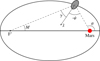 |
Fig. 1 Librational geometry, where θ and M are the true and mean anomalies of Phobos in its orbit, ψ is the tidal libration angle, γ is the physical libration angle, and F′ represents the empty focus of the ellipse. The angle between the moon-to-empty-focus and the apse lines is equal to M up to O(e2) (Murray & Dermott 1999). The eccentricity of this figure has been greatly exaggerated for visualization purposes. |
2.2 Kinematic rotation descriptions
There is a number of ways to kinematically parameterize the orientation of a body (Fukushima 2012). For Solar System bodies, the most popular manner is by specifying the orientation of the rotation axis – or pole – by its right ascension and declination with respect to a frame of inertial orientation, together with the longitude of the meridian in said frame (see e.g., Archinal et al. 2018; Burmeister et al. 2018). Various closed-form expressions have been developed for their evolution in time, for a range of bodies (Duxbury & Callahan 1981; Stark et al. 2017; Archinal et al. 2018).
Phobos’s pole follows the long-term orientation of the orbital plane normal (Stark et al. 2017), and Phobos rotates about it at a frequency that follows the long-term evolution of the mean motion (Jacobson et al. 2018). For the typical Phobos-fixed frame (see Sect. 2.1), this means that, averaged over time, Mars’ Phobos-fixed position is constant at a latitude and longitude of 0. Superimposed on this constant value is a long series of oscillatory variations known as librations. When limiting this phenomenon to two dimensions, we have the situation represented in Fig. 1. The deviation of Phobos’s body-fixed x-axis (corresponding to its long axis) from the moon-planet direction is sometimes termed the tidal libration angle (Lainey et al. 2019), and is denoted ψ in Fig. 1. It is related to the longitude of Mars in Phobos’s body-frame λ as
 (10)
(10)
For a tidally locked satellite with constant rotation rate in an unperturbed eccentric orbit, it can be shown that the satellite’s long axis approximately points toward the empty focus of the orbital ellipse (to order e2) (Murray & Dermott 1999). This is a purely geometric effect entirely determined by the satellite’s eccentricity, and commonly referred to as the optical libration (denoted by φ). In addition, the response of the satellite’s rotation to forcings induces the so-called physical librations, represented by the angle γ in Fig. 1. These physical librations are not only influenced by orbital characteristics, but also by the moon’s inertia tensor, and hence its interior properties. The total libration angle ψ is given by the combined effect of optical and physical librations, where the former can be expressed as (see Fig. 1)2
 (11)
(11)
which is accurate to O(e2). Using the empty focus as reference direction with respect to which we compute librations is potentially advantageous, since we know that the librations around this reference direction will be zero in the absence of torques or orbital perturbation. If one would instead use the vector to the planet as reference direction, we must still consider the nonzero optical libration in Eq. (11), even in the absence of any forcing (when γ = 0).
The use of the empty focus as reference direction does, however, present a complication related to its implementation in a numerical model. Because Phobos’s orbit is not perfectly Keplerian, the location of the empty focus is not constant, but instead adjusts itself according to variations in the orbit’s osculating elements. Therefore, if we assume that the long axis of the body would always point to the instantaneous empty focus of the osculating orbit, we would be assuming that the rotation of the satellite instantaneously responds to orbital perturbations, which is not true over short timescales (see Sect. 2.3).
Regardless of the choice of reference direction for the computation of the longitudinal rotation angle, we require a model to compute the physical libration angle γ as a function of time. The period at which the longitudinal libration undergoes the strongest forcing is the once-per-orbit one, by virtue of Eq. (11). Consequently, γ is typically given by Eq. (12) where 𝓐 is just the amplitude of the once-per-orbit oscillation – the so-called libration amplitude. The scaled libration amplitude ℬ can also be used (Lainey et al. 2019), for which we have
 (12a)
(12a)
 (12b)
(12b)
The relation between the two libration amplitudes then directly follows from
 (13)
(13)
The value of the physical libration amplitude provides information on Phobos’s moment of inertia through Eq. (14) (Murray & Dermott 1999), where σ = (B − A)/C and A ≤ B ≤ C are Phobos’s main moments of inertia. Thus, estimation of the once-per-orbit libration amplitude can help constrain the interior structure of Phobos, since for rigid bodies we have
 (14a)
(14a)
 (14b)
(14b)
In our implementation, we follow the model by Lainey et al. (2019), using ℬ as free parameter. By using the following equations:
 (15a)
(15a)
 (15b)
(15b)
which are valid to O(e2), we can compute the angle ψ directly. This offers a very convenient implementation, which is therefore widely used when modeling the dynamics of natural satellites (e.g., Lainey et al. 2019; Fayolle et al. 2023). However, the use of this model leads to the implicit use of the instantaneous location of the empty focus. This implies that the rotation would follow the orbit on both short and long time-scales, which results in minor mismodeling of the rotation (as discussed above). This is very well illustrated in Fig. 2, where the frequency content of the once-per-orbit longitudinal tidal libration ψ has been plotted together with the frequency content of the mean motion. As can be seen, the frequency content of ψ has a main peak at the average mean motion, and also smaller peaks at other frequencies, corresponding to the frequencies at which the osculating mean motion n varies – the largest of them occurring at integer multiples of the average mean motion. This shows that, by using Eq. (15) for the once-per-orbit libration, we are introducing a series of additional librations, as undesired artifacts of our model choice (and the spurious assumption that the rotation will follow the osculating orbit on short timescales). The largest of these “unintentional” additional librations occurs at the 2n frequency, and has an amplitude that is around 0.01 degrees (or about 1% of the once-per-orbit libration). On the other hand, the coupled approach, by automatically ensuring the complete consistency of the satellite’s translational and rotational dynamics, is immune to such issues. Although the discussion has focused on longitudinal librations – oscillations about Phobos’s z-axis – and the orientation of Phobos’s x-axis in the orbital plane, because those are indeed the most prominent aspects of Phobos rotational motion, other oscillations exist about Phobos’s x and y axes, called wobble and latitudinal librations respectively. Kinematic descriptions of the rotation of Phobos usually don’t include them, and they have rarely been considered in Phobos’s dynamics, with Borderies (1977) and Rambaux et al. (2012) being works that were partly dedicated to the study of latitudinal librations. In our kinematic model, and in agreement with the most typical representation of natural satellites’ rotations, we assume that Phobos’s equator follows the instantaneous orbital plane, removing any freedom for these types of librations. Nevertheless, an extended kinematic model for Phobos’s rotation could also include these terms.
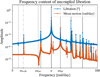 |
Fig. 2 Frequency content of the tidal longitudinal libration of an uncoupled translational state in which a fully locked configuration of Phobos has been assumed, together with a once-per-orbit longitudinal libration. |
2.3 Normal modes and damping
The rotational equations of motion (Eq. (9b)) can be linearized for small angles ε around each axis of the Phobos-fixed frame. This yields Eq. (16a) for the evolution of the (small) longitudinal libration angle (Rambaux et al. 2010) and an equivalent but coupled system for the other two angles (see e.g., Borderies & Yoder 1990). Here, f is the appropriate component of the torque – the forcing. In the homogeneous case (for f = 0), this equations still yields an oscillatory solution, with a frequency of oscillation ωo. This oscillation is called the rotational normal mode, and there exists one for each axis of the Phobos-fixed frame. These normal modes are physical properties of the body itself:
 (16a)
(16a)
 (16b)
(16b)
In the general case where f ≠ 0, oscillations appear at an infinite range of frequencies. In the context of moons – and more specifically Phobos – these oscillations excited by forcings are called forced librations. These forced librations about each axis are given, in the linearized case, by the solution to Eq. (16a), namely Eq. (16b) (Rambaux et al. 2010), where fi and ωi are the amplitudes and frequencies of all the components that make up the forcing f. It is important to note that components of the forcing with a frequency close to the normal mode produce a strong librational response. For Phobos, its longitudinal normal mode is close to the orbital mean motion, the frequency at which the forcing is strongest. As a result, forcings are expected close to the normal modes which, even if weak, still produce a relatively strong response.
Analytical expressions for the frequencies of the normal modes are (Rambaux et al. 2012):
 (17a)
(17a)
 (17b)
(17b)
 (17c)
(17c)
 (17d)
(17d)
 (17e)
(17e)
where ωlon, ωlat, and ωwob are the longitudinal, latitudinal, and wobble normal mode frequencies (about Phobos’s z-, y-, and x-axes, respectively) and A ≤ B ≤ C are Phobos’s main moments of inertia. Following the analysis of Rambaux et al. (2012) for Phobos, we provide the latitude libration frequency in the inertial frame rather than the Phobos-fixed frame, where its frequency is decreased by n (Rambaux & Williams 2011). Since our work is aimed at modeling the coupled orbital-rotational dynamics in inertial space, this choice is the most suitable one for our work.
In practice, the response at the normal mode itself (first right-hand side term in Eq. (16b)) has typically been damped by dissipative effects over long timescales. The normal modes can thus technically be removed from the rotational response. However, when Eq. (16a) is integrated – and more generally Eq. (9b) – both the normal modes and the forced response generally arise as part of the numerical solution. Unless a physically realistic initial state is used, one needs to forcefully remove the normal modes from the solution.
For most bodies, the forcing frequencies are far enough from the normal modes that free librations are easily identifiable in a Fourier decomposition after integration of the rotational equations of motion (Eq. (9b)). In those cases, damping the free modes can be achieved by the removal of the free librations in frequency space. In the case of Phobos, normal mode frequencies are very close to a range of forcing frequencies, making it very difficult to distinguish the free modes from the forced librations, and an alternative needs to be considered. In this work, we do this in the same way as Rambaux et al. (2012), which is to introduce a damping algorithm, making use of a virtual torque in the equations of motion. This virtual torque is computed as to preserve the average rotation of Phobos around its z-axis while opposing any other rotation. The dynamics are propagated forward in time with the torque, and the final state is used to propagate the dynamics backward without the torque. This procedure is performed several times in an iterative process to generate the initial state used to propagate Phobos’s dynamics. Specific details on this algorithm and the computation of such a torque can be found in Appendix B.
2.4 Coupled and uncoupled models
In order to study the couplings between Phobos’s translational and rotational dynamics, and the limitations of the classical uncoupled model, the equations of motion (Eq. (18)) were integrated both in a coupled manner and an uncoupled manner – from now on termed the coupled model and the uncoupled model respectively. For the coupled model, the state derivatives of the translational and rotational state vectors from Eq. (9) can be written explicitly as
 (18a)
(18a)
 (18b)
(18b)
clearly indicating that Phobos’s dynamics are dynamically coupled by nature. However, an uncoupled model can be defined that propagates only the translational equations of motion (Eq. (18a)) by imposing some fixed xr(t) that is not integrated. In such a case, which we term the uncoupled model, we have
 (19a)
(19a)
 (19b)
(19b)
turning the computation of xr into an algebraic equation that depends on the current xt rather than a differential equation. The implementation of this algebraic relation for the case of Phobos is defined in terms of one or more librations, and is described in more detail in Sect. 2.2. In a few instances discussed in this paper, an additional model becomes useful that features Phobos in a fully locked configuration with respect to Mars (fully locked model). This is to say that Phobos’s long axis is forcefully aligned with the moon-planet direction at all times.
The typical implementation of ɡr in the determination of ephemerides, which is also the one we use here, features only a once-per-orbit longitudinal libration. Following Eq. (19b), the rotational state xr of Phobos is not driven anymore by torques, but rather is completely determined by the translational state xt and some extra parameters, namely 𝓐 or ℬ (where we chose to use the latter as free parameter in our models). We discuss the disadvantages of uncoupled models, and detailed rationale for our choice of a coupled model, in the next section.
In the coupled model, we used an initial state for which the free mode is damped using the damping algorithm discussed in Sect. 2.3. For consistency, we used the same initial translational state in our coupled and uncoupled models. In the uncoupled model, we imposed xr such that Phobos was in a fully locked configuration (its long axis always pointing directly toward Mars), upon which a once-per-orbit tidal longitudinal libration of amplitude ℬe was superimposed. This angle was computed as in Eq. (12b), the factor e sin M computed as in Eq. (15a). We chose the value of ℬ that best reproduces the once-per-orbit longitudinal libration that was obtained from the coupled model. To obtain this value, we performed a Fourier transform of Phobos’s tidal longitudinal librations as computed by the coupled model, from which we determined the value of ℬe.
Finally, it should be understood that the role of librations in the two models is entirely different. For the uncoupled model, the libration amplitude (or, when using such an approach as Le Maistre et al. (2013) or Dirkx et al. (2014), a list of libration amplitudes and phases) is an input to the model, and a free parameter that can be estimated. For the coupled model, the librations are an output of the model: in evaluating the coupled equations of motion, the concept of librations plays no role (see Eq. (9)). It is then only in the post-processing and analysis ofthe results that librations become relevant (Rambaux et al. 2012).
2.5 Limitations of uncoupled models
The uncoupled model we used in this study, as well as by e.g., Lainey et al. (2019), presents two limitations when applied to high-accuracy applications that will be required in the future:
The first limitation is the simplification of the parametrization of the rotational motion, which is reduced to a single longitudinal libration at the orbital frequency.
The second limitation is the use of Eq. (15) to compute this single longitudinal libration angle, which slightly misrepresents the exact behavior that is to be modeled.
Here, we discuss these two issues in detail and argue why the use of a coupled model, rather than a more detailed multilibrational model, is a preferred solution for sustainable and practical high-accuracy ephemeris determination.
The first limitation could be mitigated by expanding the librational spectrum included in the satellite’s rotational model, as done by Chapront-Touze (1990). However, this requires an a priori knowledge of the relevant librational frequencies. Le Maistre et al. (2013) and Dirkx et al. (2014) chose the relevant frequencies reported by the numerical integration of Rambaux et al. (2012). However, these are particular to a given forcing spectrum as defined by its orbit (Lainey et al. 2007) and a given inertia tensor, as defined by its interior model (Willner et al. 2010). The latter point in particular limits the degree to which a valid spectrum can be determined before an ephemeris determination, since the relevant libration frequencies depend on the frequencies of the normal modes. These frequencies in turn depend on the moments of inertia, which are typically one of the parameters that can be estimated during an ephemeris determination. This presents a challenge, since the ephemeris determination requires the set of relevant libration frequencies to have been established, but knowing which set of frequencies are valid requires improved knowledge of the moments of inertia, which is one of the outputs of the ephemeris determination. Such circular logic is particularly important for Phobos, where the frequency of the proper mode ω0 is close to the forcing frequencies, and a slight shift in the former can have a strong impact on which forcing terms lead to a relevant response (see Eq. (16b)). Resolving this for an uncoupled model would require an iterative approach, where the set of frequencies that is considered is redetermined after an adjustment of the interior properties during the estimation of the ephemeris. In a coupled model this dependency of the response on the interior is automatically captured without any a priori tuning (Dirkx et al. 2019).
In addition to complications in the selection of relevant frequencies in a multilibrational model, applications with tighter fidelity requirements in dynamical and observation model would necessitate the use of models with a large number of librations (Le Maistre et al. 2013; Dirkx et al. 2014), resulting in a large number of free parameters to adjust in the data inversion, and large correlations between them. This is an artifact of the large number of free parameters, and not an issue for a coupled model (Dirkx et al. 2019). This problem can be resolved by introducing suitable interrelations between the libration terms (Borderies & Yoder 1990), at the cost of significant model tuning.
The second limitation stems from the fact that our libration model was parameterized by the mean anomaly rather than being an explicit function of time. A model that is an explicit function of time is typical in high-accuracy uncoupled rotation models of e.g., Earth (Petit et al. 2010) or Mars (Le Maistre et al. 2023; Goli et al. 2024). Using such a model for the rotation of a tidally locked body during a computation of its orbital dynamics is not as straightforward, due to the requirement that spin-orbit resonance is to be maintained. In a coupled model this is enforced dynamically, but in an uncoupled model a change in the translational dynamics must result in a suitable adaptation of the rotational state to enforce this resonance. The reason that this must be strictly enforced is due to the extreme sensitivity of the spherical harmonic acceleration, the gradient of Eq. (3b), to small constant shifts in the longitude angle λ. Specifically, even a small bias in this angle will result in a small but constant along-track acceleration, resulting in a linear drift in mean motion, a quadratic drift in along-track position, and a divergence of the real and modeled orbit. This effect is equivalent to that of a nonzero S22 (and tidal dissipation in the planet or moon) in the situation where the long axis points to the empty focus (Fayolle 2025).
In our model, we enforced consistency between orbit and rotation by using Eq. (15) to compute the longitudinal libration angle ψ. Although this ensures that the two always remain in phase, it introduces spurious librational frequencies by implicitly using the osculating mean motion n (Fig. 2). The amplitude of these spurious oscillations reaches up to 0.01 degrees, which is the same order of magnitude as the largest of the additional (e.g., other than once-per-orbit) libration terms. Consequently, even if we were to add additional libration terms in the model, our ability to accurately represent the resulting time evolution of Phobos’s orientation in space would not improve meaningfully, unless an alternative to Eq. (15) is used to ensure orbital-rotational consistency. However, ensuring such consistency within a single propagation is not possible, since one must impose an evolution of the rotation pole and rotation rate that follows the long-term trend in the orbital evolution. During an orbital propagation, one cannot readily disentangle the behavior due to short-periodic variations from the longer-term variations and trends in the orbit.
Rather than developing and applying an uncoupled model and associated estimation strategy that overcomes these problems, we argue that – at the accuracy levels where it becomes relevant (around 0.01 degrees for Phobos) – it is preferable to move to a dynamic representation of the rotation. Such a method does not suffer from these issues, while at the same time ensures that an estimation of the coupled orbital-rotational dynamics consistently captures the impact of the degree-two gravity field coefficients on the orbital dynamics and (through the relation of these terms to the inertia tensor) the rotational dynamics (Dirkx et al. 2019).
The use of a dynamic model for coupled orbital-rotational motion has also been adopted for the Moon. Due to the avail-ability of LLR data, high-accuracy lunar libration models are required. As described by Newhall et al. (1983), the use of an uncoupled rotation model for the Moon led to issues from “the use of an analytical theory for the computation of lunar libration, acting as a forcing function for the system through figure perturbations”. It must be stressed that this does not preclude the use of uncoupled models. An analysis of LLR data based on kinematic models is presented by Chapront et al. (1999b), who used the model by Chapront et al. (1999a) for their fit, an analytical model complemented with fits to numerical integrations. They showed that this can adequately fit the data, but at the expense of a complex specific model tailored to one body. This brief case study of the Moon reinforces our argumentation above: while it is indeed possible to develop an uncoupled model with the required level of accuracy, doing so requires significant body-specific model development. We stress that explicit models as a function of time with (many) more terms than only the once-per-orbit libration (Chapront-Touze 1990; Stark et al. 2017; Jacobson et al. 2018) are eminently useful in many other applications that require a high-accuracy Phobos reference frames. It is only for the computation of orbital dynamics that the strict consistency requirement between orbit and rotation makes their direct application challenging.
An overview of historical dynamical model development for the case of Phobos was given by Jacobson & Lainey (2014). There, the shift from analytical to numerical models for Phobos’s orbit was well described. One of the main drivers toward a numerical formulation was stated to be the difficulty of fitting new observations to the analytical model, since this requires a recomputation of the underlying numerical model (to which the analytical model is fitted). This is in line with our discussion above, where retaining an uncoupled model at higher accuracy requires iterating the orbital model to re-enforce the consistency between orbital and rotational motion.
3 Estimation
In our analysis, we first quantify the difference between the coupled and uncoupled model when using the exact same model parameters – initial state, libration amplitude and gravity field. However, in quantifying how valid it is to use an uncoupled model in place of a coupled model, it is required to investigate the extent to which the uncoupled model is able to approximate the orbital dynamics of the coupled model, and look at what differences still remain. We performed such an analysis by means of estimations. This section explains our estimation methodology and the rationale in the context of the problem at hand.
We first define our general estimation method in Sect. 3.1. We then discuss the advantages of using a coupled model instead of the classical uncoupled formulation in Sect. 3.2, focusing on the implications for the estimation process and results. Finally, the two main elements of the estimation are presented, i.e., the observations (and observation model) and the estimated parameters (and estimation model), in Sect. 3.3.
3.1 The estimation problem
Provided a set of observations z either obtained from reality or generated with a simulation model, a set of differential equations – hereafter the “estimation model” – can be used to replicate them, providing the so-called model values h. The governing equations in this estimation model contain a number of free parameters, collected in a vector y that determines the value of h, so that h = h(y) (for the type of applications under consideration here, y typically includes one or more initial states, and physical parameters that influence the dynamics). The estimation can be understood as the process of finding a vector y* such that the differences between z and h, called residuals and defined as in Eq. (20a), are minimized in the least squares sense: i.e., the quantity ε Tε is minimal. The estimator is the method by which the estimation is performed. In this work, a linearized least squares estimator is used.
To compute y*, the model values are linearized around a reference ho = h(yo) and one can approximate the residuals as in Eq. (20b), where H = ∂h (yo) /∂y (usually called the design matrix) and ∆y = y − yo.
 (20a)
(20a)
 (20b)
(20b)
Then, an iterative process begins, each iteration consisting of computing  and updating the reference to
  . This new reference is used to linearize hi+1 in the next iteration. The parameter update
  is computed by solving the so-called normal equations in Eq. (21).
 (21)
(21)
In this work, we consider the estimation to be converged if the residuals and parameter estimate are stable for several iterations.
3.2 Influence of the uncoupled model’s limitations
Consider a set of parameters yb (e.g., the initial state xo) with which the coupled model has been propagated. Using these parameters, the coupled model produces a state history xc(t, yb). If an estimation is performed in which the observations, e.g., Cartesian positions, are taken from xc(t, yb) and then an uncoupled model is used as estimation model (see Fig. 3), the vector of residuals can be written as in Eq. (22), where ru(t, y) is the model values produced by the uncoupled model when the set y of parameters is used. Note that, because the differential equations that generate xc and xu are different by definition, ε(t, yb) is not nil and the solution to the corresponding least squares problem is some nonzero vector y* = yb + ∆y* ≠ yb.
Replacing h = ru(t, y) and z = rc(t, yb) in Eq. (20), the residual vector can be rewritten as
 (22)
(22)
In this equation, ru and rc denote the Cartesian position of Phobos, as extracted from the solution history for the uncoupled and coupled dynamical model, respectively (Fig. 3). The parameter increment ∆y* appears in order to account for the differences in r(t) generated by differences between the coupled and uncoupled models. In other words, the effect that the limitations of the uncoupled formulation have on the trajectory is absorbed by this ∆y*. This absorption is such that the residuals are minimized, and although ε(t, y*)T ε(t, y*) is indeed smaller than ε(t, yb)T ε(t, yb), it is never 0. Absorption is then said to be imperfect and some residuals are left, representing a part of the effects that could not be absorbed by any of the parameters.
However, absorption can lead to misleading results. Absorbing the mismodeled rotation signatures (either caused by couplings or artificially introduced by the uncoupled model implementation, see Eq. (15)) into the parameters contaminates the solution and makes it differ from the true yb. This is the scenario in current state-of-the-art estimations. Phobos’s real life dynamics incorporate, by definition, all possible couplings, while state-of-the-art estimation models are uncoupled. In trying to estimate the values of yb through estimation, a solution y* is instead obtained, which contains the bias ∆y*, while yb remains unknown. One aim of this work is to quantify this bias ∆y*. The parameter vector y often includes the once-per-orbit longitudinal libration angle or Phobos’s gravity coefficients C20 and C2,2, all of these containing information about Phobos’s interior. Mis-estimation of these parameters effectively results in misinformation about the interior structure of Phobos.
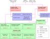 |
Fig. 3 Schematic of the work done in this paper. |
3.3 Estimation settings
We performed estimations using the uncoupled model as estimation model and the coupled model as truth model. This setup is an idealized representation of the current state-of-the-art in ephemerides generation, where the “truth model” (physical reality) is described by a coupled model, but the “estimation model,” used by e.g., Lainey et al. (2007); Jacobson (2010); Jacobson & Lainey (2014); Lainey et al. (2021) uses an uncoupled model. By taking this approach (illustrated in Fig. 3), we can isolate and analyze the influence of the present-day approach of using an uncoupled rotational model for Phobos.
This work uses simulated observations z in all the performed estimations, which have been generated using the coupled model. We note that this approach is in contrast to a seemingly similar analysis by Yang et al. (2024), who simulate observations from the real ephemeris (uncoupled model) and fit these to a coupled model using the approach described in more detail by Mazarico et al. (2017) and Dirkx et al. (2019). We discuss the distinction between the two approaches in Sect. 5. Our observations consist of position observables. This means that the word “observation” in this work is to be understood as a position vector, more specifically the position vector of Phobos with respect to Mars, with the components expressed in the J2000 reference frame (see Sect. 2.1), as produced by numerical integration of the coupled translational-rotational equations of motion. These observations were generated every 20 minutes, starting (arbitrarily) one Julian year after the epoch J2000. Observations are assumed noiseless and ideal.
The residuals of our estimation represent the remaining dynamical behavior of the coupled model that the uncoupled model is not able to mimic in any way. As explained in Sect. 3.2, estimated parameters are mis-estimated in the process, since they absorb part of the effect of this coupling. Our simulation results quantify this effect directly. Four different estimation sets were performed, estimating different parameters each. These sets estimate:
Set 1: initial translational state, xt,o
Set 2: initial translational state, xt,o, and once-per-orbit longitudinal libration amplitude, ℬ (like Jacobson 2010 or Lainey et al. 2021)
Set 3: initial translational state and Phobos’s (normalized) degree 2 zonal gravity coefficient, xt,o and
 .
.Set 4: initial translational state and Phobos’s (normalized) degree 2 sectorial gravity coefficient, xt,o and
 .
.
The first set provides a baseline as to how well the uncoupled model can emulate the coupled model when the rest of the parameters are the same. Comparisons of other estimations with this one quantify how well other dynamical parameters can absorb the effects of couplings. The other sets represent variations on typical ephemeris estimation schemes of Phobos in which a physical property is estimated along with the ephemerides. We note that the estimation of more than one of these quantities from the ephemerides leads to a near-ill-posedness in the solution, since each has a comparable impact on the orbit: primarily a linear rate in the longitude of periapsis ϖ(= ω + Ω), (specifically Jacobson 2010):
 (23)
(23)
Results of estimation sets 2–4 quantify how well an uncoupled model can emulate a coupled model – for which residuals have to be studied – and how much the estimated parameters are contaminated by the dynamical mismatch of couplings.
4 Results
This section presents the results we obtained from our simulations, which we categorize into three groups: state propagation (Sect. 4.1), rotation (Sect. 4.1.2), and parameter estimation (Sect. 4.2). For the state propagation, the effect of couplings was analyzed by using an identical initial translational state and, for the uncoupled model, a once-per-orbit libration amplitude that is identical to that which is obtained from the coupled model (Sect. 2.4). How couplings impact the results of estimations was studied through the analysis explained in Sect. 3.2. A flowchart summarizing the full procedure followed in this work is provided in Fig. 3.
In the remainder of the text, extensive use is made of the so-called RSW frame. At any point of a trajectory, one can define a reference frame formed by the right-handed triad  . Unitary vectors
  and
and  are parallel to the instantaneous position and orbital angular momentum vectors, while ŝ (which, due to the near-circularity of the orbit, is close to the velocity unit vector) completes the triad. The RS plane corresponds to the plane of the instantaneous elliptical orbit (in-plane), while the W direction is the direction perpendicular to it (out-of-plane).
4.1 State propagation
As a first approach to the study of couplings, the same initial state was propagated using the coupled and uncoupled models for a total of 81 920 hours (around 9 years and 4 months). Proper damping of the normal modes (see Sect. 2.3 and Appendix B) requires long damping times. The selected propagation time was the longest that the equipment used could hold in memory. There are two main areas in which the differences between these two simulation results were analyzed: translation and rotation.
4.1.1 Translation
The difference in the state propagation using the coupled and uncoupled model are shown in Fig. 4. Here, Fig. 4a provides a direct order-of-magnitude context, showing that the norm of position differences between the coupled and uncoupled trajectories accumulate to about ~40 m after about 10 years. Here, we reiterate the fact that the libration amplitude in the uncoupled model was set to a value extracted from a Fourier transform of the results of the coupled model. Consequently, the impact of once-per-orbit longitudinal librations will be (to first order) the same for the coupled and uncoupled model. Differences between the two, on the other hand, originate from neglected libration components and couplings in the uncoupled case, as well as implementation considerations, as underlined in Sect. 2.4.
The time behavior of all three components of the propagation difference can be seen in Fig. 4b. The along-track component shows a secular trend (the uncoupled trajectory gets ahead of the coupled one) superimposed by oscillations of ever-increasing amplitude. The radial and out-of-plane components do not show a secular component, and only oscillate around ~0 m with a growing amplitude of up to 4 m at the end of the integration time. The largest of these oscillations occurs at the orbital frequency, as seen in Fig. 4c. Oscillations in the order of millimeters are present at frequencies very close to the latitudinal normal mode (ωlat = 27.165 rad/day), a frequency close to which Rambaux et al. (2012) identified a resonant forcing. They noted that these frequencies are due to oscillations in Phobos’s inclination and changes in the secular part of the mean anomaly, and the fact that there exist differences at this frequency between the coupled and uncoupled model indicates that this libration has a noticeable influence on the orbit that, although small, cannot be accounted for by uncoupled rotational models.
It is also interesting to note the presence of peaks at multiples of the orbital frequency (2n and 3n specifically) in Fig. 4c. These are indeed not to be automatically ascribed to couplings, but also result (at least in part) from artificial signatures introduced by the traditional implementation of the uncoupled model, which defines the satellite’s orientation based on its instantaneous orbit (Eq. (15), see discussion in Sect. 2.2). This inherent limitation of the classical uncoupled implementation, which oftentimes remains overlooked, is naturally avoided in the fully consistent translational-rotational solution provided by the coupled approach.
The main differences in position are seen to be a secular trend in along-track position and the onset of radial and out-of-plane oscillations (Fig. 4b). We can see in Fig. 4d that the difference in orbital inclination of the coupled and uncoupled solution does not have a short-periodic component. Instead, the dominant frequency of the inclination is 0.01 rad/day, driving the low-frequency oscillations in the RSW components of the effects of couplings, as mentioned above. The notable along-track difference demonstrates that including a single once-per-orbit libration, as done in classical uncoupled formulations, cannot fully account for Phobos’s longitudinal rotational motion. This implies that the limitations of the uncoupled model are not limited to the omission of latitudinal components, but also have a noticeable in-plane effect. The secular along-track trend in Fig. 4b nonetheless indicates that couplings induce comparable signatures on the in-plane motion as the once per-orbit libration, since all longitudinal librations – once-per-orbit or otherwise – are bundled together in Mars’ Phobos-fixed longitude in the evaluation of Phobos’s gravitational potential (Eq. (3)). This is reinforced by a comparison between the effects of couplings and the effects of the once-per-orbit longitudinal libration. Figure 5 shows in red the effect of the once-per-orbit libration on the orbit, indicated by the differences between the uncoupled model and the fully locked model. In particular, Fig. 5a shows that both couplings and the libration have qualitatively similar in-plane effects. The out of plane effects (Fig. 5b), however, are completely different. In the context of parameter estimation, this points at the once-per-orbit libration amplitude having a lot of potential in absorbing the effects of couplings, which means that it will likely be mis-estimated in minimizing the in-plane components of the residuals generated by couplings (see Sect. 3).
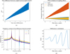 |
Fig. 4 Propagation results. The differences in position is studied in different ways: norm (panel a), components (panel b), frequency content (panel c) and Keplerian elements (panel d). Vertical lines in the bottom left picture represent (multiples of) the mean motion (n) and latitudinal normal mode (ωlat). Here, the coupled states have been subtracted from the uncoupled ones. Panel a: norm of position difference between the states propagated by the uncoupled model and those propagated by the coupled model. Panel b: time evolution of the RSW components of the position differences between the coupled and uncoupled trajectories. Panel c: frequency content of the RSW components of the position differences between the coupled and uncoupled trajectories. Panel d: differences in inclination between the coupled and uncoupled trajectories. |
4.1.2 Rotation
Differences in rotational motion can be divided in two axes: longitudinal and latitudinal differences. The uncoupled model, by definition, produces no latitudinal librations because Phobos’s orbital and equatorial planes are always coincident (see Sect. 2.2). It is still of interest to study the latitudinal librations produced by the coupled model (see Sect. 2.4). Table 1 collects the largest peaks of the frequency spectrum of the tidal latitudinal librations, i.e., Mars’ Phobos-fixed latitude. In studying these types of librations instead of the physical librations, the low-frequency orbit-induced effects are removed. In these lines, tidal latitudinal librations are purely associated with high-frequency forcings, which are amplified if they are close to Phobos’s normal modes. It is to be noted that the first two components in Table 1 correspond to the second and fifth terms tabulated by Rambaux et al. (2012), associated with different combinations of the Delaunay arguments and consequence of a forcing occurring at that frequency3. These forcing frequencies are close to the latitudinal and wobble normal modes (ωlat = 27.165 rad/day, ωwob = 7.336 rad/day), producing an amplified libration when integrating the rotational equations of motion. The third term in Table 1 occurs at the orbital frequency of the mean motion, while the fourth corresponds to a forcing close to the longitudinal normal mode (ωlon = 12.354 rad/day). On the other hand, longitudinal librations are present in both the coupled and uncoupled models. The largest terms resulting from the coupled model are provided in Table 2. As a point of reference, the first and second peaks can be correlated to the second and fifth terms in Table 4 by Rambaux et al. (2012). The results for the uncoupled model are tabulated in Table 3, which corresponds to Fig. 2. As a reminder, the uncoupled model should ideally only contain one single libration at the orbital frequency. However, this is not the case due to the use of Eq. (15b). Therefore, all additional frequencies present in the uncoupled libration spectrum are not physical, but artificial effects of the commonly adopted implementation strategy. On the other hand, the results of the coupled model account for the full forcing spectrum and provide a realistic and self-consistent mapping from forcing to response, including weak forcing terms at frequencies close to the normal modes (see Sect. 2.3) which are amplified by this proximity.
The once-per-orbit libration amplitude should be the same in both models – as explained in Sect. 2.4. Phobos’s once-per-orbit longitudinal libration amplitude can be extracted from the results of the coupled model, producing a scaled tidal libration amplitude of ℬ = 3.29918 (a physical libration amplitude of 𝓐 = 1.12412°, the one used for the uncoupled model in this work), which can be compared to the analytical prediction of Eq. (14), i.e., ℬ = 3.29807 rad. The difference between the two values is of 0.03%, which translates in an error of 10−3 degrees in the amplitude of the once-per-orbit physical libration amplitude. Note that the analytical prediction was developed in the context of uncoupled models, and their predictions matching so well with the result of a coupled propagation indicates that uncoupled models can naturally replicate the once-per-orbit libration amplitude of the complex coupled dynamics of Phobos.
The origin of librations in the coupled and uncoupled models is very different. The uncoupled model, through the implicit use of osculating orbital elements in computing the libration angle through Eq. (15), shows longitudinal librations at the frequencies at which accelerations naturally occur. In the coupled model, torques are expected to naturally occur, to a large extent, at similar frequencies as the accelerations. Their effect on rotation is approximately given by Eq. (16b). Thus, in the coupled model, the normal modes play a big role in Phobos’s rotational response: torques that occur close to the normal modes (ωi ≈ ωo) give rise to large-amplitude forced librations compared to the amplitude of the forcing. An illustrative example is that of the longitudinal libration occurring near ~27.15 rad/day (Table 2). This frequency is around twice the synodic frequency between Phobos’s orbit and the Martian rotation, and very close to the latitudinal normal mode. Therefore, this leads to a relatively strong response in the coupled model. We see a response at an identical frequency in Table 3 for the uncoupled model. However, the origin of this response is very different: it is the result of the use of Eq. (15b) in which fast oscillations in the empty focus are erroneously mapped to longitudinal librations. Rather than providing any physical information on its rotation, these results indicate the limitation of using this particular libration model for Phobos (Sect. 5.1).
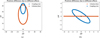 |
Fig. 5 Comparison of the position differences between the coupled and uncoupled trajectories (blue) and the position differences between the classical uncoupled model (i.e., with once-per-orbit libration) and fully locked (i.e., no libration) trajectories (orange). Only the final ten orbits of the nine years and four months have been plotted. Note the different units. Panel a: in-plane projection of position differences. Panel b: out-oſ-plane projection of position differences. |
Strongest components of latitudinal tidal librations from the coupled model.
Strongest components of longitudinal tidal librations from the coupled model.
Main peaks of the tidal longitudinal libration as computed by the uncoupled model.
4.2 Parameter estimation
In this section, we present the results from the setup described in Sect. 3. We simulated observations from a coupled model, and then estimated the dynamics using an uncoupled model. This allowed us to quantify how much of the difference between a coupled and uncoupled propagation (Sect. 4.1) can be absorbed by adjusting parameters of the uncoupled model. The remaining effects that cannot be absorbed are observed as estimation post-fit residuals.
We outline the simulations we ran in Sect. 3.3, which were performed for different arc lengths up to 1000 days (the maximum that the equipment allowed). In assessing the quality of the estimation, the residuals and estimated parameter difference from truth were used as figures of merit. The former were studied both as norms and as RSW components.
4.2.1 Estimation of initial state
First, an estimation of initial state only was performed with the uncoupled model, using observations generated by the coupled model. In this estimation, focus was put on an analysis of residuals. These residuals provide insight on what effects the initial state cannot absorb and represent an upper bound for residuals of later estimations. Residuals that remain in later estimations represent effects that additional parameters cannot absorb, while reduction in residuals represent effects of couplings that additional parameters can absorb.
Mismodeling in the uncoupled case could be seen to impact the along-track motion in a more significant way than the R or W components when comparing the propagation of coupled and uncoupled dynamics (see Sect. 4.1).
Figure 6a shows how fitting the initial state reduces the differences between the coupled and uncoupled models, in terms of the norm of the position differences between the two. It shows that differences are reduced by a whole order of magnitude, from a maximum of around 15 m to below 2 m. Recalling Eq. (22), the blue line corresponds to |ε(t, yo)| while the red line corresponds to |ε(t, y*)|. As expected, the norm of the residuals – red curve in Fig. 6a – reaches a minimum near the center of the arc, and increases to reach a maximum at the two ends of the arc. The difference between the true and estimated orbits are decomposed into RSW components in Fig. 6b. The S component is again the largest component of the residuals, reaching 1.5 m at the ends of the arc, while the W component is the smallest one and reaches maxima of around 0.5 m. A Fourier decomposition of all three components can be seen in Fig. 6c. Indeed, the dominant frequency is that of the mean motion n, with contributions at millimeter level of twice the mean motion and half the frequency of the latitudinal normal mode. Furthermore, there are also a series of peaks at sub-mm level that, although likely below the noise floor of near-future observation techniques, can all be correlated to frequencies close to the normal modes, at which weak forcings are amplified by resonance and significant librations were observed. The slow frequencies of the residuals components have been cropped out of Fig. 6c for clarity, but they all show large oscillations below 0.1 rad/day and at around 0.01 rad/day, coincident with the long term orbit-induced effects mentioned in Sect. 4.1.
As a specific example of the impact of the fitting on the orbital geometry, the inclination difference between the coupled and uncoupled propagation is indeed reduced by the estimation (Fig. 6d), but a long-periodic behavior remains. Moreover, a frequency decomposition revealed that both the pre-fit and post-fit inclination residuals contained a significant peak close to the wobble normal mode, owing again to the inability of an uncoupled model to emulate the resonance properties of the rotational equations of motion.
For the sake of generalization, it is useful to see how our results would extrapolate to estimations performed over arcs of different lengths. To this end, Fig. 7a shows that, regardless of the arc length, the residual norm increases secularly from the mid-arc point. In this sense, extrapolation becomes straight-forward, and one could quite well predict how the residuals of a 2000-day arc would behave. On the other hand, Fig. 7b shows the evolution of the error in estimated initial state as a function of the length of the estimated arc. There are two things to point out. On the one hand, errors increase monotonically with increasing estimation duration. On the other hand, true for all arc lengths, the S component of the position error is the largest of the three. The R and W components, on the other hand, are comparable to each other and much lower than the S component.
4.2.2 Estimation of additional parameters
This estimation of initial state described in the previous section is now used as baseline to assess how different parameters can absorb the effects of fully coupled propagation. As mentioned in Sect. 3.3, three separate sets of estimations were performed in addition to the baseline one, estimating ℬ, C20 or C22 in addition to the initial state. As shown by Eq. (23), each of these quantities induces a comparable effect in Phobos’s orbit, and we therefore study them independently rather than concurrently estimating two or three parameters. Consequently, the residuals of each estimation were very similar in both time- and frequency-domain and they are not be presented independently. Figure 8a shows the residual history of a 1000-day estimation of the initial state and libration amplitude (being representative for each of the three cases). Comparison with Fig. 6b shows that the out-of-plane residuals are indeed not significantly reduced by the estimation of either ℬ or C2,x, while the radial component is completely flattened out (oscillations at millimeter level). The S component, however, shows long-period oscillations at the centimeter level that the estimation of the additional parameter cannot account for. Figure 8b shows the residual components at fast frequencies. There are some that cannot be corrected by adjusting the libration amplitude or harmonic coefficients, namely those that are tightly connected with the resonance phenomenon present in rotational dynamics featured in the coupled model. Particularly the component close to the latitudinal mode ωlat and half of it (dashed lines) in Fig. 8b are seen at the same level for the estimation of initial state alone (yellow curve) and for estimations with additional parameters (blue and purple curves). These arise from forcings amplified by the rotational equations of motion contained in the coupled model that the uncoupled model does not have the ability to amplify in the same manner, no matter the changes in libration amplitude or harmonic coefficients. Furthermore, it is noted that some of these peaks might come from the spurious frequencies introduced by the secular modeling of the once-per-orbit longitudinal libration in the uncoupled model (see Eq. (15) and Fig. 2), rather than from actual physical effects characteristic of the coupled model. The improvement in residuals between uncoupled and coupled propagation is driven by the absorption of couplings into other parameters, namely the libration amplitude and the normalized harmonic coefficients  and
and  , whose estimates consequently contain errors with respect to their true values. This estimation error has been plotted in Fig. 9 for estimations of different durations. We can clearly see that the results converge to almost constant values very quickly, with errors in
  and
and  of ~6.6 × 10⁻⁵ and ~l.l × 10−5 respectively (relative errors of about 0.2% and 0.07%). These errors are several orders of magnitude below the uncertainties obtained from the shape of Phobos and an assumption of homogeneous mass distribution (Pätzold et al. 2014). The error in the once-per-orbit longitudinal libration amplitude seems to quickly stabilize, and acquires a value of 1.58 × 10⁻³ deg. This is 4 orders of magnitude below the formal error reported by Burmeister et al. (2018), who determine the Phobos libration in their determination of a Phobos control point network using stereo-photogrammetric with images obtained by the Mars Express and Viking missions. As expected, this shows that couplings are not required for the proper inversion of current data. We reflect on the implications for future missions in the following section.
A complete comparison between these estimations and those performed in Sect. 4.2.1 requires assessing the extrapolation of the results that we show for a 1000-day estimation. The main difference between those residuals in Sect. 4.2.1 and the ones of this section is that residuals are now dominated by the out-of-plane component. As such, extrapolating the residuals to longer durations continues to be straightforward, with the residual amplitude growing approximately linearly over time. For shorter estimations, we found through numerical experiments that the amplitude of the along-track oscillation reduces with the total estimation time. Consequently, rms residuals over shorter time spans than the considered 1000 days scale approximately linearly with total simulation time.
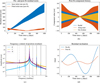 |
Fig. 6 Residuals of a 1000-day estimation of initial state. A coupled model was used for observations and an uncoupled model for estimation. Panel a: differences between the coupled and uncoupled trajectories when the same initial state is used and when the best-fit estimated initial state is used for the uncoupled model. Panel b: time history of the RSW components of residuals. Panel c: frequency content of residual components. Vertical lines indicate (integer multiples/divisors of) the mean motion (solid) and the three normal modes: longitudinal (dotted), latitudinal (dashed), and wobble (dash-dot-dot). Panel d: differences in inclination between observed and estimated trajectories. |
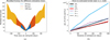 |
Fig. 7 Comparison of the results of estimations of different lengths. All of them only estimate the initial state. All of them have the same true initial state, with |ro| = 9484 km and |υo| = 2113 m/s. Panel a: residual histories for estimations of different lengths. Panel b: change in estimated initial state for estimations of different lengths (in days). |
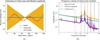 |
Fig. 8 Results in terms of residuals for an estimation of initial state and once-per-orbit libration amplitude and an estimation of initial state and gravity coefficients. The observations are generated with a coupled model and estimation is performed with an uncoupled model. Panel a: component-wise post-fit residual history of an estimation of initial state and libration amplitude. Panel b: frequency content of the S components of residuals for all three different estimations: initial state, initial state and libration amplitude, initial state and gravity coefficients. Vertical lines indicate (integer multiples/divisors of) the mean motion (solid) and the three normal modes: longitudinal (dotted), latitudinal (dashed) and wobble (dash-dot-dot). |
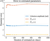 |
Fig. 9 Errors in estimated parameters for estimations performed with arcs of different lengths. Observations are generated with a coupled model and estimation is performed with an uncoupled model. Libration amplitude errors given in terms of the physical libration amplitude 𝓐 (see Sect. 2.2). |
5 Discussion
This section puts the results from this paper in the context of current and future missions and data. It assesses the impact of these results on currently available and future information on Phobos’s interior.
5.1 Libration mismodeling
The currently most robust procedure for determining the libration of Phobos, with a single once-per-orbit longitudinal libration amplitude as a free parameter in the fitting of a control point network (Burmeister et al. 2018), requires a rotational model with free parameters to fit. In our analysis, we used an uncoupled model with a single free parameter for the once-per-orbit longitudinal libration, which we show (Sect. 4.1) to most notably neglect latitudinal librations and mis-represent longitudinal librations, as a consequence both of omitting higher-order longitudinal librations, and the artificial librations induced as numerical artifacts from the use of Eq. (15b). The strongest latitudinal libration – i.e., Mars’ Phobos-fixed latitude – has an amplitude of 8.5 × 10⁻³ degrees at 27.14 rad/day (see Table 1). The uncoupled model we consider in our analysis can introduce displacements in surface points of up to 2 m. These errors, arising from a dynamical rotational model, are just below observational quality indicated by e.g., the resolution of 2.6 m/pixel of the Super Resolution Camera of Mars Express (MEX) (Oberst et al. 2014). These librations are therefore not critical in the process of currently available data, also considering the fact that the uncertainty of the once-per-orbit libration from current data is about 4 times higher (0.03 degrees) than the signature of latitudinal librations.
On the other hand, MMX will carry TENGOO, an optical camera with a 0.9 m/pixel resolution (Kameda et al. 2021). In this new scenario, latitudinal librations produced by coupled models may become significant in studies using these new images. A possible solution is to include relevant librations at the appropriate frequencies and estimate their amplitudes in the same way the once-per-orbit longitudinal libration amplitude is estimated in current bundle block adjustments. This, however, presents the complication of identifying what frequencies are relevant in the frequency spectrum – in particular for frequencies that will arise at forcings close to the normal modes. This manual and somewhat forceful introduction of frequencies into the librational spectrum of a tidally locked body such as Phobos presents several complications, thoroughly explained in Sect. 2.5.
When using the free parameters of a coupled model in the determination of a control point network (rather than one or more libration amplitudes), these issues are mitigated. Specifically, the advantage that coupled models bring in this respect lies in the fact that 7 independent scalar parameters – the independent entries in the initial rotational state vector (see Sect. 2.1) and mean moment of inertia - can represent the full libration spectrum in all three directions. This could then be used as an a priori model for a control point network. However, if one would want to use the control point network to improve the determination of the rotational dynamics, this will come at a high cost: the orbital-rotational dynamics of Phobos would need to be determined along with (or at least iteratively with) its control point network in a single inversion.
5.2 Phobos’s interior composition
Equation (24) (Dirkx et al. 2019) provides Phobos’s moments of inertia as functions of the (unnormalized) gravity coefficients C2,0 and C2,2 as well as the scaled mean moment of inertia Ĩ = I/MR2, where M and R are Phobos’s mass and reference radius. Note that Eq. (24d) relates Ĩ with the once-per-orbit longitudinal libration amplitude 𝓐. With the errors in estimated harmonic coefficients and libration amplitude from Fig. 9, the inertia moments can be mis-calculated by ~6 × 10⁻⁴ (0.4%).
 (24a)
(24a)
 (24b)
(24b)
 (24c)
(24c)
 (24d)
(24d)
Le Maistre et al. (2019) provided the values of the libration amplitude, harmonic coefficients and moments of inertia for different interior structures of Phobos – rubble pile, layered, … The moments of inertia of different structures differ by ~15%, while models are largely indistinguishable among them in terms of libration amplitude and degree 2 gravity coefficients, with the exception of the highly fractured and the disrupted-and-reaccreted bodies (both necessitating a monolithic Phobos at least at some point in time). In the light of the results of this paper, couplings will not induce a sufficient shift in estimated observables to discriminate between categories, or to draw erroneous conclusions to this respect. However, the estimation errors that may be made using an uncoupled model (using one or more libration terms) may prevent the ultimate science return of a mission from being achieved, if signatures in the data are misattributed to the incorrect parameters (Dirkx et al. 2014), as is observed in Fig. 9. The implications and nuances for future missions are discussed in Sect. 5.3.
Unlike the uncoupled models, in which one (or more) libration amplitudes are estimated, from which I and subsequently the interior structure is inferred, coupled models offer a different estimation approach. The libration amplitude itself is not directly estimated with a coupled model, but the mean moment of inertia I can be, without the intermediate determination of the libration. Similarly, the influence of the degree-two gravity field coefficients on the inertia tensor, and subsequently the body’s response to torques, is captured fully and directly by the estimation (Dirkx et al. 2019).
5.3 Future missions
Attempts at providing constraints on Phobos’s libration amplitude 𝓐 and harmonic coefficients C2,0 and C2,2 from Phobos’s orbit have been made from astrometric data (Lainey et al. 2007; Jacobson 2010; Jacobson & Lainey 2014; Lainey et al. 2021). However, as noted in their analyses, determination of one of these quantities requires fixing the other two (while determining two of them results in high correlations). As a result, ephemeris solutions are only sensitive to a linear combination of the three.
The libration amplitude has been independently determined in the creation of Phobos control point networks (Willner et al. 2014; Burmeister et al. 2018), with the latter achieving a formal uncertainty at the level of 0.03°. Radio science data from Mars Express was used by Yang et al. (2019) to estimate Phobos’s C2,0 and C2,2 concurrently, but with low statistical significance, with the analysis by Pätzold et al. (2014) stating that the signature of these parameters on the same datasets were not sufficiently strong to provide proper constraints. Geophysical knowledge of Phobos is therefore limited by the nature of available observational data, which is in turn limited by the mission profiles and instruments of spacecraft that have studied Phobos.
The determination of Phobos’s harmonic coefficients C2,0 and C2,2 will benefit greatly from tracking to a Phobos orbiter. On the one hand, the signature of these two parameters on a spacecraft orbiting Phobos is determined by the position of the spacecraft in the Phobos-fixed frame, most notably by the orbiter’s Phobos-fixed longitude λ and latitude φ (see Eq. (3)). Although these two coordinates are sensitive to Phobos’s own librations, they are dominated by the orbiter’s position in its Phobos-bound orbit. This allows us to de-correlate the estimates of libration amplitude from the estimates of harmonic coefficients. Furthermore, the two coefficients C2,0 and C2,2 have unambiguously different signals in the trajectory of a Phobos orbiter, allowing for further de-correlation of the two.
Overall, (near-)future missions (see Sect. 1), in particular those with a lander or orbiter segment, promise to change this situation. With the realization of such missions, we will have the following datasets that contain information on Phobos’s orbital and rotational dynamics:
- (i)
Camera observations of Phobos from which its orientation can be determined
- (ii)
Astrometric observations of Phobos for determination of its ephemeris
- (iii)
Radio tracking data of spacecraft near Phobos
- (iv)
Radio (or laser) tracking of a lander on Phobos.
The expected improvement in the quality and quantity of existing datasets (i)–(iii), and the addition of new datasets (iv) will allow the dynamics of Phobos, and as a result its interior to be probed to unprecedented accuracy. At present, dataset (iii) is limited to flybys, where a pseudo-orbiter would dramatically enhance the sensitivity to the gravity field (Plumaris et al. 2022). Direct-to-Earth tracking of both orbiters and landers will be sensitive to Phobos’s ephemeris, orientation and gravity field, while lander-to-orbiter tracking are (to first order) insensitive to the moon’s ephemeris. A lander can further decouple Phobos’s rotational motion in two ways, first by direct observations of Phobos’s orientation using a star-tracker, and secondly as a result of the rotation being directly visible in the tracking data, and not only due to its effect on Phobos dynamics (Le Maistre et al. 2013; Dirkx et al. 2014). The dynamics of a lander could be further constrained by measuring its relative dynamics to Martian orbiters, using methods such as same-beam Interferometry (Dehant et al. 2017) or in-beam VLBI (Fayolle et al. 2024). The best and most robust science return will be obtained from a concurrent consideration of various complementary datasets.
Specific examples of a near future Phobos mission is JAXA’s MMX (Nakamura et al. 2021; Usui et al. 2020). From this mission’s data the  and
and  gravity field coefficients could be determined to an accuracy of 0.1% (Yamamoto et al. 2024), i.e., 2.9 × 10⁻⁵ for
  and 1.6 × 10⁻⁵ for
  . At such an accuracy, our results in Fig. 9 indicate that the coupling of orbit and rotation becomes necessary to properly propagate these uncertainties (which are obtained from spacecraft tracking) into the orbital dynamics of Phobos. It has been indicated in this MMX study, and others (Yang et al. 2019, 2020), that the accurate determination of Phobos’s gravity field from spacecraft tracking data will be sensitive to errors in the ephemeris. For instance, Yamamoto et al. (2024) noted that an error of 10m in the along-track initial position of Phobos results in 2% and 5% true errors in the estimated C2,0 and C2,2 respectively, while Yang et al. (2020) reported true errors in estimated physical longitudinal libration amplitude in the order of 5 × 10⁻⁴ degrees, comparable to the true errors we find in our manuscript. Therefore, a concurrent estimation of spacecraft and moon dynamics may be necessary to fully exploit the datasets (Fayolle et al. 2022, 2023). Our results indicate that it may be necessary to consider the coupled orbital-rotational dynamics in such an approach or, at the very least, consider a more complex rotational model than a kinematic one with only a single degree of freedom.
The analyses of more speculative mission concepts involving direct-to-Earth tracking of landers by Le Maistre et al. (2013); Dirkx et al. (2014) yielded post-mission uncertainties of down to 10−5 degrees for the once-per-orbit libration. This is well below the true errors in estimation of libration amplitude reported in the present paper (see Sect. 4.2.2 and Fig. 9) originating from rotation mismodeling in the uncoupled approach. This indicates that couplings will necessarily have to be considered in the inversion of data coming from such missions. On the other hand, we show that couplings produce a drift in the along-track direction (see Sect. 4.1 and Fig. 4b), which accumulate to several meters over ~50 weeks. The effect of a meter level bias in Phobos’s ephemeris on the product of inverting Doppler data from a Phobos lander was investigated by Le Maistre et al. (2013), who found true errors in estimated libration amplitude in the order of 10−2−10−1 degrees, well above all expected formal errors. This clearly shows the relevance of using a coupled model when analyzing lander tracking data.
In their study, Dirkx et al. (2014) used a refined model of Phobos’s rotation in combination with an uncoupled translational model, featuring a total of 15 different longitudinal librations at the frequencies obtained by Rambaux et al. (2012), as well as 9 librations of Phobos’s right ascension and declination angles (in reality, the cm-level data they simulated would require significantly more terms to fully capture all effects, further exacerbating the issues that would occur in an actual mission). They estimated all amplitudes of the sine and cosine term of each libration, which amounted to a total of 66 estimated parameters to determine the orientation of Phobos. They reported extremely high correlations among them, about which they noted that it is a consequence of over-parameterizing the attitude of Phobos, which in principle would require only seven additional parameters compared to the translational dynamics: the initial orientation (three independent quantities), the initial angular velocity vector (with three entries), and the mean moment of inertia. By modeling the rotation dynamically, the rotational state is fully determined by the initial state and a differential equation of the form of Eq. (18b). The initial state has only six free parameters: three quantities specifying the orientation, three specifying the angular rates. Modeling the response to forcing torques then only requires the addition of a single parameter (compared to the translational dynamics), namely the mean moment of inertia.
The methodology of fitting the coupled orbital-rotational dynamics has been applied in the processing of Lunar Laser Ranging (LLR) data (e.g., Folkner et al. 2014), with the methodology described in detail by Mazarico et al. (2017) and Dirkx et al. (2019). The procedure was applied by Yang et al. (2024), specifically in fitting the coupled orbital-rotational dynamics to existing models of Phobos dynamics. They used the ephemeris of Lainey et al. (2021) as reference ephemeris (observations) to fit different coupled dynamical models with ever increasing complexity, such as Phobos’s deformability and higher-degree gravity coefficients, which are not included in their reference ephemeris. However, the residuals they obtained (position difference of close to 1 km over a period of 10 years, primarily consisting of short-period effects) after fitting their dynamical models to the spice kernels are far higher than those we obtain here. Unlike the results of Yang et al. (2024), the magnitude and behavior of our residuals are in line with theoretical expectations of the effect of higher-order rotation effects that are not captured by our uncoupled model. It is likely that their much higher residuals are a result of mismatches in the details of the dynamical models used in the generation of the underlying ephemeris model, and their fitting model. In doing so, the effect of translational-rotational couplings on their own is obscured by these dynamical mismatches, making it very hard to isolate the effect of couplings – which our manuscript very specifically addresses. Their high residuals are a sign of the complexities entailed in ensuring model consistency at the level required for upcoming missions such as MMX.
6 Conclusions
This paper investigates how couplings between Phobos’s translational and rotational dynamics affect the propagation of its dynamics. Furthermore, we show how using a simple, single-frequency uncoupled model in data inversion could bias the estimates of geodetic parameters of interest. The solutions of propagating an initial state with coupled and uncoupled dynamics were directly compared, and the latter model was used to estimate different parameters from observations generated by the former.
In addition to providing numerical results for the differences between the two models, we also discuss their implementation in detail. Data from future missions will require the dynamical signatures of multiple libration terms to be modeled. Extending the current uncoupled method to include them is an option, but we argue for the adoption of a coupled dynamical model in Sect. 2.5. We reiterate the core of our arguments here:
The use of the instantaneous empty focus as a reference direction (see Eq. (15)) induces spurious terms into the libration, which have an amplitude that is similar to the higher-order librations (at around 0.01 degrees, Fig. 2).
Even if the short-periodic oscillations were filtered out of the libration model, the use of the empty focus as a reference direction is not a fully correct representation of the physical effect that is to be modeled, and breaks down at O(e2).
Creating a model to overcome these issues would be possible, but would be complicated by the possible need for iterations between orbital and rotational models, with the possible issue that this may lead to small errors in the estimation (or the resulting uncertainties).
The adoption of a fully time-parametrized kinematic rotation model is complicated by the need to enforce the spinorbit resonance following a change in translational state in successive steps of the estimation.
Instead of developing higher-order uncoupled models to capture additional librations and associated estimation strategies that do not suffer from the issues listed above, the use of a self-consistent coupled orbital-rotational dynamical model is preferred. It can be incorporated into an estimation using the models presented by (Mazarico et al. 2017; Dirkx et al. 2019), and has been used in the analysis of LLR data for many years (Folkner et al. 2014). Such a model would be robust for inclusion in estimations well into the future, up to and including the use of high-accuracy lander tracking data using laser or radio tracking. Below, we summarize the quantitative results on when the use of a coupled model (or, more generally, any model more accurate than a single-libration model) becomes relevant.
As expected from theoretical predictions, we found that the dominant effect of the coupled propagation of orbit and rotation is qualitatively similar to the once-per-orbit longitudinal libration when it comes to motion inside the orbital plane. Differences between the coupled and uncoupled trajectories were largest in the along track direction, with the uncoupled solution getting ahead of the coupled one as much as 40 m after nine years and four months. However, a secular component was not present in the differences in the radial and out-of-plane directions, which oscillated with a growing amplitude that reached 4 m.
The largest longitudinal and latitudinal librations that the simplified, single-frequency uncoupled model does not account for stand at amplitudes of 3.6 × 10⁻³ and 8.5 × 10⁻³ degrees, respectively – displacements at Phobos’s surface of 0.8 and 1.9 meters, respectively. While the additional longitudinal librations cause a drift in along-track position, latitudinal librations couple with Phobos’s orbit to produce an ever-growing oscillation of Phobos’s inclination with a period of about two years, which in turn induces long-term librations that are not accounted for by a single-frequency uncoupled model as typically used in orbital studies of Phobos. Finally, as illustrated in Fig. 2, extra libration signals at multiples of the orbital frequency are artificially introduced by the classical uncoupled implementation (Eq. (15)). These additional signatures are automatically absent from a fully consistent translational-rotational solution, which highlights yet another advantage of a coupled propagation.
The largest post-fit residuals were seen to occur mostly in the out-of-plane direction, in which the once-per-orbit longitudinal libration and Phobos’s zonal and sectorial gravity coefficients of degree 2 have little to no effect, and cannot absorb the mismodeling of the rotation. They showed the largest values at 45 cm at the two ends of the 1000-day arc. Along-track residuals showed a long-periodic oscillation that could potentially outgrow the out-of-plane components for longer estimations. Further study is required in this direction.
Finally, mismodeling of the moon’s rotation in the estimation (which originates from neglected libration components, and/or translational-rotational couplings) makes the estimated parameters deviate from their true values. These true errors should ideally stay below formal errors. True errors in the amplitude of the once-per-orbit physical longitudinal libration 𝓐 and Phobos’s normalized coefficients  and
and  were found to be of about 1.58 × 10⁻³ degrees, 6.6 × 10⁻⁵ and 1.1 × 10⁻⁵ respectively after 1000 days. All these true errors are well within the error bars of current inversion products, but are one to three orders of magnitude above the expected formal errors computed by Dirkx et al. (2014) for a lander ranging concept. This type of observation represents the limiting factor in a likely Phobos-bound mission that provides lander and orbiter range measurements. These data will be most fruitfully processed together as a single observation set. Thus, a proper inversion of these data will not be possible with the use of the same uncoupled models that have been customary until now. For this, a more refined rotational model is necessary. As we argue above, a coupled translational-rotational model is best suited for such high-fidelity applications, as it provides a more robust determination of the coupled dynamics while ensuring that all physical effects are correctly captured in the quantification of the post-fit uncertainties of the interior properties.
Acknowledgements
We thank two anonymous reviewers for their detailed comments on our manuscript, which greatly improved our discussion and argumentation. Part of the work performed after the defense of the MSc thesis that resulted in this paper was performed under the GRACEFUL Synergy Grant (agreement No. 855677), funded by the ERC’s Horizon 2020 research and innovation program.
Appendix A Complete simulation definition
Here, we summarize the specific models we have used in our equations of motion.
In the evaluation of all the terms in the equations of motion, the positions of all bodies is required, as well as their gravitational parameters and, in some cases, their harmonic coefficients as well. The rest of this section will specify the sources of all this data used in this work.
A.1 Mars
Gravity field: MRO120D developed by Konopliv et al. (2016). Mars’ reference radius (R in Eq. (3b)) is 3396.0km and the Martian gravitational parameter is µM = 42828.3750104 km3/s2. All sine and cosine coefficients up to degree and order 12 have been included.
Rotation model: The rotation model developed by Konopliv et al. (2016), used also by Lainey et al. (2021).
A.2 Phobos
Gravity field: Quadrupole gravity field, using only
 and
and  , taken from the homogeneous model of Phobos by Le Maistre et al. (2019). The reference radius is 14km and the mass is 1.06 × 10¹⁶kg. A value of G = 6.67259 × 10⁻¹¹ was used, resulting in µP = 707294.54m3/s2.
Rotation model: See Sect. 2.4.
Inertia tensor: Computed with the gravity coefficients as per Eq. (A.1) (Le Maistre et al. 2019), where Ĩ is the mean moment of inertia. These moments are normalized with MR2. In this work, the value of Ĩ was selected to be consistent with the homogeneous model of Phobos. The full tensor for a gravity field containing all coefficients up to degree and order 2 is provided in Eq. (23) by Le Maistre et al. (2019), from which a normalized mean moment of inertia of Ĩ = 0.2645233 can be inferred.
 (A.1)
(A.1)
A.3 Third bodies
Sun, Jupiter and Earth: The masses of these bodies are taken from the INPOP19a (Fienga et al. 2019) ephemerides product. Their locations are computed with a combination of the NOE-4-2020 ephemerides (Lainey et al. 2021) within the Martian system.
Deimos: The mass and position of Deimos are computed with the NOE-4-2020 ephemerides (Lainey et al. 2021).
A.4 Numerical integration
All these equations and terms have been numerically propagated using Tudat (TU Delft Astrodynamics Toolbox), which offers a wide range of possible integrators, propagators and environments, and has been used for a range of analyses related to the dynamics of natural satellites, and their estimation (Dirkx et al. 2014, 2016; Plumaris et al. 2022; Fayolle et al. 2022, 2023, 2024). In this work, all simulations have been performed using the Cowell propagator formulated in Eq. (9) in combination with an RKF8(10) integrator working in a fixed-step regime of 5 minutes. For reproducibility purposes, Eq. (A.2) provides the translational and rotational initial states returned by the damping algorithm discussed in Sect. 2.3 and described in B. The translational state has been used for both the coupled and uncoupled models in propagation. We (arbitrarily) set our initial time to the epoch J2000.
![Mathematical equation: ${x_{t,o}} = \left[ {\matrix{ { - 1991723.0176246795} \hfill \cr { - 8742964.680527888} \hfill \cr { - 3180540.016758049} \hfill \cr {1843.0987517454296} \hfill \cr { - 43.60246872601227} \hfill \cr { - 1018.5417927808861} \hfill \cr } } \right]$](/articles/aa/full_html/2025/08/aa50579-24/aa50579-24-eq66.png) (A.2a)
(A.2a)
![Mathematical equation: ${x_{r,o}} = \left[ {\matrix{ {0.7117384685576372} \cr {0.3074341368827725} \cr {0.0347308749007907} \cr {0.6306396516101695} \cr {6.2438591968356885 \times {{10}^{ - 9}}} \cr { - 1.3079675754811962 \times {{10}^{ - 7}}} \cr {2.323693355272973 \times {{10}^{ - 4}}} \cr } } \right]$](/articles/aa/full_html/2025/08/aa50579-24/aa50579-24-eq67.png) (A.2b)
(A.2b)
Appendix B Damping algorithm
The damping algorithm used in this work is that used by Rambaux et al. (2012). This algorithm is heavily particularized for obtaining an initial state of bodies that are locked in spin-orbit resonance and present a constant (averaged) rotation around their z axis. Such a constant rotation rate will follow the evolution of their orbital mean motion, and will be denoted here as ωo. The algorithm is designed to damp the normal modes around all axes, while preserving this constant rotation.
For this, a virtual torque is added to the dynamics of the moon, which is known to oppose its rotation. This virtual torque Γd is computed as in Eq. (B.1).
 (B.1)
(B.1)
In this equation, τd is a given dissipation time that is provided by the user, I is the body’s inertia tensor (in body axes), ω = [ωx, ωy, ωz] is the rotational velocity of the moon (expressed in body axes) and ωo = [0, 0, ωo] is the constant angular velocity of a moon in pure synchronous rotation.
In order to obtain the damped dynamics of the moon, the algorithm propagates the dynamics with the torque forward in time for a time of 10τd. The final state is used to start a propagation backward in time and without the virtual torque. The result of this forward-backward propagation is a damped initial state at t = 0 that, if propagated forward in time without the virtual torque, the dynamics will not contain the normal modes.
Or at least, not in such a strong way as before the two propagations. The damping provided by the virtual torque is not perfect, so the process is repeated several times with ever-increasing dissipation times. Each iteration, the damped initial state from the previous iteration is used to propagate the dynamics forward with the damping torque. This way, the initial state is damped even further in each iteration.
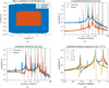 |
Fig. B.1 Damping algorithm explained in figures. Vertical lines indicate (integer multiples/divisors of) the mean motion (solid) and all three normal modes: longitudinal (dotted), latitudinal (dashed) and wobble (dash-dot-dot). Panel a: Comparison between damped and undamped tidal librations. Panel b: Frequency content of Phobos-fixed longitude of Mars for both the damped and undamped dynamics. Panel c: Frequency content of Phobos-fixed latitude of Mars for both the damped and undamped dynamics. Panel d: Damping process of the latitudinal librations close to the latitudinal normal mode. |
The process and result of this damping algorithm is portrayed in Fig. B.1. In this work, an initial value of τd = 4h has been used, and each iteration of the damping algorithm doubles this damping time, up to a final damping time of τd = 8192h. Note that a value of τd = ∞ means there is no damping at all. In Fig. B.1a, the Phobos-fixed angular coordinates of Mars – i.e., the moon-to-planet line – are plotted in a longitude-latitude map, where the (0,0) coordinate is identified with the Phobos’s long axis. Here the overall effect of the full damping algorithm is very well represented. Pre-algorithm dynamics feature Phobos’s x-axis deviating from the moon-to-planet line about 4.5° in longitude and almost 0.04° in latitude, product of a mixture of normal modes together with resonant forcings. The damping algorithm removes all oscillations occurring at the frequencies of the normal modes while leaving all librations due to forcings behind, as well as the once-per-orbit longitudinal libration.
The difference in the frequency spectra of the damped and undamped librational motions of Phobos are presented in Fig. B.1b and Fig. B.1c respectively. Recall that the virtual torque (Eq. (B.1)) is designed to oppose all rotational motion except the constant, uniform rotation at the orbital frequency. The motion after backward propagation (without damping torque) reintroduces all forced librations, as they are excited by the naturally occurring torques. Since the free librations are largely damped in the forward propagation (just like the forced ones), and no mechanism to re-excite them is included in the backward propagation, their amplitudes are substantially diminished. Repetition of this forward-backward propagation will thus damp free librations over increasingly long timescales, while maintaining the forced librations.
Note, however, that each of these iterations involves the re-propagation of the full translational-rotational dynamics with an initial state adjusted to reduce the amplitude of the free modes. A reduction in free libration amplitude at the initial condition will impact the full translational-rotational state, and consequently the orbital and rotational forcing, leading to a change in the full resulting coupled state history. Therefore, the damping algorithm does not influence only the terms at the free libration frequencies, but the entire libration spectrum. For the case of Phobos, this is particularly important because normal modes are very close to these frequencies, leading to strong coupling between free and forced rotational motion. This is clearly observed in Fig. B.1b, where it can be seen that the once-per-orbit forced libration is significantly different in the undamped case. Crucially, this forced libration amplitude differs significantly from the theoretically predicted value, while the amplitude in the damped case matches expectations very closely (see Sect. 4.1.2). This shows that the damping algorithm is crucial to make the full librati onal spectrum (not just the amplitudes at the free modes) representative of the real situation.
For illustration, the progressive damping of one of the latitudinal librations can be seen in Fig. B.1d. A first, undamped simulation (τ = ∞) contains both free and forced librations around the frequency of the latitudinal normal mode. Subsequent iterations of the damping algorithm described here reduce the amplitude of most of these peaks to ~ 0.1 mdeg – what we have considered floor noise level in our coupled model. These librations that disappear over the course of the damping algorithm are therefore interpreted as free librations, while the peak that retains its full amplitude over the whole damping process is interpreted as a forced libration. As a matter of fact, this is the forced libration occurring at ~ 27.15 rad/day that is reported in Table 1 and attributed to the twice-synodic frequency between Phobos’s orbit and the Martian rotation (see Sect. 4.1.2).
References
- Archinal, B. A., Acton, C. H., A’Hearn, M. F., et al. 2018, Celest. Mech. Dyn. Astron., 130, 22 [Google Scholar]
- Bagheri, A., Khan, A., Efroimsky, M., Kruglyakov, M., & Giardini, D. 2021, Nat. Astron., 5, 539 [NASA ADS] [CrossRef] [Google Scholar]
- Baland, R.-M., Yseboodt, M., & Van Hoolst, T. 2012, Icarus, 220, 435 [NASA ADS] [CrossRef] [Google Scholar]
- Borderies, N. 1977, Celest. Mech., 18, 295 [Google Scholar]
- Borderies, N., & Yoder, C. 1990, A&A, 233, 235 [NASA ADS] [Google Scholar]
- Burmeister, S., Willner, K., Schmidt, V., & Oberst, J. 2018, J. Geodesy, 92, 963 [Google Scholar]
- Chapront, J., Chapront-Touzé, M., & Francou, G. 1999a, Celest. Mech. Dyn. Astron., 73, 317 [Google Scholar]
- Chapront, J., Chapront-Touzé, M., & Francou, G. 1999b, A&A, 343, 624 [NASA ADS] [Google Scholar]
- Chapront-Touze, M. 1990, AAP, 235, 447 [Google Scholar]
- Chen, H., Rambaux, N., Lainey, V., & Hestroffer, D. 2022, Rem. Sens., 14, 1619 [Google Scholar]
- Dehant, V., Park, R., Dirkx, D., et al. 2017, Space Sci. Rev., 212, 1433 [NASA ADS] [CrossRef] [Google Scholar]
- Dirkx, D., Vermeersen, L., Noomen, R., & Visser, P. 2014, Planet. Space Sci., 99, 84 [Google Scholar]
- Dirkx, D., Lainey, V., Gurvits, L., & Visser, P. 2016, Planet. Space Sci., 134, 82 [Google Scholar]
- Dirkx, D., Mooij, E., & Root, B. 2019, Astrophys. Space Sci., 364, 37 [Google Scholar]
- Dirkx, D., Fayolle, M., Garrett, G., et al. 2022, EPSC2022, 16 [Google Scholar]
- Duxbury, T. C., & Callahan, J. D. 1981, AJ, 86, 1722 [Google Scholar]
- Fayolle, S. 2025, PhD thesis, Delft University of Technology [Google Scholar]
- Fayolle, M., Dirkx, D., Lainey, V., Gurvits, L., & Visser, P. 2022, Planet. Space Sci., 219, 105531 [CrossRef] [Google Scholar]
- Fayolle, M., Magnanini, A., Lainey, V., et al. 2023, A&A, 677, A42 [NASA ADS] [CrossRef] [EDP Sciences] [Google Scholar]
- Fayolle, M. S., Dirkx, D., Cimo, G., et al. 2024, Icarus, 416, 116101 [Google Scholar]
- Feagin, T. 2012, Neural Parallel Sci. Computat., 20, 437 [Google Scholar]
- Fienga, A., Avdellidou, C., & Hanuš, J. 2019, MNRAS, 492, 589 [Google Scholar]
- Folkner, W. M., Williams, J. G., Boggs, D. H., Park, R. S., & Kuchynka, P. 2014, Interplanetary Network Progress Report, 42-196, 1 [Google Scholar]
- Fukushima, T. 2012, AJ, 135, 2298 [Google Scholar]
- Goli, M., Le Maistre, S., & Yseboodt, M. 2024, Planet. Space Sci., 251, 105958 [Google Scholar]
- Guo, X., Yan, J., Yang, X., et al. 2023, MNRAS, 520, 925 [Google Scholar]
- Hall, A. 1878, MNRAS, 38, 205 [Google Scholar]
- Jacobson, R. A. 2010, AJ, 139, 668 [Google Scholar]
- Jacobson, R., & Lainey, V. 2014, Planet. Space Sci., 102, 35 [CrossRef] [Google Scholar]
- Jacobson, R., Konopliv, A., Park, R., & Folkner, W. 2018, Planet. Space Sci., 152, 107 [Google Scholar]
- Kameda, S., Ozaki, M., Enya, K., et al. 2021, Earth Planets Space, 73, 218 [Google Scholar]
- Keeler, J. E. 1888, AJ, 8, 73 [Google Scholar]
- Konopliv, A. S., Park, R. S., & Folkner, W. M. 2016, Icarus, 274, 253 [Google Scholar]
- Lainey, V., Duriez, L., & Vienne, A. 2004, A&A, 420, 1171 [NASA ADS] [CrossRef] [EDP Sciences] [Google Scholar]
- Lainey, V., Dehant, V., & Pätzold, M. 2007, A&A, 465, 1075 [NASA ADS] [CrossRef] [EDP Sciences] [Google Scholar]
- Lainey, V., Noyelles, B., Cooper, N., et al. 2019, Icarus, 326, 48 [Google Scholar]
- Lainey, V., Pasewaldt, A., Robert, V., et al. 2021, A&A, 650, A64 [NASA ADS] [CrossRef] [EDP Sciences] [Google Scholar]
- Le Maistre, S., Rosenblatt, P., Rambaux, N., et al. 2013, Planet. Space Sci., 85, 106 [NASA ADS] [CrossRef] [Google Scholar]
- Le Maistre, S., Rivoldini, A., & Rosenblatt, P. 2019, Icarus, 321, 272 [NASA ADS] [CrossRef] [Google Scholar]
- Le Maistre, S., Rivoldini, A., Caldiero, A., et al. 2023, Nature, 619, 733 [Google Scholar]
- Marov, M., Avduevsky, V., Akim, E., et al. 2004, Adv. Space Res., 33, 2276 [NASA ADS] [CrossRef] [Google Scholar]
- Marth, A. 1879, Astron. Nachr., 95, 369 [Google Scholar]
- Mazarico, E., Rowlands, D. D., Sabaka, T. J., et al. 2017, J. Geodesy, 91, 1141 [Google Scholar]
- Miranda, C., Patel, M., Berberan-Santos, M. N., et al. 2023, Front. Astron. Space Sci., 10 [Google Scholar]
- Murray, C. D., & Dermott, S. F. 1999, Solar System Dynamics (Cambridge university press) [Google Scholar]
- Nakamura, T., Ikeda, H., Kouyama, T., et al. 2021, Earth Planets Space, 73, 227 [NASA ADS] [CrossRef] [Google Scholar]
- Newall, H. F. 1895, MNRAS, 55, 348 [Google Scholar]
- Newhall, X., Standish, E. M., & Williams, J. G. 1983, A&A, 125, 150 [Google Scholar]
- Oberst, J., Lainey, V., Poncin-Lafitte, C. L., et al. 2012, Exp. Astron., 34, 243 [Google Scholar]
- Oberst, J., Zubarev, A., Nadezhdina, I., Shishkina, L., & Rambaux, N. 2014, Planet. Space Sci., 102, 45 [NASA ADS] [CrossRef] [Google Scholar]
- Pätzold, M., Andert, T., Jacobson, R., Rosenblatt, P., & Dehant, V. 2014, Planet. Space Sci., 102, 86 [Google Scholar]
- Petit, G., Luzum, B., et al. 2010, https://www.iers.org/IERS/EN/ Publications/TechnicalNotes/tn36.html [Google Scholar]
- Pickering, E. C., Searle, A., & Upton, W. 1879, Ann. Harvard Coll. Observ., 11, 311 [Google Scholar]
- Plumaris, M., Dirkx, D., Siemes, C., & Carraz, O. 2022, Rem. Sens., 14, 3030 [Google Scholar]
- Rambaux, N., & Williams, J. 2011, Celest. Mech. Dyn. Astron., 109, 85 [NASA ADS] [CrossRef] [Google Scholar]
- Rambaux, N., Castillo-Rogez, J. C., Williams, J. G., & Özgür Karatekin. 2010, Geophys. Res. Lett., 37, 4202 [NASA ADS] [CrossRef] [Google Scholar]
- Rambaux, N., Van Hoolst, T., & Karatekin, O. 2011, A&A, 527, A118 [NASA ADS] [CrossRef] [EDP Sciences] [Google Scholar]
- Rambaux, N., Castillo-Rogez, J. C., Le Maistre, S., & Rosenblatt, P. 2012, A&A, 548, A14 [NASA ADS] [CrossRef] [EDP Sciences] [Google Scholar]
- Rosenblatt, P., Charnoz, S., Dunseath, K. M., et al. 2016, Nat. Geosci., 9, 581 [NASA ADS] [CrossRef] [Google Scholar]
- Smith, B. A. 1970, Science, 168, 828 [Google Scholar]
- Stark, A., Willner, K., Burmeister, S., & Oberst, J. 2017, in European Planetary Science Congress 2017, 11, EPSC2017-868-1 [Google Scholar]
- Usui, T., Bajo, K.-i., Fujiya, W., et al. 2020, Space Sci. Rev., 216, 49 [Google Scholar]
- Veverka, J. 1978, Vistas Astron., 22, 163 [Google Scholar]
- Willner, K., Oberst, J., Hussmann, H., et al. 2010, Earth Planet. Sci. Lett., 294, 541 [Google Scholar]
- Willner, K., Shi, X., & Oberst, J. 2014, Planet. Space Sci., 102, 51 [Google Scholar]
- Woolard, E. W. 1944, AJ, 51, 33 [Google Scholar]
- Yamamoto, K., Matsumoto, K., Ikeda, H., et al. 2024, Earth, Planets and Space, 76, 1 [Google Scholar]
- Yang, X., Yan, J. G., Andert, T., et al. 2019, MNRAS, 490, 2007 [NASA ADS] [CrossRef] [Google Scholar]
- Yang, Y., Yan, J., Guo, X., He, Q., & Barriot, J.-P. 2020, A&A, 636, A27 [NASA ADS] [CrossRef] [EDP Sciences] [Google Scholar]
- Yang, Y., Yan, J., Jian, N., et al. 2024, A&A, 685, A13 [NASA ADS] [CrossRef] [EDP Sciences] [Google Scholar]
- Zhong, Z., Wen, Q., Yan, J., & Pang, L. 2023, Rem. Sens., 15, 3162 [Google Scholar]
The sign convention we use for Eq. (11) is the same as that of Lainey et al. (2019, 2021). Other analyses, such as that by Jacobson (2010), choose a different positive direction for one or more of the angles.
Note that Rambaux et al. (2012) used a different angle decomposition and reference frame than we do here.
All Tables
Main peaks of the tidal longitudinal libration as computed by the uncoupled model.
All Figures
|
Fig. 1 Librational geometry, where θ and M are the true and mean anomalies of Phobos in its orbit, ψ is the tidal libration angle, γ is the physical libration angle, and F′ represents the empty focus of the ellipse. The angle between the moon-to-empty-focus and the apse lines is equal to M up to O(e2) (Murray & Dermott 1999). The eccentricity of this figure has been greatly exaggerated for visualization purposes. |
| In the text | |
|
Fig. 2 Frequency content of the tidal longitudinal libration of an uncoupled translational state in which a fully locked configuration of Phobos has been assumed, together with a once-per-orbit longitudinal libration. |
| In the text | |
|
Fig. 3 Schematic of the work done in this paper. |
| In the text | |
|
Fig. 4 Propagation results. The differences in position is studied in different ways: norm (panel a), components (panel b), frequency content (panel c) and Keplerian elements (panel d). Vertical lines in the bottom left picture represent (multiples of) the mean motion (n) and latitudinal normal mode (ωlat). Here, the coupled states have been subtracted from the uncoupled ones. Panel a: norm of position difference between the states propagated by the uncoupled model and those propagated by the coupled model. Panel b: time evolution of the RSW components of the position differences between the coupled and uncoupled trajectories. Panel c: frequency content of the RSW components of the position differences between the coupled and uncoupled trajectories. Panel d: differences in inclination between the coupled and uncoupled trajectories. |
| In the text | |
|
Fig. 5 Comparison of the position differences between the coupled and uncoupled trajectories (blue) and the position differences between the classical uncoupled model (i.e., with once-per-orbit libration) and fully locked (i.e., no libration) trajectories (orange). Only the final ten orbits of the nine years and four months have been plotted. Note the different units. Panel a: in-plane projection of position differences. Panel b: out-oſ-plane projection of position differences. |
| In the text | |
|
Fig. 6 Residuals of a 1000-day estimation of initial state. A coupled model was used for observations and an uncoupled model for estimation. Panel a: differences between the coupled and uncoupled trajectories when the same initial state is used and when the best-fit estimated initial state is used for the uncoupled model. Panel b: time history of the RSW components of residuals. Panel c: frequency content of residual components. Vertical lines indicate (integer multiples/divisors of) the mean motion (solid) and the three normal modes: longitudinal (dotted), latitudinal (dashed), and wobble (dash-dot-dot). Panel d: differences in inclination between observed and estimated trajectories. |
| In the text | |
|
Fig. 7 Comparison of the results of estimations of different lengths. All of them only estimate the initial state. All of them have the same true initial state, with |ro| = 9484 km and |υo| = 2113 m/s. Panel a: residual histories for estimations of different lengths. Panel b: change in estimated initial state for estimations of different lengths (in days). |
| In the text | |
|
Fig. 8 Results in terms of residuals for an estimation of initial state and once-per-orbit libration amplitude and an estimation of initial state and gravity coefficients. The observations are generated with a coupled model and estimation is performed with an uncoupled model. Panel a: component-wise post-fit residual history of an estimation of initial state and libration amplitude. Panel b: frequency content of the S components of residuals for all three different estimations: initial state, initial state and libration amplitude, initial state and gravity coefficients. Vertical lines indicate (integer multiples/divisors of) the mean motion (solid) and the three normal modes: longitudinal (dotted), latitudinal (dashed) and wobble (dash-dot-dot). |
| In the text | |
|
Fig. 9 Errors in estimated parameters for estimations performed with arcs of different lengths. Observations are generated with a coupled model and estimation is performed with an uncoupled model. Libration amplitude errors given in terms of the physical libration amplitude 𝓐 (see Sect. 2.2). |
| In the text | |
|
Fig. B.1 Damping algorithm explained in figures. Vertical lines indicate (integer multiples/divisors of) the mean motion (solid) and all three normal modes: longitudinal (dotted), latitudinal (dashed) and wobble (dash-dot-dot). Panel a: Comparison between damped and undamped tidal librations. Panel b: Frequency content of Phobos-fixed longitude of Mars for both the damped and undamped dynamics. Panel c: Frequency content of Phobos-fixed latitude of Mars for both the damped and undamped dynamics. Panel d: Damping process of the latitudinal librations close to the latitudinal normal mode. |
| In the text | |
Current usage metrics show cumulative count of Article Views (full-text article views including HTML views, PDF and ePub downloads, according to the available data) and Abstracts Views on Vision4Press platform.
Data correspond to usage on the plateform after 2015. The current usage metrics is available 48-96 hours after online publication and is updated daily on week days.
Initial download of the metrics may take a while.