| Issue |
A&A
Volume 700, August 2025
|
|
|---|---|---|
| Article Number | A86 | |
| Number of page(s) | 11 | |
| Section | Planets, planetary systems, and small bodies | |
| DOI | https://doi.org/10.1051/0004-6361/202451466 | |
| Published online | 06 August 2025 | |
Reanalysis of the Huygens GCMS dataset
II. Trace species in Titan's lower atmosphere
1
LATMOS-IPSL, CNRS, Sorbonne université, UVSQ Université Paris-Saclay,
France
2
LESIA, Observatoire de Paris, Université PSL, Sorbonne Université, Université Paris Cité, CNRS,
Meudon,
France
3
Department of Earth and Planetary Sciences, Johns Hopkins University,
Baltimore,
MD,
USA
4
Groupe de Spectroscopie Moléculaire et Atmosphérique (GSMA), Université de Reims Champagne-Ardenne,
Reims,
France
★ Corresponding author.
Received:
11
July
2024
Accepted:
28
March
2025
Abstract
The Huygens probe landed on Titan in January 2005, following the arrival of the Cassini-Huygens mission in the Kronian system. The Gas Chromatograph Mass Spectrometer instrument (GCMS) aboard the Huygens probe performed measurements in the lower stratosphere (from an altitude of 150 km) and in the troposphere to constrain the composition of Titan’s atmosphere. Earlier works on this dataset focused mainly on the major constituents of Titan atmosphere and on noble gases and were not able to quantify the trace gas composition in the atmosphere because of limitations in their mass spectrometry (MS) analysis techniques. In this paper, the GCMS dataset was analyzed with a MS deconvolution code that uses a Monte Carlo approach to quantify these trace gases. The mole fractions of four trace species retrieved from the GCMS data are significantly higher than the ones retrieved by the inversion of data returned by the Cassini-Composite InfraRed Spectrometer (CIRS) and the mixing ratio predicted for these volatiles by the Titan Planetary Climate model. As such, our results do not match with anything that we know of Titan’s lower atmosphere, which very likely points toward the fact that the GCMS instrument did not in fact measure atmospheric trace gases only. We investigated several hypotheses that could explain this discrepancy. In our opinion, the most likely one is that the trace gases measured by GCMS correspond to an outgassing from Titan atmospheric aerosols that could have been trapped inside the instrument. However, mole fractions of trace species retrieved from GCMS Leak 3 measurements matched with CIRS retrieved values and modeled data, and these are the only atmospheric trace gas measurements from Huygens GCMS. This dataset can be used further to identify other minor species present in this atmospheric region.
Key words: planets and satellites: atmospheres
© The Authors 2025
 Open Access article, published by EDP Sciences, under the terms of the Creative Commons Attribution License (https://creativecommons.org/licenses/by/4.0), which permits unrestricted use, distribution, and reproduction in any medium, provided the original work is properly cited.
This article is published in open access under the Subscribe to Open model. This email address is being protected from spambots. You need JavaScript enabled to view it. to support open access publication.
1 Introduction
Titan, the largest moon of Saturn, is the only moon in the Solar System to have a thick atmosphere (e.g., Hörst 2017; Hunten 1978; Nixon 2024). It is mainly composed of molecular nitrogen (N2) and methane (CH4). These two gases are photolyzed and ionized at very high altitudes primarily by solar photons and associated photoelectrons (e.g., Galand et al. 2006; Robertson et al. 2009). The reactions eventually result in the production of a variety of compounds, mostly hydrocarbons and nitriles, through a complex atmospheric chemistry.
For example, methane photo dissociation leads to the formation of ethane, which undergoes further chemistry to form acetylene and ethylene. These two species can then further react to form larger molecules. Similarly, dinitrogen gets photolyzed, enabling nitrogenous chemistry whereby one of the first steps is the formation of hydrogen cyanide followed by other nitrogenbearing species, especially nitriles (e.g., Vuitton et al. 2019). The dissociation of methane results in its net loss in the upper atmosphere, since most of the hydrogen escapes from the atmosphere. This implies a relatively short lifetime for methane in Titan’s atmosphere, making its existence above the percent level a mystery to this day (Lunine & Atreya 2008). Hydrocarbons and nitriles formed at high altitudes can then recombine to form larger molecules, which themselves can recombine to form larger molecules and so on, until reaching the formation of solid aerosol particles several hundreds to thousands of daltons (Da) in size, such as the ones detected by the CAPS instrument (Coates et al. 2007; Waite Jr et al. 2007) in the ionosphere. While the exact formation pathways of the aerosols are not fully constrained yet, polyaromatic hydrocarbons (PAH) and nitrogen-bearing PAH (PANH) likely play a role in the formation of the macromolecular polymer that will result in the aerosols. Aerosols formed at high altitudes then travel downward in the atmosphere (Lavvas et al. 2011), eventually forming a several-hundred-kilometer-thick layered structure all around Titan. While the main aerosol layer was in the high stratosphere around 500km in the early Cassini phase (Porco et al. 2005), aerosols also sediment toward the lower atmosphere and eventually reach Titan’s surface. In addition to aerosol sedimentation, the gaseous products resulting from the intense high altitude photochemistry are also vertically and horizontally transported in Titan’s atmosphere through atmospheric dynamics and were detected in the lower stratosphere with the CIRS instrument (e.g., Vinatier et al. 2015; Mathé et al. 2020). Because of the tropopause thermal inversion, the hydrocarbons and nitriles present in their gaseous form in the stratosphere are then expected to condense in the high troposphere. In contrast to the organic compounds, noble gases like argon and neon are chemically inert, expected to be well mixed, and are good proxies for studying the various dynamics taking place in Titan’s atmosphere and influencing the distribution of reactive species.
The Cassini-Huygens mission, launched in 1997, reached the Saturn system by 2004. The Huygens probe attached to the orbiter was released in December 2004, and on January 14, 2005, entered the atmosphere of Titan (Lebreton & Matson 2002; Clausen et al. 2002; Lebreton 2018). The probe had several science instruments, one of which was the Gas Chromatograph Mass Spectrometer (GCMS) (Niemann et al. 2002) that measured the atmospheric composition of different gases during the descent. This was the only mission that obtained in situ measurements of the lower atmosphere of Titan.
Data from the GCMS was used to determine the vertical profile of methane in the lower atmosphere with possible evidence of its outgassing from the surface (Niemann et al. 2005). Niemann et al. (2010) published a follow-up paper with profiles of molecular hydrogen gas and of some trace gases (C2H6, C2H2, CO2, C2N2, Ar, and Ne). The profiles of the four carbon species could not be significantly calculated before touchdown at the surface and the noble gas composition was also calculated only at specific altitudes. Hence, there is a need to constrain the atmospheric composition of trace species from this dataset to understand the characteristics of the lower atmosphere. In this paper, we analyze the vertical profiles of mole fractions of five species measured by the GCMS, using a mass spectrometry (MS) deconvolution technique (Gautier et al. 2020) that has been used to compute the methane vertical profile in Gautier et al. (2024). This is the first time that mole fractions of trace species could be computed from GCMS measurements in the entire atmospheric column.
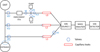 |
Fig. 1 Schematic diagram of gas flow inside the GCMS through ion source 1. The eight blue hexagons and three red cylinders are the valves and leaks, respectively, and they have been labeled similarly to the instrument diagram in Niemann et al. (2002) paper. Gas flows through L1, L2, and L3 at different times during the mission. The valves were used for specific purposes and their functions are mentioned in Niemann et al. (2002). Dotted blue circles represent the possible sources of aerosol accumulation in the GCMS (explained in Section 4.2.3) |
2 Methodology
2.1 Functioning of GCMS
The GCMS started sampling the atmosphere from an altitude of 147 km. It sampled for nearly 3.5 hours - with 2.5 hours in the atmosphere and around an hour on the surface (Niemann et al. 2010; Clausen et al. 2002; Lebreton & Matson 2002). The inlet (entrance) and the outlet (exit) were located at the bottom and top of the probe, respectively, to avoid contamination by the exhaust at the outlet. The pressure inside was kept lower than the ambient pressure to create a pressure differential, allowing gas to flow smoothly inside the instrument (Niemann et al. 2002, 2010).
There were five ion sources inside the instrument. One of them was connected to the line that directly sampled from the atmosphere, one was connected to the Aerosol Collector and Pyrolyser (ACP) instrument that was used for aerosol studies, and the rest were connected to three gas chromatographic columns for GC analysis. In our work, we are concerned with the first ion source connected directly to the inlet (see Figure 1). The atmospheric gas enters the instrument because of the pressure difference between the inlet and exit, flows through the valves and capillary leaks toward the ion source, where they were ionized by electron ionization at 70 eV. We note that 70 eV electron ionization induces the fragmentation of incoming molecules and the formation of secondary ions, called fragments. These ions and fragments were then sent to a quadrupole mass analyzer for mass filtering by varying the voltage to detect count rates for each mass-to-charge ratio (m/z) between 2 and 141 u. Ions were then sent to one of the two secondary electron multiplier (SEM) detectors for counting. The detectors then stored these count rates in a 16-bit data format and these were then transmitted back for interpretation (Niemann et al. 2010).
The data was uncompressed and processed by the original GCMS team. For ion source 1, we have data from the three leaks (L1, L2, and L3, as is shown in Figure 1) that were used at different times during the science operations. These leaks were made of a series of seven capillaries of different sizes to allow gas to flow smoothly toward the ion source (Niemann et al. 2002). Leak 1 was used during lower pressure in the atmosphere from the start of operation (at an altitude of 147 km) until about 1746 s (66 km) and leak 2 was used at higher pressure in the atmosphere from 2164 s (55 km) until the end of the mission on the surface. A part of the sampled atmosphere between 75 and 73 km (approximately 44 seconds) was sent to the enrichment cell (EC) to conduct noble gases and trace gases experiments. These gases were then sent via leak 3 for MS analysis between 66 and 55 km. The detailed execution of these scientific operations is mentioned in DESC_FM_08F.pdf, available in NASA PDS (Team HUYGENS GCMS 2006b). Background measurements were also conducted for a few seconds before the operation of each leak.
Leak 1 was simultaneously sampling from the atmosphere while the EC (connected to Leak 3) was filling up. There was a sudden increase in Leak 1 sampled count rates for all mass peaks just after the closing of the cell, and this continued until the end of the leak’s operation. This increase was attributed to the failure of a GC column at 74 km, which caused a sensitivity change in ion source 1 measurements (Niemann et al. 2010). A closer look at the data showed that the increase happened exactly after the EC closed at 73 km. Hence, it is possible that, along with the sensitivity change, the closing of the valve connected to the EC might have caused a pressure change in Leak 1, which led to increased count rates. This change was similar for all masses, and hence has not affected mole fraction computations of species considered in this work.
2.2 Data treatment
The processed GCMS data files did not contain the altitude, ambient pressure, and temperature measurements because the instrument was not programmed to measure them during the descent. These physical parameters were measured by the Huygens Atmospheric Structure Instrument (HASI) (Fulchignoni et al. 2002) on board the probe and were interpolated into the GCMS files. The measured mass spectra had to be corrected to account for several instrumental issues. The first step was to correct the piling up of ions at the detector (Niemann et al. 2010). After every detection, the detector needs time to reset itself before the next detection. This is called the dead time of the detector and its value was estimated to be 2.8 × 10⁻⁸ s for the GCMS through in-flight and laboratory calibrations from Niemann et al. (2010) and DATA PROCESSING.pdf from NASA PDS (Team HUYGENS GCMS 2006a). The counts were corrected using this formula:
 (1)
(1)
where T is the dead time, N is the corrected count rate, and n0 is the measured count rate. Count rates could only be corrected using the above formula if they are below 7 × 10⁶, after which the counter saturates. To remove the saturation effect, proxy mass peaks (m/z) were used for those mass peaks with higher count rates. This proxy mass peak was selected such that it has a fragment of the original mass peak and was at a constant ratio with it (before saturation) at higher altitudes. Here, higher altitudes mean the initial altitudes of the GCMS measurements from 147 km. The saturated mass peak was replaced by its proxy peak multiplied by the ratio between the two peaks at high altitudes (Niemann et al. 2010). At the end of Leak 1 measurements (when count rates increased due to EC valve closing) and below 15 km, we observe saturation at m/z 28 due to high atmospheric quantities of N2. Niemann et al. (2010) corrected saturation using m/z 14 (due to  ) as proxy. However, since m/z 14 has a contribution from CH4, it would be significantly affected by the variation in the methane profile. Hence, another proxy peak, m/z 29 (due to N14N15+), was chosen for saturation correction. This mass peak has minor contributions from trace species such as C2H6 and C3H8 and does not affect the corrected m/z 28 count rates significantly (Gautier et al. 2024).
Background gases such as Ar, CO2, and C6H6 were present inside the ion source before the start of the mission and contributions from these gases needed to be removed to prevent biases in the results. We took an average of the background spectra measured before leak 1 was opened and subtracted it from all the measurements.
Cross-talk occurs when ions of a particular mass-to-charge ratio have very high count rates, and some of these ions leak into the detector when the neighbouring m/z ions are being measured. This increases the count rates for those mass peaks, leading to false detection. The GCMS took fractional mass scans at some altitudes during descent. These are mass scans with a least count of 0.125u instead of the usual 1u (that was considered for most measurements). Analysis of these scans gave us evidence of cross-contamination in high-intensity peaks related to N2 at m/z 26, 27, 28, and 29. GCMS took eight fractional mass scans between m/z 18.125 and 35.5 via Leak 2. The contribution of m/z 28 at 26 and 27 (contribution at m/z 29 was found negligible) was removed in this work using the method described in Appendix A. We expect now that the intensities at these two peaks would be solely due to their respective ions.
2.3 Mass spectra deconvolution code
In Niemann et al. (2005, 2010), the mole fractions of different gases in the atmosphere were computed with the assumption that the major peak of each gas would not have any contribution from other gases. This means that to calculate the mole fraction of methane one takes a ratio between the major peak of methane at m/z 16 and the sum of the major peak of methane at m/z 16 and the major peak of N2 at m/z 28. This method might have worked well for major gases, but it introduces huge uncertainties when calculating the mole fractions of minor gases (especially since gases such as C2H4 and C2H6 have their major peaks at m/z 28 as well).
In this paper, a mass spectra deconvolution technique using Monte Carlo simulations has been used to extract the mole fractions of minor gases in Titan’s atmosphere from this instrument’s data (Gautier et al. 2020). This method has already been successfully applied to various spacecraft measurements - Huygens GCMS for understanding Titan’s lower atmosphere (Gautier et al. 2024), the Cassini Ion and Neutral Mass Spectrometer (INMS) on Saturn’s rings (Serigano et al. 2020; Serigano et al. 2022) and Titan’s ionosphere (Coutelier et al. in revision), and COmetary SAmpling and Composition (COSAC)/Philae inside the Rosetta mission on the comet 67P/Churyumov-Gerasimenko (Leseigneur et al. 2022). It takes into consideration the entire fragmentation pattern of each species instead of just its major peak. This is useful for separating species that share the same major peak. For example, compositions of N2, C2H4, and C2H6 would be easier to calculate if we considered other masses along with their major peaks. Thus, we need to make a database containing fragmentation patterns of each species. Our work took account of ten species - CH4, N2, H2, Ar, Ne, CO2, C2H2, C2H4, C2H6, and HCN. These species were chosen as they could be distinctly identified from the measured spectra. The fragmentation patterns of these species (except Ar) were taken from Cassini INMS calibrations (Waite et al. 2018), since GCMS calibrations have never been publicly archived. Niemann et al. (2010) stated that only CH4, H2, and N2 were calibrated so no trace species were calibrated. For Argon, we took the average of the initial few GCMS measurements of m/z 20/40 and 36/40 to obtain the Ar isotopic ratios in Titan atmosphere.
The GCMS-measured mass spectra were stacked every 5 km. The code runs 100000 Monte Carlo simulations in which the peak intensities of each species’s fragmentation pattern was varied by a certain percentage (±30% in this case). Using a least square linear equations solver, we computed the mole fractions of each species for each simulation for every altitude bin. The best simulations for each species were chosen when their solutions did not lie near the predefined boundary limits. Among the best simulations, the top 10% with minimum residual values were then averaged to get the mole fractions. Ionization and transfer cross-sections of species were also accounted for while calculating the composition. Ionization cross-sections are the probabilities of species getting ionized in the ion source and transfer cross-sections are the conductance of gases flowing in a molecular regime through the leak capillaries. Ionization cross-sections computed by the BEB model were taken from the NIST Electron Impact Cross section for Ionization and Excitation database (Kim & Rudd 1994; Hwang et al. 1996; Kim et al. 1997b,a). For the transfer cross-sections, since we were only interested in relative quantification, the inverse of the square root of molecular mass of each species was considered (Section 2.3.1, Gautier et al. 2024). Figure 2 shows the contribution of each species (separated by their color) at each mass peak as calculated by the code and how well they fit into the averaged mass spectra measured by the GCMS at two altitude bins.
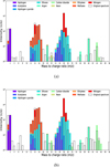 |
Fig. 2 Measured mass spectrum averaged between (a) 126-131 km and (b) 12-17 km showing the contributions of each species in different colors (mentioned in the legend) after deconvolution. The major peaks of CH4, N2, H2, and Ar seem to be well fit. The blank mass peaks are from species not considered in our calculations. |
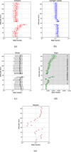 |
Fig. 3 Vertical profile of mole fractions of five trace species - (a) acetylene, (b) hydrogen cyanide, (c) ethane, (d) argon, and (e) ethylene - in their gaseous phase (plotted with their standard deviations) with a resolution of 5 km. The argon profile has been shaded above 20 km because of unreliable retrieval (Section 3.3). Mole fractions at 53 and 49 km could be unreliable, since the measurements were affected by the pump overloading due to EC experiments via Leak 3. |
3 Results
Figure 3 shows the altitudinal variation in mole fractions of five trace species (C2H2, C2H4, HCN, C2H6, and Ar) when the probe was descending through the atmosphere from an altitude of 147 km. Data has been stacked for every 5 km and points are plotted with their standard deviations (only retrieval uncertainties have been taken into account and not measurement errors). The data points from 147 km to 66 km were sampled using Leak 1 and from 55 km to the surface were sampled via Leak 2. The gas flow rate via Leak 1 was larger than via Leak 2 (CAL-PRES.DOC from NASA PDS; Team HUYGENS GCMS 2006c) as Leak 1 was open when atmospheric pressure was low. There was no atmospheric sampling between 55 and 65 km because the analysis of the EC (via L3) was taking place during that time. The function of this leak is explained in section 4.3. We found that from 1979 s (60 km), just when the EC analysis started, the remaining ions in the ion source could not be completely flushed out between consecutive mass scans. This problem persisted at least until 2683 s (46 km) and was possibly due to the sudden influx of trace gases into the ion source from EC at that instant. As a result, the getter and ion pumps connected to the ion source may have been temporarily overloaded with gas and unable to perform nominally for a few kilometers. The two data points at 53 and 49 km for all species could be due to this unprecedented situation and not related to atmospheric conditions.
3.1 Ethane and hydrogen cyanide
Ethane and hydrogen cyanide are the two most abundant hydrocarbons and nitriles, respectively, in Titan’s lower atmosphere. Ethane is the first hydrocarbon to form after methane gets dissociated by photons and energetic particles (Atreya et al. 2006). HCN is formed from the reactive radicals formed from CH4 and N2 dissociation. Titan contains the highest amount of HCN in its atmosphere amongst other bodies in the Solar System (Pearce et al. 2020). Ethane is found in the atmosphere as well as on the surface lakes, and thus is one of the prominent species that is studied on Titan. These two species are formed at higher altitudes and transported deep into the atmosphere before condensing at very low temperatures.
Figures 3b and 3c show the vertical profile of the two species as measured by the GCMS. The mole fractions of both HCN and C2H6 were constant until 80 km, after which there was an increase until 66 km (the increase was quite sharp in HCN). The mole fractions of HCN remain constant at (1.5 ± 0.7) × 10−3 in the troposphere. The high mole fractions in this species could partly be from N2 as its contribution might not have been completely removed via the cross-talk correction. On the other hand, ethane had a gradual increase from (1.2 ± 0.9) × 10−3 at 40 km to (2 ± 1.8) × 10−3 near the surface. From our analysis of the GCMS mass spectra, we derive unexpectedly high ethane and HCN mole fractions even after the probe passed through the condensation region (60-80 km).
3.2 Acetylene and ethylene
Acetylene, along with ethane, is one of the major products from the photolysis of methane in the upper atmosphere. This molecule is formed from ethane via two pathways - one is a direct formation from ethane when it reacts with C2H and photons to form C2H2, and the other is by first forming ethylene and then photodissociating it to form this molecule (Atreya et al. 2006; Vuitton et al. 2019; Dobrijevic et al. 2016). Ethylene is also a direct product of ethane but can also be formed indirectly from acetylene. These two molecules are thus interdependent. Figures 3a and 3e show the vertical profile of these species in the lower atmosphere. The mole fraction of acetylene, like HCN and C2H6, has a fairly constant profile in the stratospheric region. In the troposphere, C2H2 decreases linearly from (1.8 ± 0.9) × 10−4 at 45 km to (7 ± 4) × 10−5 at 25 km, and then is constant around 8 × 10⁻⁵ until touchdown.
The vertical profile of ethylene (Figure 3e) decreases from 5 × 10⁻⁴ at 145 km to 6.3 × 10⁻⁴ at 100 km, and then remains roughly constant until the end of the Leak 1 operation. It then decreases from 8.3 × 10⁻⁴ to 5.5 × 10⁻⁴ between 45 and 15 km, and then increases up to 6.9 × 10⁻⁴ near the surface. Only the upper limits of C2H4 are plotted because of large error bars. It is expected to be present in very low quantities quite close to the GCMS detection limit of 10−8 (Niemann et al. 2002). It shares its major peak at m/z 28 with N2, which is the most abundant species in the atmosphere. Hence, the code was unable to properly constrain this species for all simulations as it was fitting most of the m/z 28 to N2, leading to large systematic errors. Ethylene is one of the important species for understanding Titan’s chemistry, which is why we could not neglect it in our analysis.
3.3 Argon
Argon-40 is a stable isotope formed from the radioactive decay of Potassium-40. It was previously measured to be (3.39 ± 0.01) × 10−5 between 75-77 km (using the sampled Leak 3 data) and around (3.35 ± 0.25) × 10−5 from 18 km to the surface (Niemann et al. 2010). When we look at its vertical profile (Figure 3d), we see that it has a decreasing trend from (5.2 ± 1.1) × 10−4 at 145 km to (2 ± 0.5) × 10−4 at 66 km, and another decrease from (2.7 ± 0.7) × 10−4 at 40 km down to 20 km. This is unusual because Ar is inert, and hence there should be no significant variation in its profile. A probable reason could be its continuous outgassing in the ion source and the inability to completely remove this background Ar from laboratory calibrations (Niemann et al. 2010). Below 20 km, the ion source pressure must have been high enough to provide good counting statistics and estimate atmospheric mole fractions. Indeed, our retrieved profile looks constant at (1.6 ± 0.4) × 10−4, which is, however, ten times higher than that reported (the difference could be due to the unavailability of pre-flight calibrations).
4 Discussion
4.1 Comparison with other datasets and models
Except for Huygens, there had been no in situ mission in the lower atmosphere of Titan. However, the analysis of CIRS limb spectra of flyby T18 (September 7, 2006, 12°S 68°W, closest to the latitude of the Huygens landing site) allowed Vinatier et al. (2015) and Mathé et al. (2020) to infer vertical profiles of mole fractions of trace species in the stratosphere down to an altitude of 129 km. Figure 4 shows the mole fractions of C2H2, HCN, C2H4, and C2H6 retrieved in this work between 0 to 147 km (solid lines plotted with their standard deviations, C2H4 with upper limits) and data points corresponding to their mole fractions between 170 and 129 km computed using CIRS data, flyby T18 by Mathé et al. (2020) (solid lines with circular markers, 1σ std). CIRS-computed C2H4 and C2H6 mole fractions are only available down to 160 and 146 km, respectively. The ratios calculated in this paper are higher than the ones from CIRS by one (for C2H2), two (for C2H6), four (for C2H4), and five (for HCN) orders of magnitude in the stratosphere. This is a large discrepancy that could not be explained by the fact that data by CIRS and GCMS were taken at different times. Figure 5 shows a comparison between a simulated mass spectrum generated from a CIRS mixing ratio at 160 km altitude and a GCMS spectrum averaged between 130-147 km. The simulated mass spectrum was computed using the volume mixing ratios of 11 trace species reported in Mathé et al. (2020); Vinatier et al. (2015), CH4 from Lellouch et al. (2014), H2 from Courtin et al. (2012), Ar from Niemann et al. (2010), and the remaining mixing ratio was dedicated to N2. The assumptions for ionization efficiencies and fragmentation patterns used to generate this spectrum are the same as the ones we used in the deconvolution code. Both the spectra have been normalized at m/z 28. Comparing the trend of both spectra, it is clear that the C1 (12-17 u) and C2 (24-32 u) chains have similar patterns. The mass peaks of GCMS in C2 and C3 (36-46 u) chains are larger than the CIRS simulated masses. One probable reason could be the signatures of heavy species on lighter masses that are not considered here. However, the heavy species are present in very trace amounts and this big difference in spectra cannot be solely due to them. This suggests that the GCMS detected the C2 compounds considered in this paper, but their values are higher than their atmospheric composition measured by CIRS.
Fig. 4 also shows the average atmospheric composition of the four species computed from the Titan PCM model (shaded lines) at a location closest to the landing site (Lebonnois et al. 2012; de Batz de Trenquelléon et al. 2025b). The interval plots for each species represent the range of mole fractions between Ls 300° to 360°. The PCM photochemistry uses the work of Vuitton et al. (2019), which provides a more complete representation of gas cycles. There is a sharp decrease observed in the profiles of HCN, C2H2, and C2H6 below 80 km, with the HCN gaseous composition becoming negligible in the troposphere. Because most of the hydrocarbons and nitriles condense in the atmosphere at around 75 km due to low temperatures, significant trace gases are not expected to be observed below the tropopause (Lavvas et al. 2011; Wilson & Atreya 2004; de Batz de Trenquelléon et al. 2025a). From the GCMS measured mole fractions, we observe that there was no decrease in the mole fractions even as they reached their condensation temperatures (Lavvas et al. 2011; Barth 2017) and further increased for some species as the probe went down toward the surface.
Using Equation (1) in Barth (2017), condensation curves were recalculated for these four species using this paper’s volume mixing ratios (see Appendix B). If these mole fractions are actually due to atmospheric gaseous composition, then the species would condense at higher altitudes than expected. Thus, C2H6 would condense at 66.5 km instead of 63 km, C2H2 would condense at 67.5 km instead of 65.5 km, and C2H4 would condense at 64 km. But we do not see a decrease in mole fractions below these altitudes. HCN, on the other hand, with our measured volume mixing ratios, would have condensation temperatures higher than the atmospheric temperature, which means that it will be in a condensed state in the entire atmospheric range.
It is clear that, regarding trace species, the GCMS data do not match what is currently known about Titan’s lower atmospheric composition. However, the fact that the instrument still detected these species suggests that what has been measured was not solely atmospheric trace gases, contrary to what has been previously reported. We have thus identified here three potential hypotheses to interpret what the GCMS could have measured.
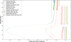 |
Fig. 4 Comparison between the mole fractions of four species calculated using our code (solid lines with 1σ std) and the one calculated using the Titan PCM model (shaded lines) from 0 to 147 km. The error bars in the PCM modeled profiles denote the range of values between Ls 300°-360°. The vertical profiles of HCN, C2H2, and C2H6 from Titan PCM show a decrease in mole fractions after condensation near the tropopause, while C2H4 does not condense in Titan conditions. Mole fractions computed using CIRS data have also been plotted at 150 km (solid lines with circular markers, 1σ std) (Mathé et al. 2020). We took results from flyby T18 for this comparison because it was conducted near the Huygens probe landing site. |
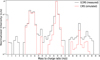 |
Fig. 5 Comparison between a simulated mass spectrum using CIRS volume mixing ratios at 160 km altitude level (red) and a GCMS mass spectrum between 130 and 147 km (black). Both mass spectra have been normalized at m/z 28. |
4.2 Hypotheses
4.2.1 Recombination inside the ion source
When a gas sample is introduced in the GCMS ion source, some molecules are fragmented into ions during the ionization process, as they interact with a strong electron beam of 70 eV. For example, a sample of 12CH4 introduced into the system could get fragmented into seven ions (H+, H2+, C+, CH+, CH2+, CH3+, CH4+), as well as neutral fragments. These ions are then electrostatically focused away from the ion source toward the mass analyzer. If these ions are not removed from the ion source to the quadrupole mass analyzer within an appropriate time and pressure range, they can recombine with other neutral gas atoms or secondary electrons to form new molecules and potentially get fragmented again (because of the continuous flow of electrons inside the ion source). The switching lens that connected the ion source to the mass analyzer was supposed to transfer the ions within microseconds (Niemann et al. 2002).
Recombination leads to the formation of new molecules that create false detections in the spectra. That is why the recombination rate should be kept to a minimum during the analysis, by maintaining a low pressure in the ion source. This can be achieved by lowering the pressure. While GCMS was not equipped with a pressure gauge in the ion source, Niemann et al. (2010) stated that for GCMS, “The maximum pressure level in the ionization region is limited by mean free path conditions to about 10−3 hPa.” If this were true, pressure in the ion source would be low enough to keep the ion-neutral recombination rate minimal (Niemann et al. 2002, 2005). If there were, however, an increase in pressure inside the ion source during the descent, it could have led to increased ion collision probabilities, which would then cause more complex ion-neutral reactions. This means that the mass spectra would carry signatures of many species that were not present in the atmosphere but were synthesized inside the ion source. However, we note that the pressure in the GCMS inlet (which had a gauge), and thus the ion source, is continually rising while descending through the atmosphere. Therefore, if this were a big effect, we would expect to see a large increase in the recombination-produced species with time of descent. Furthermore, if the trace species were formed through the reactivity of smaller more abundant species (specifically methane), we would expect a correlative decrease in this species profile as this pressure effect became more prominent at low altitudes. Since we do not see such trends, neither in trace species nor in methane profiles (Gautier et al. 2024), we can assume that recombination inside the ion source is not a likely issue for the trace gas retrieval of GCMS data.
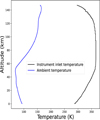 |
Fig. 6 Ambient temperature (blue) and GCMS inlet temperature (black) during the nominal science phase. |
4.2.2 Frost on the probe surface
When the probe was descending through the atmosphere, it passed through very low temperatures (100-68 K) in the stratosphere from 70 to 50 km (see Figure 6). This is the region where most gaseous species condense. It is possible that when the probe was descending through this region, some gas molecules and liquid droplets might have turned into frost on the probe surface upon contact. If frost formed all over the probe, then some ice particles could have gotten stuck at the entrance of the GCMS. These particles could then have outgassed and flowed via the heated inlet line toward the ion source. The measured spectra would thus contain contributions from outgassed particles along with atmospheric gas measurements. This hypothesis, however, could only be possible if Huygens’ exterior was not significantly warmer than the atmosphere at these altitudes. It also could not explain the high mole fractions observed above 70 km. Also, if any significant layer of frost were deposited on Huygens, it would have induced a plateau in the temperature profile measured by the HASI, which was clearly not the case (Fulchignoni et al. 2005). Hence, we can here firmly exclude this hypothesis to explain the GCMS data.
4.2.3 Aerosol and condensed particle outgassing
Figure 6 shows that when the probe was descending through the atmosphere, the temperature inside the GCMS inlet line (which is connected to the entrance of the instrument) was higher than the ambient temperature. The temperature difference was around 150-250 K for the entire altitude range. Aerosols are present in the atmosphere that formed at higher altitudes (around 1000 km) (Waite Jr et al. 2007), and transported down to lower altitudes. At very low temperatures between 40 and 80 km, most of the atmospheric gases condense out. Here, we refer to aerosols, organic material deposited on aerosols, and condensed particles collectively as ice. The heat shield that covered the GCMS inlet was released after 155 km and within 30 seconds the GCMS started sampling (Lebreton et al. 2005, 2009). It is possible that when the probe was operational the ices were carried into the GCMS sampling lines with the ambient atmosphere. Some of these could then have been stuck at the entrance, the valves, and the capillary leaks of GCMS. Figure 1 shows us a schematic diagram of the part of the GCMS connected to ion source 1 and the dotted blue circles are drawn at places where these particles could pile up during the mission. Here, we have only shown the possible locations for Leak 1 and 2 samplings, since the Leak 3 sampling does not contribute toward constructing the vertical profiles. In this scenario, it is possible that the ices could have outgassed inside the instrument due to a) the heater at the entrance, and b) the high temperature inside the instrument. Small ices could also have been evaporated while they were moving inside the instrument. Hence, what we observed from the GCMS measured spectra would not be exclusively gaseous composition but rather a mixture of gases and desorbed ices. Their contribution would not have been significant enough to alter major species (CH4 and N2) retrievals, but it definitely could impact trace gas measurements. Such a mechanism could explain why our analysis gets higher mole fractions than was measured with other instruments and model predictions. The sudden increase in Figure 3b below 80km could be due to HCN ices; however, a simultaneous pressure change due to EC at that time makes it difficult to distinguish their effect on mole fractions. While an aerosol filter on the inlet of GCMS would have prevented such a scenario, there is no record of a filter included on the GCMS atmospheric inlet in either the published instrument papers or design documentation and drawings (personal communication).
A laboratory study quantified temperatures at which different species can outgas using laboratory analogs of Titan’s aerosols (Morisson et al. 2016; He et al. 2015). It showed that lighter hydrocarbons and nitriles such as HCN, C2H4 can outgas from 200 °C. These aerosols were produced at room temperature and so the temperature difference was greater than 150 °C, similar to the difference between the ambient temperature and instrument temperature during the Huygens descent. However, additional studies on the desorption of condensed gas on aerosols at Titan relevant temperature would be needed to further the comparison.
H.B. Niemann, the Principal Investigator of Huygens GCMS, had also mentioned the possibility of GCMS measuring evaporated cloud droplets of different compounds during its operation (Niemann et al. 2002). However, due to lack of facilities to reproduce these droplets, there was no calibration done to account for this issue at the time. Because of this, it becomes very difficult to segregate these droplet measurements from the atmospheric data and we would thus not be getting the correct atmospheric composition of all species.
The third hypothesis is the one we favor to explain the GCMS data, although some discrepancies remain that we cannot fully explain. In particular, if a cloud droplet or ice entered the instrument and then sublimated, one could expect vertical variations in the signal, with the small-scale structure visible, similarly to what is observed for the methane profile (Gautier et al. 2024).
If this scenario indeed reflects what happened during Huygens’ descent toward Titan, the data sampled by the GCMS may thus contain a mixture of atmospheric gases and evaporated particles. If the hypothesis is correct, then this data could be used for further investigation on aerosol and condensed particle chemistry if we can find a way to separate their concentration from the measurements. This is quite a complicated task and it is not uncommon to find this difficulty during other space missions. The Pioneer Venus probe sampled Venusian atmospheric data from an altitude of 62 km to the surface. The neutral gas mass spectrometer could not sample between 50 and 28 km because the leaks inside the instrument were coated with sulphuric acid droplets presumed to be from clouds (Hoffman et al. 1980). Similarly, when the Philae (Rosetta mission) landed on the surface of comet 67P/Churymov-Gereismanko, it ejected a cloud of dust grains, which entered the COSAC mass spectrometer, affecting the measurements (Boehnhardt et al. 2017; Leseigneur et al. 2022). Hence, it is very important to implement methods via which particle contamination could be significantly reduced during future missions carrying a mass spectrometer on board. For example, the DAVINCI mission to Venus will implement inlets with filters and other design elements to minimize the potential impact of atmospheric particulates on the gas-phase measurements during the descent (Garvin et al. 2022).
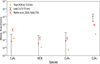 |
Fig. 7 Comparison between mole fractions calculated using Leak 3 measurements between 73 and 75 km (black triangles) and that computed using flyby T18 CIRS data between 129 km and 160 km (red circles) (Mathé et al. 2020) and Titan PCM at 73.8 km (yellow squares). |
4.3 Results from Leak 3
Apart from sampling via Leaks 1 and 2, GCMS also sampled for a limited time from 75 to 73 km via a third leak L3 (as is shown in Figure 1). The sampled gas flowed via a valve to the EC, where a majority of the hydrocarbons and nitriles were adsorbed on its surface. The remaining gas (containing nitrogen, methane, noble gases, and some other reactive gases) was removed from the cell and then moved to another cell where most reactive gases except methane were pumped out (Niemann et al. 2002, 2010). This gas (now containing methane and noble gases) was then sent to the ion source for rare gas measurements below 63 km. A few seconds later, the trace gases were desorbed from the surface of the EC, following which they mixed with the previous gas mixture for noble gas measurements and were then also measured by the spectrometer. Nitrogen was not completely removed from the system but was significantly reduced, which prevented cross-contamination at masses 26, 27, and 29.
Given that the amount of nitrogen was reduced in these measurements, it is not possible to calculate the mole fractions in a straightforward way as was done for L1 and L2 data. The species mixing ratios were retrieved by dividing their mole fraction with that of methane (calculated from L3) and then multiplying this ratio with the mole fraction of methane retrieved from L1 between 73 and 75 km. The mole fractions of four species - C2H2, C2H4, C2H6, and HCN - computed from the Leak 3 dataset were compared with the ones calculated from flyby T18 CIRS observations and the PCM model (see Figure 7). We find that the mole fraction of acetylene lies in the same range as the PCM value but is less than the CIRS values by an order of magnitude. HCN and C2H4 values from Leak 3 are quite close to the CIRS calculated values, but for C2H4 the PCM value is less by an order of magnitude. Ethane is still higher than both PCM and CIRS values, but its mole fraction is lower than what was observed in Figure 3.
The mole fractions of these four gases were found to be lower when they passed through Leak 3 than when they passed through the other two leaks. This is because sampling via this leak took place within 44 seconds for 2 km (73-75 km). Even if some aerosols did get stuck at the valves, the number of aerosols outgassing is quite less because of such a short amount of sampling time before the valve closed. This is why Figure 1 did not have possible sources marked on the L3 line. Also, should the trace species detected through L1 and L2 be due to ion source recombination, the ion source pressure would have likely been lower for L3, limiting this effect. Hence, what was observed in the spectra measured here were actual atmospheric gases and not aerosols that were observed in the entire descent spectra of Leaks 1 and 2. This is strong evidence in support of the third hypothesis made in this paper and further analysis could thus be made from this dataset to better understand the lower stratosphere of Titan.
4.4 Propane and carbon dioxide
The C3 species usually have major signatures between m/z 36 and 48. One of them is propane C3H8, which has its important peaks at m/z 29 (base peak), 43, and 44 (molecular ion peak). m/z 44 is shared also by carbon dioxide, which is not expected to be present in detectable amounts in the lower atmosphere (Niemann et al. 2010). However, we see significant peak intensities at this mass peak in Leak 1 and Leak 2 (below 20 km) measurements (see Figure 2), which could be either from propane or background CO2 (it could not be completely removed from background measurements). The mole fraction of CO2 tells us that the species was constant in the stratosphere and then started increasing below 20 km. There was a gradual increase in count rates at m/z 44 until the end of the mission, which could indicate the presence of an outgassing source of CO2 at the Huygens landing site as Niemann et al. (2010) mentioned. This means that after touchdown the major contributor at this mass peak could be evaporated carbon dioxide.
Indeed, while propane has fragments at both m/z 43 and 44, CO2 only shows a peak at m/z 44. The ratio of m/z 43/44 was constant during the descent, indicating either a sole contribution by propane, or a combination of propane and CO2 with a fixed mixing ratio. Unfortunately, it is not possible to properly quantify propane during the descent as its signal lies close to the limit of detection. On the other hand, after touchdown m/z 44 increased (Figure 8) relatively to m/z 43, which could only be due to CO2 outgassing.
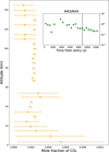 |
Fig. 8 Variation in CO2 as a function of altitude before touchdown. Some data points have been represented only with their upper limits. The figure inside is the variation in m/z 43/44 with time during the entire mission (stacked every 500 seconds). The dotted black line at 8860s is the time of probe touchdown on the surface. |
5 Conclusion
Huygens’ descent took place on January 2005 for nearly 3.5 hours, collecting data in the lower atmosphere of Titan from an altitude of 150 km. The GCMS on board this probe took nearly 1600 mass spectra by direct atmospheric sampling. In previous works done on the atmospheric portion of this data, only methane, hydrogen vertical profiles, and noble gases (7375 km) were computed. In this paper, an attempt has been made to quantify the minor gases in the atmosphere by analyzing the dataset with a new mass spectra deconvolution code (Gautier et al. 2020).
Our first finding is that the sudden sensitivity change at 73 km, which was reported by Niemann et al. (2010) as possibly being due to an ion source malfunction following parachute deployment, may actually have been caused by the propagation of a pressure wave through GCMS lines. The sensitivity drop indeed corresponds to the exact time of closing of valve VS7 (Figure 1) connected to the EC, which may have led to increased count rates for all mass peaks.
In addition, we have been able to retrieve the mole fractions of four species - C2H2, HCN, C2H4, and C2H6 - measured by GCMS. However, these mole fractions are larger than what was retrieved by remote sensing at 150 km using CIRS (Vinatier et al. 2015; Mathé et al. 2020). They are also found to be significantly larger than what was predicted by the Titan PCM in the lower atmosphere. It is expected that most trace gases in Titan’s lower atmosphere would condense out at around 75 km, after which the mole fractions would reduce significantly (Lavvas et al. 2011; Barth 2017), which was not observed in our results. Thus, it is highly likely that what this instrument measured was not just atmospheric gases.
One possible explanation for this observation, which we have explored here, is that the instrument measured condensed species in addition to atmospheric gases. These aerosols could have evaporated at certain places inside the probe (Figure 1) due to the high temperature inside the instrument as compared to the outside. Hence, the data would contain significant contributions from these particles, which could explain the high mole fractions not reflecting the actual Titan gas phase volatile inventory. The mole fractions of some species were calculated from the Leak 3 data (which was used for noble gas analyses) and matched strongly with the CIRS calculated values. This difference for L3 data may have originated in its separate sampling, done through ECs and for a very short amount of time (less than a minute), which could have minimized the aerosol contamination. Hence, mole fractions retrieved from Leak 3 are actual atmospheric gas measurements and these are by far the only trace gas measurements in the lower atmosphere of Titan.
If it is possible that GCMS may have sampled the volatiles emitted from aerosols upon heating, it would be useful to compare these results with the ones from the Aerosols Collector and Pyrolyzer (ACP) on the probe. This instrument was used to collect aerosols, pyrolyze them in an oven, and send the gaseous products to one of the ion sources of GCMS to measure the composition of the evolved gas. Previous work on this data was able to identify NH3 and HCN when the samples were heated up to 600°C, which could mean that these two species are present within the refractory core of aerosols (Israël et al. 2005). On the other hand, the heating of aerosols within GCMS itself would have occurred at around 100°C. As was mentioned above, at these temperatures we observed a significant amount of HCN at all altitudes.
On the other hand, NH3 could not be identified in the GCMS data from our results. In fact, the ratio between m/z 16 and 17 was nearly constant throughout the descent, and consistent with the expected ratio due to the 12C/13C isotopic ratio in CH4 determined from CIRS (Nixon et al. 2008). He et al. (2015) showed from laboratory experiments that ammonia is released from the Titan aerosols analogs starting from 200 ° C. This could be the reason why we do not observe this species at lower temperatures as it was not sufficient to break down the aerosols. Since we observe HCN at relatively low heating, we may hypothesize that the nitriles observed were a condensed layer on the aerosols rather than incorporated in the aerosol macromolecules. Only the much more energetic heating of ACP at 600 °C was sufficient to volatilize these nitrogen-bearing groups in the form of ammonia. ACP also performed measurements at ambient temperature and 250 °C, the results of which could help us to further investigate this hypothesis, but detailed investigations on these data are yet to be done.
Our work suggests that the GCMS may have measured aerosols and condensed particles (near tropopause) throughout its operational phase. Though we may be sensing evaporation of some ices, the pressure and CH4/N2 measurements do not indicate a clog, and so the primary measurements were not compromised. Even if a quantitative analysis would be difficult, as it is hard to segregate between atmospheric and aerosol species from the mass spectra without prior calibrations, the GCMS dataset could prove to be an useful dataset to further investigate the volatiles present in Titan’s atmosphere as probed during the descent.
Acknowledgements
We thank the NASA Planetary Data System for making the GCMS dataset public for us to use in our research. We are grateful to ANR and PNP for funding this research- ANR-20-CE49-0004-01 to K. Das, T. Gautier and M. Coutelier, CDAP162-0087 to T. Gautier, M.G. Trainer and S.M. Hörst, CDAP80NSSC19K0903 to J. Serigano and S.M. Hörst, Flare workpackage to M.G. Trainer. A special thanks to Marcello Fulchignoni (Professor at Université Paris Diderot Paris 7), P.I. of HUygens-HASI, for fruitful discussions and his input on the second hypothesis. Lastly, we are immensely grateful to Dr. Melissa G. Trainer (NASA Goddard Space Flight Center) for her valuable feedback and suggestions on the findings of this paper.
Appendix A Calculating cross-talk of mass peaks
The GCMS took eight fractional mass scans (least count of 0.125u) between m/z 18 and 35.5 during the mission. These mass scans were first corrected for raw counts, saturation at m/z 28, and background removal (mentioned in the Data treatment section) and then averaged. The averaged spectra (red, Figure A.1) was then introduced to a software called FitYK (Wojdyr 2010) which is useful for manually fitting different functions to a dataset. Since m/z 28 seemed to have a left-tailed distribution, left-tailed lognormal distribution curves were fit for masses 27, 28, 29 and 30. Figure A.1 shows the best possible combination of the four fit curves such that it matches the closest to the measured signal. Upon finding the best fit, we removed all distributions except the one at m/z 28 to find its contribution at other masses. Here we are only concerned with the intensities/measurements at whole masses since the data used to calculate vertical profiles are not fractional masses. Ratios between the remaining intensities (by subtracting fit m/z 28 value from each peak) and original intensities at masses 26, 27, 29 were calculated. These ratios were then multiplied with the measured peak values at all altitudes. The contribution of m/z 28 at 29 was found negligible. The corrected measurements are now expected to be solely due to their respective mass-to-charge ions and can be taken for further analysis. However, we must keep in mind that this is an empirical method to remove cross-talk so it is possible that there could still be contamination (lesser though) from m/z 28.
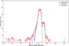 |
Fig. A.1 Averaged fractional mass scan (red) measured by Leak 2. The combination curve of the fit lognormal distribution at masses 26, 27, 28 and 29 is shown by a blue line. A left-tailed lognormal distribution was fit at mass 28 (green) to see its contribution at the neighboring mass peaks. |
Appendix B Condensation levels
The condensation temperatures of C2H2, C2H4, C2H6, and HCN has been computed from Equation (1) in Barth (2017). We calculated the altitudes at which these species would condense if their atmospheric composition were similar to the GCMS-measured mole fractions by extrapolating condensation curves from Barth (2017). The figure below shows the Barth (2017) (solid lines) and new (dashed lines) condensation curves in the lower atmosphere. The species will condense at the altitude where the condensation curves intersect with the atmospheric temperature profile (measured by HASI on the Huygens probe). The vapor pressures were calculated from coefficients available in the CHERIC database.
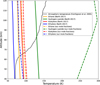 |
Fig. B.1 Vertical profiles of condensation curves of four species- C2H2, C2H4, C2H6, HCN calculated in Barth (2017) (solid lines) and by using the mole fractions derived from this paper (dashed lines). The black line is the atmospheric temperature profile measured by Huygens HASI. |
References
- Atreya, S. K., Adams, E. Y., Niemann, H. B., et al. 2006, Planet. Space Sci., 54, 1177 [NASA ADS] [CrossRef] [Google Scholar]
- Barth, E. L. 2017, Planet. Space Sci., 137, 20 [NASA ADS] [CrossRef] [Google Scholar]
- Boehnhardt, H., Bibring, J.-P., Apathy, I., et al. 2017, Philos. Trans. Roy. Soc. A: Math. Phys. Eng. Sci., 375, 20160248 [Google Scholar]
- Clausen, K. C., Hassan, H., Verdant, M., et al. 2002, Space Sci. Rev., 104, 155 [Google Scholar]
- Coates, A. J., Crary, F. J., Lewis, G. R., et al. 2007, Geophys. Res. Lett., 34 [Google Scholar]
- Courtin, R., Sim, C. K., Kim, S. J., & Gautier, D. 2012, Planet. Space Sci., 69, 89 [Google Scholar]
- de Batz de Trenquelléon, B., Rannou, P., Burgalat, J., Lebonnois, S., & Vatant d’Ollone, J. 2025a, Planet. Sci. J. [Google Scholar]
- de Batz de Trenquelléon, B., Rosset, L., Vatant d’Ollone, J., et al. 2025b, Planet. Sci. J. [Google Scholar]
- Dobrijevic, M., Loison, J., Hickson, K., & Gronoff, G. 2016, Icarus, 268, 313 [NASA ADS] [CrossRef] [Google Scholar]
- Fulchignoni, M., Ferri, F., Angrilli, F., et al. 2002, Space Sci. Rev., 104, 395 [Google Scholar]
- Fulchignoni, M., Ferri, F., Angrilli, F., et al. 2005, Nature, 438, 785 [CrossRef] [Google Scholar]
- Galand, M., Yelle, R. V., Coates, A. J., Backes, H., & Wahlund, J. E. 2006, Geophys. Res. Lett., 33 [Google Scholar]
- Garvin, J. B., Getty, S. A., Arney, G. N., et al. 2022, Planet. Sci. J. 3, 117 [NASA ADS] [CrossRef] [Google Scholar]
- Gautier, T., Serigano, J., Bourgalais, J., Hörst, S. M., & Trainer, M. G. 2020, Rapid Commun. Mass Spectrom., 34, e8684 RCM-19-0297.R1 [Google Scholar]
- Gautier, T., Serigano, J., Das, K., et al. 2024, A&A, 690, A165 [NASA ADS] [CrossRef] [EDP Sciences] [Google Scholar]
- He, J., Buch, A., Carrasco, N., & Szopa, C. 2015, Icarus, 248, 205 [Google Scholar]
- Hoffman, J., Hodges, R., Donahue, T., & McElroy, M. 1980, J. Geophys. Res.: Space Phys., 85, 7882 [Google Scholar]
- Hörst, S. M. 2017, J. Geophys. Res. (Planets), 122, 432 [Google Scholar]
- Hunten, D. M. 1978, JPL The Saturn System [Google Scholar]
- Hwang, W., Kim, Y.-K., & Rudd, M. E. 1996, J. Chem. Phys., 104, 2956 [NASA ADS] [CrossRef] [Google Scholar]
- Israël, G., Szopa, C., Raulin, F., et al. 2005, Nature, 438, 796 [CrossRef] [Google Scholar]
- Kim, Y.-K., & Rudd, M. E. 1994, Phys. Rev. A, 50, 3954 [NASA ADS] [CrossRef] [Google Scholar]
- Kim, Y.-K., Ali, M. A., & Rudd, M. E. 1997a, J. Res. Natl. Inst. Standards Technol., 102, 693 [Google Scholar]
- Kim, Y.-K., Hwang, W., Weinberger, N., Ali, M., & Rudd, M. E. 1997b, J. Chem. Phys., 106, 1026 [NASA ADS] [CrossRef] [Google Scholar]
- Lavvas, P., Griffith, C. A., & Yelle, R. V. 2011, Icarus, 215, 732 [NASA ADS] [CrossRef] [Google Scholar]
- Lebonnois, S., Burgalat, J., Rannou, P., & Charnay, B. 2012, Icarus, 218, 707 [CrossRef] [Google Scholar]
- Lebreton, J.-P. 2018, in EGU General Assembly Conference Abstracts, 18695 [Google Scholar]
- Lebreton, J.-P., & Matson, D. 2002, Space Sci. Rev., 104, 59 [Google Scholar]
- Lebreton, J.-P., Witasse, O., Sollazzo, C., et al. 2005, Nature, 438, 758 [Google Scholar]
- Lebreton, J.-P., Coustenis, A., Lunine, J., et al. 2009, A&A Rev., 17, 149 [Google Scholar]
- Lellouch, E., Bézard, B., Flasar, F., et al. 2014, Icarus, 231, 323 [CrossRef] [Google Scholar]
- Leseigneur, G., Bredehöft, J. H., Gautier, T., et al. 2022, Angew. Chem. Int. Ed., 61, e202201925 [Google Scholar]
- Lunine, J. I., & Atreya, S. K. 2008, Nat. Geosci., 1, 159 [NASA ADS] [CrossRef] [Google Scholar]
- Mathé, C., Vinatier, S., Bézard, B., et al. 2020, Icarus, 344, 113547 [CrossRef] [Google Scholar]
- Morisson, M., Szopa, C., Carrasco, N., Buch, A., & Gautier, T. 2016, Icarus, 277, 442 [Google Scholar]
- Niemann, H. B., Atreya, S. K., Bauer, S. J., et al. 2002, Space Sci. Rev., 104, 553 [CrossRef] [Google Scholar]
- Niemann, H. B., Atreya, S. K., Bauer, S. J., et al. 2005, Nature, 438, 779 [Google Scholar]
- Niemann, H. B., Atreya, S. K., Demick, J. E., et al. 2010, J. Geophys. Res. (Planets), 115, E12006 [CrossRef] [Google Scholar]
- Nixon, C. A. 2024, ACS Earth Space Chem., 8, 406 [NASA ADS] [CrossRef] [Google Scholar]
- Nixon, C. A., Achterberg, R. K., Vinatier, S., et al. 2008, Icarus, 195, 778 [Google Scholar]
- Pearce, B. K., Molaverdikhani, K., Pudritz, R. E., Henning, T., & Hébrard, E. 2020, ApJ, 901, 110 [NASA ADS] [CrossRef] [Google Scholar]
- Porco, C. C., Baker, E., Barbara, J., et al. 2005, Nature, 434, 159 [NASA ADS] [CrossRef] [Google Scholar]
- Robertson, I., Cravens, T., Waite, J., et al. 2009, Planet. Space Sci., 57, 1834 [NASA ADS] [CrossRef] [Google Scholar]
- Serigano, J., Hörst, S. M., He, C., et al. 2020, J. Geophys. Res. (Planets), 125, e06427 [Google Scholar]
- Serigano, J., Hörst, S. M., He, C., et al. 2022, J. Geophys. Res.: Planets, 127, e2022JE007238 [Google Scholar]
- Team HUYGENS GCMS 2006a, DATA Processing, nASA Planetary Data System [Google Scholar]
- Team HUYGENS GCMS 2006b, DESC_FM_08F, nASA Planetary Data System [Google Scholar]
- Team HUYGENS GCMS 2006c, Prelaunch calibration file [Google Scholar]
- Vinatier, S., Bézard, B., Lebonnois, S., et al. 2015, Icarus, 250, 95 [NASA ADS] [CrossRef] [Google Scholar]
- Vuitton, V., Yelle, R. V., Klippenstein, S. J., Hörst, S. M., & Lavvas, P. 2019, Icarus, 324, 120 [CrossRef] [Google Scholar]
- Waite, J., Kasprzak, W., Luhman, J., et al. 2018, Cassini INMS level 1A data archive, nASA Planetary Data System [Google Scholar]
- Waite Jr, J., Young, D., Cravens, T., et al. 2007, Science, 316, 870 [CrossRef] [Google Scholar]
- Wilson, E. H., & Atreya, S. K. 2004, J. Geophys. Res.: Planets, 109 [Google Scholar]
- Wojdyr, M. 2010, J. Appl. Crystallogr., 43, 1126 [CrossRef] [Google Scholar]
All Figures
|
Fig. 1 Schematic diagram of gas flow inside the GCMS through ion source 1. The eight blue hexagons and three red cylinders are the valves and leaks, respectively, and they have been labeled similarly to the instrument diagram in Niemann et al. (2002) paper. Gas flows through L1, L2, and L3 at different times during the mission. The valves were used for specific purposes and their functions are mentioned in Niemann et al. (2002). Dotted blue circles represent the possible sources of aerosol accumulation in the GCMS (explained in Section 4.2.3) |
| In the text | |
|
Fig. 2 Measured mass spectrum averaged between (a) 126-131 km and (b) 12-17 km showing the contributions of each species in different colors (mentioned in the legend) after deconvolution. The major peaks of CH4, N2, H2, and Ar seem to be well fit. The blank mass peaks are from species not considered in our calculations. |
| In the text | |
|
Fig. 3 Vertical profile of mole fractions of five trace species - (a) acetylene, (b) hydrogen cyanide, (c) ethane, (d) argon, and (e) ethylene - in their gaseous phase (plotted with their standard deviations) with a resolution of 5 km. The argon profile has been shaded above 20 km because of unreliable retrieval (Section 3.3). Mole fractions at 53 and 49 km could be unreliable, since the measurements were affected by the pump overloading due to EC experiments via Leak 3. |
| In the text | |
|
Fig. 4 Comparison between the mole fractions of four species calculated using our code (solid lines with 1σ std) and the one calculated using the Titan PCM model (shaded lines) from 0 to 147 km. The error bars in the PCM modeled profiles denote the range of values between Ls 300°-360°. The vertical profiles of HCN, C2H2, and C2H6 from Titan PCM show a decrease in mole fractions after condensation near the tropopause, while C2H4 does not condense in Titan conditions. Mole fractions computed using CIRS data have also been plotted at 150 km (solid lines with circular markers, 1σ std) (Mathé et al. 2020). We took results from flyby T18 for this comparison because it was conducted near the Huygens probe landing site. |
| In the text | |
|
Fig. 5 Comparison between a simulated mass spectrum using CIRS volume mixing ratios at 160 km altitude level (red) and a GCMS mass spectrum between 130 and 147 km (black). Both mass spectra have been normalized at m/z 28. |
| In the text | |
|
Fig. 6 Ambient temperature (blue) and GCMS inlet temperature (black) during the nominal science phase. |
| In the text | |
|
Fig. 7 Comparison between mole fractions calculated using Leak 3 measurements between 73 and 75 km (black triangles) and that computed using flyby T18 CIRS data between 129 km and 160 km (red circles) (Mathé et al. 2020) and Titan PCM at 73.8 km (yellow squares). |
| In the text | |
|
Fig. 8 Variation in CO2 as a function of altitude before touchdown. Some data points have been represented only with their upper limits. The figure inside is the variation in m/z 43/44 with time during the entire mission (stacked every 500 seconds). The dotted black line at 8860s is the time of probe touchdown on the surface. |
| In the text | |
|
Fig. A.1 Averaged fractional mass scan (red) measured by Leak 2. The combination curve of the fit lognormal distribution at masses 26, 27, 28 and 29 is shown by a blue line. A left-tailed lognormal distribution was fit at mass 28 (green) to see its contribution at the neighboring mass peaks. |
| In the text | |
|
Fig. B.1 Vertical profiles of condensation curves of four species- C2H2, C2H4, C2H6, HCN calculated in Barth (2017) (solid lines) and by using the mole fractions derived from this paper (dashed lines). The black line is the atmospheric temperature profile measured by Huygens HASI. |
| In the text | |
Current usage metrics show cumulative count of Article Views (full-text article views including HTML views, PDF and ePub downloads, according to the available data) and Abstracts Views on Vision4Press platform.
Data correspond to usage on the plateform after 2015. The current usage metrics is available 48-96 hours after online publication and is updated daily on week days.
Initial download of the metrics may take a while.