| Issue |
A&A
Volume 700, August 2025
|
|
|---|---|---|
| Article Number | A194 | |
| Number of page(s) | 16 | |
| Section | Interstellar and circumstellar matter | |
| DOI | https://doi.org/10.1051/0004-6361/202553948 | |
| Published online | 19 August 2025 | |
Deep survey of millimeter radio recombination lines toward the planetary nebulae IC 418 and NGC 7027
1
Instituto de Astrofísica de Canarias (IAC),
C/ Vía Láctea s/n,
38205
La Laguna,
Spain
2
Departamento de Astrofísica, Universidad de La Laguna (ULL),
38206
La Laguna,
Spain
3
Observatorio Astronόmico Nacional (OAN, IGN/CNIG),
C/ Alfonso XII3,
28014
Madrid,
Spain
4
Department of Space, Earth and Environment, Chalmers University of Technology, Onsala Space Observatory,
439 92
Onsala,
Sweden
5
Departamento de Astrofísica Molecular, Instituto de Física Fundamental (IFF, CSIC),
C/ Serrano 123,
28006
Madrid,
Spain
6
Consejo Superior de Investigaciones Científicas (CSIC),
Spain
7
Departament de Física Quàntica i Astrofísica (FQA), Universitat de Barcelona (UB),
C/ Martí i Franqués 1,
08028
Barcelona,
Spain
8
Institut de Ciències del Cosmos (ICCUB), Universitat de Barcelona (UB),
C/ Martí i Franqués 1,
08028
Barcelona,
Spain
★ Corresponding author: This email address is being protected from spambots. You need JavaScript enabled to view it.
Received:
29
January
2025
Accepted:
28
June
2025
Abstract
Context. The circumstellar environments of planetary nebulae (PNe) are remarkably chemically rich astrophysical laboratories, proving useful for studies of the ionization of atoms and the formation of simple and complex molecules. The new generation of high-sensitivity receivers opens up the possibility to carry out the deep observations needed to unveil the weak atomic and molecular spectra lying in the millimeter (mm) range.
Aims. The main goal of this work is to study the emission lines detected in the spectra of the bright C-rich PNe IC 418 and NGC 7027 and to identify all those emission features associated with the radio recombination lines (RRLs) of light elements. We aim to analyze the RRLs detected for each source, model the sources, and derive their physical parameters. This work has allowed us to provide the most complete and updated catalog of RRLs in space.
Methods. We present the results of our very deep line survey of IC 418 and NGC 7027 carried out at 2, 3, and 7 mm with the IRAM 30m and the Yebes 40m radio telescopes. We compared these observational data sets with synthetic models produced with the radiation transfer code Co3RaL.
Results. Our observations toward the target PNe reveal the presence of several H and He I RRLs at mm wavelengths in the spectra of IC 418 and NGC 7027 and also of He II RRLs in the spectrum of NGC 7027. Many of these lines had remained undetected until now due to their weakness and the lack of high-sensitivity observations at these frequencies. The data also confirm the absence of molecular emission toward IC 418, above a detection level of ~3 mK [Tmb].
Conclusions. These mm observations represent the most extended RRL line survey of two C-rich PNe carried out thus far, with most of the lines reported for the first time. These extremely complete catalogs evidence the importance of high-sensitivity observations and are expected to be very helpful in the line identification process in mm observations, particularly for molecular species in the vicinity of ionized environments that are still unknown or poorly characterized.
Key words: catalogs / radio lines: stars / submillimeter: stars / planetary nebulae: individual: IC 418 / planetary nebulae: individual: NGC 7027
© The Authors 2025
 Open Access article, published by EDP Sciences, under the terms of the Creative Commons Attribution License (https://creativecommons.org/licenses/by/4.0), which permits unrestricted use, distribution, and reproduction in any medium, provided the original work is properly cited.
This article is published in open access under the Subscribe to Open model. This email address is being protected from spambots. You need JavaScript enabled to view it. to support open access publication.
1 Introduction
The planetary nebula (PN) phase is the last stage in the evolution of the circumstellar envelope (CSE) around a star with initial mass of ~ 1–8 M⊙. During the preceding asymptotic giant branch (AGB; see e.g., Herwig 2005, for a review), the star experiences a series of thermal pulses (or periodic He-shell flashes). This favors the nucleosynthesis of both light and heavy neutron-rich chemical elements (Karakas & Lattanzio 2014). Such newly synthesized chemical elements are mixed from the H-burning shell to the stellar surface via several third dredge-up events (TDUs). During each TDU, the C from the core is driven to the stellar surface, increasing its C/O ratio.
Throughout the AGB phase, stars also experience strong mass loss (up to ~10–4 M⊙ a–1) caused by a stellar wind originating in the envelope. The process of mass loss produces a CSE around the central star that expands and efficiently enriches the interstellar medium (ISM) with atomic and molecular gas and dust grains (Tielens 2005; Tielens et al. 2005). When this process abruptly stops, the star increases its effective temperature (Teff), entering into a short-lived (~102–104 a) post-AGB stage (see e.g., García-Lario 2006) toward the formation of a white dwarf. A PN emerges when the central star is hot enough (Teff ≥ 30 000 K) to photoionize the surrounding circumstellar material expelled during the preceding AGB phase.
The low-mass (~ 1.5–3.5 M⊙) stars are converted to C-rich (C/O > 1 at the stellar surface) by the end of the AGB phase, forming a C-rich CSE that provides a fantastic laboratory to detect C-based species. The detection of organic species in these environments provides invaluable insights to understand the complexity of the organic chemistry in space (see e.g., Kwok 2016; Pardo et al. 2022; Cabezas et al. 2023; Cernicharo et al. 2023; Pardo et al. 2023; Gupta et al. 2024, and references therein). Indeed, an important number of organic molecules have been detected toward the nearby and bright (prototypical) C-rich AGB star IRC +10216 via their rotational lines in the radio domain (see e.g., Agúndez et al. 2014; Cernicharo et al. 2017, 2019; McGuire 2022; Tuo et al. 2024; Cernicharo et al. 2024a, and references therein).
In the subsequent PN phase, the hot central star emits very energetic UV photons, creating an environment that favors chemical reactions: simple and complex molecules coexist with radicals, ions, and atoms under extreme and rapidly changing conditions. However, even though the current list of molecules detected in PNe is significant (see e.g., Bublitz et al. 2019; Schmidt et al. 2022), the exact chemical pathways necessary to produce each species remain unclear. In particular, the largest organic molecules detected to date, such as C60 and C70 fullerenes (Cami et al. 2010; García-Hernádez et al. 2010), are formed in (proto-) PNe through processes that are still under debate (see e.g., Gόmez-Muñoz et al. 2024, and references therein).
To drive the field forward, more molecular species (specifically, the key molecular by-products or precursors) need to be detected in the radio domain. Such key possible molecular species may have remained undetected because of their weak rotational lines and the lack of accurate laboratory and theoretical spectroscopic information. The weakness of a rotational line might be due to several factors such as the low molecular abundance or low dipolar moments, but the size of the molecule is fundamental. The larger the molecule, the higher the number of rotational levels. This also implies a large rotational partition function even at low temperatures, and, consequently, low populated rotational levels. Therefore, the rotational lines associated with large C-based molecules are intrinsically weak. In this context, deep radio observations, which use very large antennas and long exposure times, are essential to detect the weak rotational lines of the possible key molecular species. The significant noise reduction in deep radio observations may thus reveal new weak features, from both molecules and atoms, which have remained undetected to date.
In the ionized PN, many radio emission lines associated with atoms and molecules can be observed. Their radio spectra can also display emission due to new molecules in space that may remain mislaid among known molecular lines and atomic lines. This is particularly true for radio recombination lines (RRLs)1 and, therefore, the detection and identification of the numerous atomic RRLs is a crucial task in identifying the spectra of new molecular species. The RRLs mainly originate in the ionized hydrogen rich region around the central star of the PN. However, it ought to be noted here that C I RRLs predominantly originate from the neutral hydrogen regions surrounding the PN. RRLs are not affected by dust opacity, so they turn out to be a precise tool to determine the electron temperature, Te, and density, ne, but also to analyze the relative abundance of He to H or to determine the kinematic distance to the H II region (see Mezger & Palmer 1968, and references therein). The latter has been a very useful technique during the early stages of radio astronomy to study the large-scale distribution of H II regions in the Galaxy (see e.g., Mezger & Hoglund 1967; Dieter 1967). Another consequence (and, thus, application) of the study of RRLs is the development of precise numerical methods to derive and calculate the Einstein coefficients characterizing the absorption and emission processes for each observed line (see e.g., Kardashev 1959; Brocklehurst 1970, 1971; Hummer & Storey 1987, 1992; Storey & Hummer 1988, 1995, and references therein for a complete overview of this complex numerical problem).
The observed RRLs have been detected toward diverse astro-physical objects like H II regions and infrared (IR) dark clouds, among others; however, PNe, emitting photons energetic enough to ionize light elements H, He, C, and O, provide an ideal astro-physical environment to produce them. Previous studies have reported the detection of several molecular lines and RRLs in very bright PNe such as those addressed in this work, IC 418 and NGC 7027 (see e.g., Goldberg 1970; Bignell 1974; Churchwell et al. 1976; Chaisson & Malkan 1976; Walmsley et al. 1981; Garay et al. 1989; Roelfsema et al. 1991; Zhang et al. 2008). These works have aimed to characterize the chemical environment of those objects with the radio astronomy facilities available; namely, to detect molecular lines or to analyze the spatial distribution of the molecular and atomic emission across the nebula. These works used RRLs toward those sources to determine a number of physical parameters. However, the sensitivities achieved in those works (≥8 mK ![Mathematical equation: $\left[ {T_{\rm{a}}^*} \right]$](/articles/aa/full_html/2025/08/aa53948-25/aa53948-25-eq1.png) ) are low compared with the sensitivities typically obtained nowadays. Current receivers can provide higher sensitivities in the objects of interest (specifically, IC 418 and NGC 7027) and detect atomic and molecular lines that had previously gone unnoticed. Indeed, no RRLs weaker than Hnδ and He I nγ2 toward our sample of sources (see e.g., Zhang et al. 2008; Guzman-Ramirez et al. 2016) had been observed because of the prior limited sensitivity.
) are low compared with the sensitivities typically obtained nowadays. Current receivers can provide higher sensitivities in the objects of interest (specifically, IC 418 and NGC 7027) and detect atomic and molecular lines that had previously gone unnoticed. Indeed, no RRLs weaker than Hnδ and He I nγ2 toward our sample of sources (see e.g., Zhang et al. 2008; Guzman-Ramirez et al. 2016) had been observed because of the prior limited sensitivity.
In this paper, we present high-sensitivity (~1 mK ![Mathematical equation: $\left[ {T_{\rm{a}}^*} \right]$](/articles/aa/full_html/2025/08/aa53948-25/aa53948-25-eq2.png) ) single-dish observations of H and He RRLs at 2, 3, and 7 mm toward the bright PNe IC 418 and NGC 7027. These two PNe are proto-typical sources displaying different properties (such as, presence of C60), geometries, and evolutionary stages. By comparing them, we may obtain key insights on possible chemical pathways as well as their atomic and molecular content as well as its influence, along with geometry, on the evolution of the PN. In Section 2, we present the radio observations and the corresponding high-sensitivity data obtained. The procedure for the identification and modeling of the RRLs is presented in Section 3. The RRLs catalogs for each PN are presented in Sections 4 and 5, together with the identification and modeling of the detected RRLs. Present and future possible applications and utilities of the RRLs catalogs are briefly discussed in Section 6. Finally, the conclusions of our work are summarized in Section 7.
) single-dish observations of H and He RRLs at 2, 3, and 7 mm toward the bright PNe IC 418 and NGC 7027. These two PNe are proto-typical sources displaying different properties (such as, presence of C60), geometries, and evolutionary stages. By comparing them, we may obtain key insights on possible chemical pathways as well as their atomic and molecular content as well as its influence, along with geometry, on the evolution of the PN. In Section 2, we present the radio observations and the corresponding high-sensitivity data obtained. The procedure for the identification and modeling of the RRLs is presented in Section 3. The RRLs catalogs for each PN are presented in Sections 4 and 5, together with the identification and modeling of the detected RRLs. Present and future possible applications and utilities of the RRLs catalogs are briefly discussed in Section 6. Finally, the conclusions of our work are summarized in Section 7.
2 Observations and data reduction
The spectra of both PNe were obtained with the IRAM 30m and Yebes 40m radio telescopes. The 30m telescope is located at 2850 m on the Pico Veleta in Sierra Nevada (Granada, Spain) and it is operated by the Institut de Radioastronomie Millimétrique3. The observations were carried out during the 2021–2022 winter semester (proposal ID 158-21) using the Eight MIxer super-heterodyne Receiver (EMIR4, Carter et al. 2012). This receiver simultaneously provides an observing bandwidth of up to 32 GHz. We performed the observations in the dual-band (E090 and E130 receivers at 3 mm and 2 mm, respectively) single-sideband (LSB) dual-polarization mode (H+V). This setup allowed us to simultaneously cover two 8 GHz wide frequency ranges (81 to 89 GHz with the E090 and 131 to 139 GHz with the E130) in both polarizations.
The spectrometer used in this project was the fast Fourier transform (FFT) to sample the whole 32 GHz observed range (that is, two receivers × two polarizations × 8 GHz). The FFT was used in the 200 kHz mode, which is equivalent to a resolution in velocity units of ~0.43 km s–1 and ~0.67 km s–1 at 2 and 3 mm, respectively. We improved the signal-to-noise ratio (SNR) of the 3 mm spectrum by smoothing to a final velocity resolution of ~1.3 km s–1. We calibrated the observations following the standard procedure at the 30m telescope. We first observed hot and cold loads (at room and liquid nitrogen temperature) to scale the spectrometer units into temperature units. Then, we observed the blank sky every 20 min in the observing session to measure the transmission properties of the local atmosphere. The backend provides the final data in (atmosphere-corrected) antenna temperature  . The absolute calibration accuracy is ~10% at 2 and 3 mm. After finishing the observations, we compared the continuum emission of every session. The measurements are stable throughout all the days, so the relative calibration between the two mm bands is good.
We observed the sources using the wobbler switching mode (WSW), which consists on nodding the sub-reflector between ON-source and OFF-source positions with a nodding frequency of 0.5 Hz. The OFF-position has to be larger than the beam size at each frequency band, so we used a separation of ±60 arcsec in azimuth with respect to each target. The WSW mode guarantees an accurate removal of instrumental and atmospheric signal, providing very flat baselines. However, the strong continuum emission of our sources left a rippled baseline after the OFF-source position subtraction (see more information at the end of this section). Despite the good pointing of the telescope, with typical errors of about 2–4 arcsec, we observed strong continuum sources located very close to the targets in the sky to ensure that the pointing of the antenna was correct. This checking procedure was done every two hours or when a new target is selected. We used one of our sources, NGC 7027, as flux calibrator due to its high brightness. The total time spent on these observations were 42 and 23 hours for IC 418 and NGC 7027, respectively.
We decided to change the frequency of the local oscillator (LO) during the observations by 100 MHz. This strategy allows us to ensure that the detected signals come from the sky and are not due to local origin (parasites or interferences). Any signal from the source will appear in the spectrum at the same frequency position, independently of the frequency of the LO. However, signals produced elsewhere appear displaced depending on the frequency of the LO. This is an optimal procedure to locate radio frequency interferences (RFI) or signals with an undesired origin. We observed half of the total project time with each LO frequency.
The Yebes 40 m antenna (RT40m)5 is located at 980 m in the Centro Astronόmico de Yebes (Guadalajara, Spain). This facility is operated by the Spanish Instituto Geográfico Nacional (IGN, Ministerio de Transportes y Movilidad Sostenible – MTMS). The observations took place during the 2021/2022 winter semester (proposal ID 22A011) using the Q-band receiver. This receiver allows us to simultaneously observe a bandwidth of 18.5 GHz with a spectral coverage of 31.5–50 GHz distributed in eight sub-bands. We carried out the observations in the dual polarization mode (H+V).
The backends used were the FFTs, that provide a resolution of 38 kHz for a bandwidth of 2.5 GHz. To cover the whole Q-band, we used eight sub-bands, whose resolution is equivalent to ~0.35–0.26 km s–1 from the first to the last sub-band. We smoothed the spectra of each sub-band to a final frequency resolution of ~300 kHz (~2.8–1.8 km s–1) to improve the SNR. The standard calibration procedure at the RT40m is similar to the procedure in the 30m and the absolute calibration accuracy is 10–15%. We observed hot and cold loads to scale to temperature units. We checked the goodness of this absolute calibration by observing the continuum emission of one of the science targets, NGC 7027, and ensuring that is was roughly constant over the observing sessions.
The observations were performed using the position switching mode (PSW), which consists of moving the telescope between the ON-source and OFF-source positions. We selected an OFF-position with an offset of 400 arcsec in horizontal direction away from the target. The PSW mode provides quite flat baselines after subtracting the OFF-position integrations. However, the final spectra show a rippled structure as in the 30m (see more information at the end of this section). Pointing and focus are good on the RT40 m, but were checked every 1.5 h with Orion IRC2 to make corrections if necessary. The PNe IC 418 and NGC 7027 were observed during 69 and 11 hours, respectively. We used the same strategy to identify RFI as in the 30 m telescope.
The data were reduced using the Continuum and Line Analysis Single-dish Software (CLASS) program of the GILDAS6 astronomical software package (sept22a version). We first inspected the data to flag bad scans and channels and average the valid data. We checked the presence of RFI by comparing the average of each polarization for each observing session at each LO frequency, the average of both polarizations for each observing session at each LO frequency, total average of each polarization at each LO frequency, and average of both polarizations at each LO frequency.
The spectra of both sources measured with each telescope were rescaled to main-beam temperature (Tmb) using
 (1)
(1)
where ηf and ηmb are the forward and main beam efficiencies, respectively. We followed the procedure detailed for the 30m7 and the RT40m. We also provide the efficiencies used for each telescope at each frequency and polarization on Table 1.
As we mentioned above, IC 418 and NGC 7027 display very strong continuum emission that produced a rippled final spectra, even though the WSW and the PSW usually provide very flat baselines. The width of these ripples is significantly larger than the width of the emission lines, so we could carefully remove it without modifying the shapes and intensities of real weak emission lines. The process consisted on slicing the spectra in small intervals (~200 MHz) and subtracting their baselines using low-degree polynomials (from zero to fourth order). Later, we stitched the flattened spectral segments to obtain a final flat and ripple-corrected spectrum for each source and frequency range. Examples of these final spectra are shown in Fig. 1.
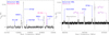 |
Fig. 1 Examples of the RT40m spectrum of IC 418 (left) and the IRAM 30 m spectrum of NGC 7027 (right). The gray arrow on the right panel indicates an absorption feature produced by some molecule in the line of sight of NGC 7027 (probably from a cold shell of its molecular envelope). |
Forward and beam efficiencies of the RT40 m and IRAM 30 m in 2022.
3 Identification, fitting, and modeling of RRLs
3.1 Identification and fitting of RRLs
Preliminary identification of the RRLs detected in our sample PNe was made by calculating the theoretical frequencies and comparing them with the frequencies of the emission lines in the spectra. We followed the approximation described in Báez Rubio (2015). The frequency of each RRL transition can be calculated assuming the Rydberg approximation of the atom. For hydrogen-like atoms, each electronic transition occurs at a frequency
 (2)
(2)
where Z is the atomic number, c the speed of light, R∞ the Rydberg constant for an atom with infinite mass of the nucleus, n and m the quantum numbers associated with the upper and lower energy level, respectively, of the transition, and μ(Ζ) is the reduced mass of the system
 (3)
(3)
were M(Z) is the atomic mass and me the electron mass. For hydrogen-like atoms, the energy of a given level n in the Rydberg approximation corresponds to a quantum energy degeneracy of ɡn = 2 n2 levels. However, in the case of highly excited electrons (namely, n ≳ 50), this external electron experiences the nucleus as a point charge shielded by the remaining electrons, which are much closer to the nucleus. Therefore, we can use Eq. (2) to predict the frequencies of the H, He I,3He I, C I, O I RRLs at mm frequencies.
For ionized atoms, the frequency of the transition can be calculated as:
 (4)
(4)
where ij is the number of electrons of the j-th ion, Zj is its atomic number, and μ(Zj, ij) is the reduced mass for j = 1, 2
 (5)
(5)
After calculating all the possible RRL transition frequencies for the neutral atoms H, 3He I, He I, C I, O I, and the ions 3He II, He II, C II, C III, O II, and O III in the observed frequency ranges, we compared them with the frequencies of the emission lines detected (those above the 3 σ limit) in our spectra. The most intense radio emission lines were identified without doubts and we could easily fit them in most of the cases with Gaussian profiles using the fitting procedure in CLASS.
Partially blended lines were fitted together using independent Gaussian profiles to obtain the individual fitting parameters of each line. Those strongly blended lines were fitted following a two-step iterative process. First, we fixed the distance between the two lines leaving free all the parameters of the first one. We varied the initial parameters until we obtained a final set of parameters comparable to those of the lines of the same atom and level difference. The second step consisted on fixing the parameters of the first line, using those we already obtained, and leaving the second line parameters free. We again varied the initial parameters until the final Gaussian parameters of the second line were comparable to those of the lines of the same atom and level difference.
No signs of 3He I,3He II, C II, C III, O II, and O III are present in the spectra at any frequency band. In the ISM, RRLs from different species are well resolved because they are intrinsically narrow and, for instance, the C and O lines are clearly detected at frequencies slightly higher than the He lines for a given transition. However, in PNe, the RRLs are wider, making impossible to clearly separate the several species. In consequence, the C and O RRL emission in PNe could contribute to the He emission as an asymmetry to the Gaussian profile of the He line. Nevertheless, we did not observe any such asymmetric profile in the detected He lines.
The emission-line fitting with Gaussian profiles showed the fact that some lines are not single-component, but multi-component instead. This provided the opportunity to check for any fit with a resulting full width at half maximum (FWHM) of ≳30 km s–1. Moreover, the weakest hydrogen lines (Δn ⩾ 9) and those of helium (Δn ⩾ 3) are extremely weak and their detection cannot be confirmed without ambiguity just by checking the frequency coincidence of the emission with those in our RRL catalog. Therefore, a more careful and precise analysis was needed.
The Code for Computing Continuum and Radio-recombination Lines (Co3RaL, Sánchez Contreras et al. 2024) is a C-based program designed to model the free-free continuum and RRL emissions from a 3D asymmetric ionized nebula. It operates on user-defined geometrical shapes specified analytically and relies on density, temperature, and velocity fields provided by analytical functions. The outputs are ASCII tables containing data needed to generate continuum images, spectral energy distribution (SED) plots, spectral cubes, and spectral line profiles.
Co3RaL computes the radiative transfer solution for a non-homogeneous source by subdividing it into small cells where temperature and density are considered constant. The program iteratively solves the radiation transfer problem for each cell along rays, using the solution from the previous cell as input for the next one, resulting in the intensity for each line-of-sight, Iv(x, y). This procedure can be applied to multiple velocity channels, producing spectral cubes that are convolved with a synthetic Gaussian beam to model the response of a given radio telescope and create the spectral line profiles of the RRLs.
Co3RaL calculates the emission of RRLs under both LTE and non-LTE conditions. For non-LTE conditions, the calculation relies on departure coefficients bn, which relate the true population of a level, Nn, to the LTE population  , using the relationship
  . The departure coefficients bn are defined for temperatures and densities ranging from 500 to 30000 K and 102 to 1014 cm–3, for quantum numbers from nu = 8 to nu = 100, and for arbitrary principal quantum number change (Δnu). Outside these ranges, Co3RaL provides solutions in LTE. The code can compute the emission of RRLs for various atomic species, including hydrogen, helium, ionized helium, and other hydrogen-like or helium-like elements such as oxygen and carbon, along with their respective ionized versions. The abundances used to model the observational data are listed in Table 2.
3.2 Modeling of IC 418 and NGC 7027
The geometry of the emitting region assumed in the model is that of an ellipsoid of revolution, with an axial ratio defined by the values of B and A in Table 2. The electron density (ne), electron temperature (Te), and expansion velocity (υexp) vary as a function of the radial distance from the star. The variation along the semi-minor axis is modeled using a set of characteristic radii (see Table 2), which result in concentric ellipsoidal surfaces and shells where the physical parameters are either constant (IC 418) or vary sinusoidally with latitude (NGC 7027). The explicit functional dependence of each parameter on these characteristic radii is provided in Table 2. The observed line widths could not be reproduced by expansion and thermal broadening alone, requiring the inclusion of a turbulent velocity component. The adopted turbulent velocities are listed in Table 2.
The physical parameters used by Co3RaL that yielded the best fit to the observations are presented in Table 2. These parameters are the best ones that simultaneously fit both the SED and all H and He radio spectral lines. We select the initial parameters from previous works (see Garay et al. 1989; Bernard Salas et al. 2001; Pottasch et al. 2004; Guzmán et al. 2009; Rodríguez et al. 2009; Ramos-Larios et al. 2012; Ali et al. 2015) and then modified them in subsequent Co3 RaL runs in order to reproduce, at the same time, the SED and all the observed radio spectral lines of all species. It is to be noted here that previous estimations of the Te for NGC 7027 could not reproduce the SED and all radio spectral lines simultaneously. Thus, we modified Te until a good simultaneous match to all observations was obtained (see below).
NGC 7027 is modeled as a filled ellipsoidal shell (region between R1 and R2; see left panel of Fig. 2) enclosing a filled region, with semi-axes of 6 000 AU × 4 000 AU and a shell thickness of 600 AU (see right panel of Fig. 2). The inclination of the major axis of the ellipsoid relative to the plane of the sky is 55° and has a position angle of –30°. The density of the shell is 1.5 · 105 cm–3 at the equator and decreases toward the poles following a sinusoidal dependence, reaching 1.2 · 104 cm–3 at the poles. The density of the material within the region enclosed by the shell is 8 · 103 cm–3 at the equator, decreasing toward the poles to a value of 8 · 102 cm–3. The expansion velocity of the plasma increases linearly from 5 km s–1 to 25 km s–1 with distance from the center, remaining constant on each ellipsoidal surface. Similarly, the electron temperature decreases linearly from 25 000 K to 22 000 K, also remaining constant across individual ellipsoidal surfaces (see Table 2).
IC 418 is also modeled as an ellipsoidal shell (region between R1 and R2; see left panel of Fig. 2) enclosing a filled region of 9750 × 7500 AU2 (see central panel of Fig. 2). The major axis is inclined at 20° relative to the plane of the sky and a position angle of –22°. The shell has a thickness of 700 AU. The density of the shell is 2.3 · 104 cm–3. For the region enclosed by the shell, the density decreases with distance as a power low from 2.7 · 104 cm–3 to 2 · 103 cm–3, remaining constant across individual ellipsoidal surfaces. The expansion velocity increases linearly from 1 km s–1 to 13 km s–1 with distance from the center. The electron temperature is constant across the nebula with a value of 11 000 K.
IC 418 and NGC 7027 have a radio continuum angular size of 12 arcsec and 14 arcsec, respectively. As the HPBW of an antenna depends on the frequency, a given source can be extended or unresolved when observed in different bands. In the first case, a single pointing to the nebula center will not receive all the emission from the source. In the opposite case, in other words, if the source is smaller than the telescope beam, the measured brightness temperatures are affected by the beam-dilution factor. The Co3RaL code takes into account both effects, lost-flux and beam dilution where they apply, so the output of the code can be directly compared with observations regardless of the size of the sources and of the telescope beam.
Even though the modeling of 3D objects is a complex task, Co3RaL provides really good results for both objects. The model reproduces the free-free observations at several frequencies, which means that the outputs of the two PNe are physically viable. For IC 418 (see Fig. 3 left panel), the modeling nicely matches the free-free observations and the largest discrepancies of the model results with respect to the observations are found at ν > 30 GHz. We measured the continuum emission from our observations averaging the spectra for each range before subtracting the baseline and measuring the rms noise. The Co3RaL values are in reasonable agreement with our own predictions. In the case of NGC 7027 (see Fig. 3, right panel), the Co3RaL results also reproduce quite well the observations. Here again, the larger discrepancies of Co3RaL with respect to the observations appear at ν > 30 GHz in our own measurements and at 1.3 mm, but all these measurements follow the general decreasing tendency predicted by the Co3RaL model.
Regarding the RRLs emission, the agreement between the observations and the Co3RaL predictions is good. The modeled lines match perfectly their observational expected central frequencies and their profiles are symmetric. So, by superimposing the spectrum of a line and its Co3RaL prediction, it helps to confirm asymmetric profiles of RRLs. In short, the Co3RaL models helped us to: (i) confirm the identification of RRLs by comparing the peak fluxes and line shapes; (ii) confirm those RRLs with several components; and (iii) discard some tentative RRL identifications because they do not display the predicted line shape and/or peak fluxes.
The first runs with Co3RaL included the modeling of the whole set of species we searched in the spectra (namely, H, He I, 3He I, C I, O I, and their corresponding ions He II, 3He II, C II, C III, Ο II, and Ο III), even though we did not find any observational evidence of the presence of 3He I, C I, O I, and their ionized species. We modeled them in both sources using the abundances in the literature. The maximum peak flux intensities (that is, the Δn = 1 transitions) predicted for 3He I, C I, O I, and their ionized species were well below the rms noise (~10–3 σ), in good agreement with their absence in the observations.
Summary of initial parameters and outputs from Co3RaL.
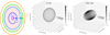 |
Fig. 2 Left panel: Schematic defining the different ellipsoidal shells to model a PN with Co3RaL. The light red area (up to R2) shows the filled shells of the PN. Center and right panels: 3D models of IC 418 and NGC 7027 (see text on Section 3.2 for further details). |
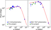 |
Fig. 3 SED of IC 418 (left panel) and NGC 7027 (right panel). Continuous red lines represent the Co3RaL predictions; diamonds display the observational measurements and corresponding errors. The IC 418 data has been taken from Vollmer et al. (2010); Condon et al. (1998); Griffith et al. (1994); Murphy et al. (2010); Wright et al. (2009); Massardi et al. (2009); Bennett et al. (2003); Gold et al. (2011); Chen & Wright (2009), while the NGC 7027 data has been taken from Frew et al. (2016); Condon et al. (1998); Vollmer et al. (2010); Gordon et al. (2021); Becker et al. (1991); Gregory & Condon (1991); Reich et al. (2014); Vollmer et al. (2008); Kellermann & Pauliny-Toth (1973); Sanchez Contreras et al. (1998). |
Summary of the RRL detections (D) and tentative detections (T) by element, source, and mm band.
4 Results for IC 418
The C-rich PN IC 418 has been studied all along the electromagnetic spectrum. The central star is surrounded by an elliptical main nebula, which is enclosed by several low surface brightness structures (shells, rings) and two detached halos (see e.g., Guzmán et al. 2009; Ramos-Larios et al. 2012, and references therein). The IC 418 IR spectrum displays both aliphatic and aromatic molecular bands (see Otsuka et al. 2014), unidentified infrared features (UIRs) (see e.g., Forrest et al. 1981; Hony et al. 2002) and C60 emission bands (Otsuka et al. 2014). However, all previous attempts to detect any molecular emission at radio frequencies have failed so far (see e.g., Dayal & Bieging 1996, where they tried to detect the J = 1–0 and J = 2–1 lines of 12CO after reaching an rms noise of 5 mK in Tmb).
Previous RRL works on this source have reported the detection of H and He I radio spectral lines with Δn = 1–1: H38α, Η39α, Η76α, Η85α, Η91α, H92α, H110α, H95β, H114β, H115β, H16β, Η132γ, Η145δ, and He I 76α, He I 91α, He I 92α, He I 114β, He I 115β, He I 116β, and, He I 132γ (Terzian & Balick 1972; Walmsley et al. 1981; Garay et al. 1989; Dayal & Bieging 1996; Guzman-Ramirez et al. 2016). With the exception of the Η38α and Η39α lines, all previous observations have been made at frequencies < 15 GHz. Therefore, the mm range has thus remained largely unexplored. In Table 3 (and Table B.1) as well as in Figs. 4, 5, we report for the first time detection of 158 previously undetected Η and He I RRLs at 2, 3, and 7 mm in the PN IC 418 as well as the tentative detection of 25 RRLs of the same atoms (the H38α and H39α lines were previously detected, but we do not cover that range). We give examples of the individual line profiles in Appendix A. In Table B.1, we report the upper limits for those Η and He I lines that were not detected.
The results (in terms of peak fluxes and FWHM values) from the radiative transfer model Co3RaL are compatible with the observations within the observational standard deviation. The average FWHM is 28 ± 5 km s–1 for H lines and 16 ± 7 km s–1 for He I lines. The global results of both the observations and the Co3RaL models are summarized in Fig. 6.
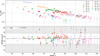 |
Fig. 4 Peak intensity (in Tmb [Κ] units, top panel) and FWHM (in km s–1, bottom panel) of the observed H lines in IC 418. Diamonds represent the 2 mm data, stars the 3 mm data, and dots the 7 mm data. |
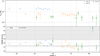 |
Fig. 5 Peak intensity (in Tmb [Κ] units, top panel) and FWHM (in km s–1 in the bottom panel) of the observed He I lines in IC 418. Diamonds represent the 2 mm data, stars the 3 mm data, and dots the 7 mm data. |
4.1 Neutral hydrogen (H) RRLs
The number of detected lines is quite large, so we first compared the lower level involved in the transition, n, with the peak flux and FWHM of each line (see Fig. 4).
We detect lines for Δn ⩽ 13 at 2 and 3 mm. All lines with the same Δn have similar intensities and the intensities decrease as Δn increases. At 7 mm, we can only reach Δn = 10, but we find a strong dispersion of the peak intensities for sets of lines with Δn ⩾ 6. We tentatively detect lines with Δn = 10–13 at 2 mm, Δn = 10–11 at 3 mm, and Δn = 7–10 at 7 mm (see Table B.l for more detailed information).
The FWHM values also show a great dispersion as n grows up (see Fig. 4). We have considered the 1σ standard deviation of the mean value to differentiate between too narrow and broad lines. At 2 mm we find two outliers that display a higher FWHM. These two lines are merged in the spectrum with each other, which makes difficult to find a good Gaussian fit for both. The detections at 3 mm have FWHM values quite close to the mean, except for two cases. The broader line is a line contaminated by an unidentified emission (UF), while the narrower one is a line with a very sharp profile and no contamination. At 7 mm, a large dispersion of the FWHM values starts around n = 90 for Δn ⩾ 7, which are, by far, the weakest lines in this spectral range.
By comparing the observational peak flux values with the modeling, we observe a really good agreement (see Fig. 6 upper panel) within the error bars (that is, a maximum flux calibration uncertainty of 10% combined the Gaussian fit error); even for the weakest lines at 2, 3, and 7 mm.
The FWHM values predicted by the Co3RaL model are very homogeneous. Considering the standard deviation of the observational data, Co3RaL shows a good agreement with the detections at 2 and 3 mm (see Fig. 6 upper panel). At 7 mm, our observations show more dispersion for high Δn values, while the FWHM model values tend to increase with Δn (see also Fig. 7). However, the model is still compatible with the observations.
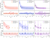 |
Fig. 6 Compatibility of the Co3RaL model data (peak fluxes and FWHM in mJy and km s–1, respectively) with the observational ones for H (upper panel) and He I (lower panel) in PN IC 418. The dots represent the peak flux and FWHM of each observed emission line obtained with the Gaussian fit using the available procedure in CLASS with the respective errors, while the crosses represent the peak flux and FWHM values simulated by Co3RaL. All data are separated by frequency bands. The colored regions on the peak flux plots represent the ±1 σ deviation of the data at each frequency band. The colored regions on the FWHM plots represent the ±1 σ deviation from the observational FWHM mean (see Section 2 for more details). |
4.2 Neutral helium (He I) RRLs
The Fig. 5 shows the observed He I lines in the IC 418 radio spectra. The number of lines is significantly lower than for Η (see also Table 3 and Table B.1) because the intensity of the lines depends on their atomic number and mass, but also because the He I abundance is 10 times lower than Η abundance.
At 2 mm we clearly detect three He I lines. All of them show FWHMs close to the mean value (see bottom panel of Fig. 5).We did not expect to observe more lines in this range, considering the list of frequencies we previously calculated for He I using Eq. (2) and the rms level of our 2mm IC 418 observations.
At 3 mm, there are three detections and one tentative detection. The detected lines display FWHMs very close to the mean with the exception of the broad He I 60γ line. However, this line is blended with H87κ and, as we mentioned above, the parameters of the fit are affected by high uncertainties.
At 7 mm the dispersion of the peak intensities is larger for lines with Δn = 3, which correspond to the weakest He I lines. We only detect half of the He I nγ lines in this frequency range. The FWHMs do not strongly deviate from the mean value.
The agreement of the observational intensity values with the Co3RaL predictions is also very good (see Fig. 6, lower panel). The predicted peak fluxes are statistically compatible with our line detections. The Co3RaL FWHMs are roughly similar to the observed ones. The larger discrepancies appear again at 7 mm (see Section 6 for a more detailed explanation).
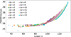 |
Fig. 7 FWHM values (in km s–1 ) from Co3RaL modeling of the RRLs in IC 418 as a function of the lower quantum number, n. Note: the step increases in line width for η larger than 100. Such broadening is not seen or detected in the observations (see Section 6 for more detailed explanations). |
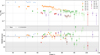 |
Fig. 8 Peak intensity (in Tmb [K ] units, top panel) and FWHM (in km s–1, bottom panel) of the observed H lines in NGC 7027. Diamonds represent the 2 mm data, stars the 3 mm data, and dots the 7 mm data. |
5 Results for NGC 7027
The bipolar and multipolar C-rich PN NGC 7027 is an intriguing and extensively studied source. Many molecules have been detected in this complex PN (see e.g. Zhang et al. 2008), which is thought to host a central binary system (Moraga Baez et al. 2023). The existence of such a binary central star has contributed to its complex morphology. Three main axes or outflows have been confirmed with optical observations, each corresponding to a different ejection jet from the central system. The X-ray emission aligns with the youngest outflow (Montez & Kastner 2018; Moraga Baez et al. 2023) and also enhances the formation of molecules such as HCO+ (Bublitz et al. 2023). Even though the central star has a high effective temperature (Teff = 200 000 K), the rich molecular content seems to be protected by a dusty equatorial belt confirmed by, for instance, Nakashima et al. (2010); Moraga Baez et al. (2023).
The PN NGC 7027 has also been observed in the IR range. Previous studies, such as Beintema et al. (1996), confirm the presence of both aliphatic and aromatic species together with additional UIR features (see e.g. Kwok & Zhang 2011). However, the four strongest IR emission bands of C60 fullerenes are not detected in its ISO/SWS IR spectrum, being classified as a non-C60 PN (Otsuka et al. 2014).
Over the last 60 years, NGC 7027 has been extensively observed at sub-mm frequencies, resulting in the detection of several H RRLs; for example, Η113α, Η85α, H66α, or H107β (see Rubin & Palmer 1971; Terzian & Balick 1972; Chaisson & Malkan 1976; Churchwell et al. 1976; Terzian 1978; Walmsley et al. 1981; Ershov & Berulis 1989; Roelfsema et al. 1991). Additionally, a couple of He I and He II lines have been reported: He I 76α, He II 105α, and He II 121α (Chaisson & Malkan 1976; Terzian 1980; Mezger 1980; Walmsley et al. 1981). The first mm detections were made by Vallee et al. (1990), who observed the source with the IRAM 30m at 99 and 232 GHz, reporting the detection of H30α, He I 30α, H40α, and He I 40α. The most recent and extended survey of NGC 7027 was conducted by Zhang et al. (2008), who reported nine Hnα, nine Hnβ, eight Hnγ, and eight Hel nα lines. Their work was a significant step toward larger and high-sensitivity surveys, highlighting the importance of these kinds of deep radio line surveys for both molecular and RRL detections.
In Table 3 and Figs. 8, 9, and 10, we report the detections and tentative detections of, respectively, 134 and 28 RRLs of H, He I, and He II RRLs (see some examples of individual lines in Appendix A and see Table B.1 for more details). All H lines with Δn ⩾ 4, He I lines for Δn ⩾ 2, as well as all He II, are new detections toward PN NGC 7027.
The radio spectra of this PN are populated by both RRLs and molecular emission lines. Indeed, in some cases, the molecular lines are blended with the RRLs. The peak temperature and the FWHM of the detected lines as well as the comparison between the observational measurements and the Co3RaL model predictions are displayed in Figs. 8, 9, 10, and 11. The average FWHMs for the H, He I, and He II lines are 38 ± 10 km s–1, 29 ± 7 km s–1, and 33 ± 6 km s–1, respectively. Similarly to PN IC 418 (see Fig. 7), the FWHM values predicted by the Co3RaL NGC 7027 model slightly increase, for a fixed Δn, with decreasing frequency.
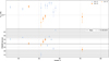 |
Fig. 9 Peak intensity (in Tmb [K] units, top panel) and FWHM (in km s–1, bottom panel) of the observed He I lines in NGC 7027. Diamonds represent the 2 mm data, stars the 3 mm data, and dots the 7 mm data. |
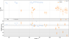 |
Fig. 10 Peak intensity (in Tmb [Κ] units, top panel) and FWHM (in km s–1, bottom panel) of the observed He II lines in NGC 7027. Diamonds represent the 2 mm data, stars the 3 mm data, and dots the 7 mm data. |
5.1 Neutral hydrogen (H) RRLs
The number of Η RRLs detected in NGC 7027 is smaller than for IC 418 (see Table 3 and Table B.l). All this information is plotted in Fig. 8.
The intensities of all the detected lines at 2 mm decrease as the quantum number n grows up. The FWHMs of almost all the lines are close to the mean value. The only exception in this mm band displaying large peak flux error bars and a significantly large FWHM is Η69θ, a line that might be contaminated with extra molecular emission that affects its Gaussian fit.
At 3 mm, we detect all the expected lines with the exception of one line, which is below the detection limit. The high SNR of the Η lines in this band results in high-quality line profile fits. The Η RRLs with the same Δn value show similar peak fluxes within the error bars. The FWHMs are statistically compatible between the different observational bands; except for the H86κ line. The latter line clearly deviates from the average, displaying a FWHM ~65 km s–1. Such broadening is probably due to strong blending with an unidentified molecular line that modifies the RRL shape.
At 7 mm, we find again more variability, specially for Δn ⩾ 5. The higher rms level at sub-bands 5–8 (these correspond to ~42–50 GHz and it is produced by resonant signals in the receiver) hides several high-Δn H lines that we clearly detect at the lower frequency sub-bands. In general, clear detections deviate less significantly from the mean than the tentatives ones, but there are exceptions along the full frequency range.
The Co3RaL model predicts peak intensities similar to those observed (see Fig. 11 upper panel). The synthetic FWHM s match up quite well with the observational results at 2 and 3 mm. Once more, the model predictions at 7 mm show an increasing FWHM value with Δn that it is not evident in the observations. This effect is the same that we observed above in the Co3RaL model results for IC 418 (see Fig. 7).
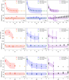 |
Fig. 11 Compatibility of Co3RaL model data (peak fluxes and FWHM in mJy and km s–1, respectively) with the observational ones for H (upper panel), He I (middle panel), and He II (lower panel) in PN NGC 7027. Color and label codes are the same as in Fig. 6. |
5.2 Neutral helium (He I) RRLs
The 2 mm band is the only one in which we detect He I lines for Δn ⩽ 3. At 3 and 7 mm, we only observe lines with Δn ⩽ 2 (see Fig. 9). In the 2 mm range, the stronger lines are blended with other H or He II RRLs and their line profiles were difficult to fit. However, their FWHM values do not deviate much from the mean and remain inside the 1σ region in Fig. 9. At 3 mm, the three detected lines are blended with He II lines. Only one of them has a FWHM value clearly outside the region delimited by the standard deviation, suggestive of the blending just mentioned before. At 7 mm, we only have detected clear He I nα lines, but only one He I nβ line due to an insufficient sensitivity. This fact naturally implies a larger dispersion from the mean standard deviation value for most of the 7 mm He I detections.
Finally, the Co3RaL predictions are compatible with the peak intensities of all detected He I lines, even the weaker ones (see Fig. 11 middle panel). The predicted FWHMs are also statistically compatible with the observations.
5.3 Ionized helium (He II) RRLs
The strong UV and X-ray emission in NGC 7027 allows for the presence of He II lines, which are a bit stronger than the He I ones. At 2 and 3 mm, we only find clear detections of He II lines with Δn ⩽ 3. They display FWHM values very close to the mean, except for He II 84β. This individual line has a FWHM close to 50 km s–1, but it is strongly blended with He I 42α, which is slightly stronger and affects the line fit.
At 7 mm, we detect all He II nα lines in the frequency range and most of the He II nβ lines. They display similar peak intensities with larger error bars toward the upper end of the band range. The FWHM values of the He II nα lines do not strongly deviate from the mean. The only exception is He II 87α, partially blended with H78γ. The He II nβ lines are weaker, so their FWHMs display larger deviations from the mean value. At the upper end of the 7 mm range (~42.5 GHz), we cannot find clear detections because all lines lie below the 3σ detection limit. The dispersion around the mean is larger than at 2 and 3 mm, probably caused by the intrinsic weakness of the lines.
For He II, the Co3RaL modeling reproduces quite well the observational peak fluxes at 3 and 7 mm, but at 2 mm the predicted peak fluxes are higher than the observed ones (see Fig. 11 lower panel). The FWHMs are in good agreement for all frequency ranges, right in the standard deviation limit. At 7 mm, the progressive broadening of the Co3RaL synthetic lines is observed, as in the previous cases.
6 Discussion and applications to radio spectroscopy
The different number of detections on each source for each element (see Table 3 and Table B.1) is mainly due to the higher sensitivity, but it may also be a direct consequence of the effective temperature of their respective central star and/or their intrinsic brightness. The central star (CS) of IC 418 has a lower effective temperature (~30 000 K), so it provides less energetic photons to its surrounding nebula. Even though we have detected a higher number of H RRLs than in NGC 7027, there is no sign of He II RRLs in IC418. This finding is completely logical: a higher effective temperature of the NGC 7027 CS generates a stronger UV radiation, providing enough energetic photons to ionize He I to He II and He III. The nebular age for each PN is also important. NGC 7027 is significantly younger than IC 418, with its hotter CS producing more energetic UV radiation and the previously expelled circumstellar material being closer to the CS.
We did not observe any RRLs of a species heavier than He. The ionization potential of C I recombination lines (11.26 eV) is lower than that of H (13.6 eV), so in the case of ionization-bounded PNe, only the photons with energies in the range 11.26-13.6 eV can escape and photoionize C atoms outside the H II region. C I RRLs would be expected to be wide spread throughout the PN because C is ejected from the CS simultaneously than H and He. However, the C abundance (3 · 10–4–7 · 10–4; Pottasch et al. 2004) is relatively low compared to H and He (which display abundances of 0.9 and 0.09, respectively; Pottasch et al. 2004). With this abundance, detecting C I RRLs requires data with significantly lower noise levels (the modeling predicts intensities of ~10–3 mK) or a meaningful opacity enhancement related, for instance, to high density shells. Indeed, the C I lines have been detected coming from outside the H II regions of NGC 7009 (Akras et al. 2024) showing a bipolar structure, which is likely associated with the interaction of low expanding neutral shells and more recent higher velocity outflows. Our beam is probably smaller than the neutral shells outside the H II region of NGC 7027 and the high velocity winds known to exist in this PN expand in a different direction to the line-of-sight. The emission related to possible interactions like those in NGC 7009 are likely absent in our NGC 7027 data but mapping this PN in a wider field-of-view could unveil C I RRLs emission.
Interestingly, the observed He lines are narrower than the H ones for both sources. In the case of IC 418, the range of FWHMs slightly overlaps (28 ± 5 km s–1 and 16 ± 7 km s–1 for H and He I, respectively), but the FWHM distributions for H and He can be taken as statistically different. This clear difference may indicate that the emission from the atomic H and He lines comes from specific locations across the nebula. The first ionization energy for He is 24.6 eV (Kandula et al. 2011); namely, almost twice as high as the H ionization energy, while the second ionization energy for He is 54.4 eV (Yerokhin & Shabaev 2015). This means that only the most energetic photons can ionize the He atoms and these energetic photons should be mostly absorbed closer to the CS. This is because the opacity of the gas increases for shorter wavelengths. As we move away from the CS, there are less photons energetic enough to ionize other species than H atoms. The majority of the emission of ionized He producing RRLs is located close to the CS because the energetic photons are absorbed there. Therefore, H RRLs mostly trace the outer shells of the ionized nebula, while He RRLs trace the inner parts (with a smaller solid angle than the outer layers). Moreover, having different layers traced by different species relates the distinct FWHMs with a radial velocity gradient.
The broadening of RRLs is the convolution of two main components: the Gaussian contribution and the gas expansion velocity effects (see e.g., Kielkopf 1973; Báez-Rubio et al. 2013). The Gaussian contribution is produced by thermal and turbulent motions. For the IC 418 H RRLs, this gives FWHM ~10 km s–1; in other words, H RRLs narrower than observed and predicted, with FWHM ~28 ± 5 km s–1. Thus, the total broadening of RRLs is mainly dominated by the expansion velocity. Therefore, wider lines come from outer shells than narrower ones. In the specific case of IC 418, the gas closer to the CS (traced by He I) expands slower than the gas from the outer layers (traced by H).
The situation for NGC 7027 is apparently more complicated. The three FWHM mean values are 38 ± 10 km s–1, 29 ± 7 km s–1, and 33 ± 6 km s–1 for H, He I, and He II lines, respectively, so the ranges overlap. In contrast with IC 418, in which given a FWHM value of any line we can determine without doubts if it is a H or a He I RRL, in NGC 7027 the lines are statistically similar. Consequently, most of the expected gas acceleration occurs within the region where He is ionized and beyond the gas can be assumed to expand at velocities close to the terminal value. One of the main differences between both PNe is that the CS of NGC 7027 has an effective temperature of ~200 000 K (while Teff ~ 30 000 K for IC 418 CS), so there are more energetic photons. As they move away from the CS, they interact with the gas around the star ionizing it and losing energy. However, the photons emitted through the recombination processes are still energetic enough at larger distances than for IC 418. Therefore, He can be ionized and recombined at further distances and there is not a clearly differentiated region where one species dominates over the other.
The good agreement between the Co3RaL results and the detected lines demonstrates the good quality of the models when modeling and predicting an unprecedented amount ofRRLs. The Co3RaL predictions point out that the tentative lines in the spectra are indeed below the detection level, which means that these lines are very likely real and could be finally confirmed if we performed yet deeper integrations. The model reproduces quite well the FWHM values of the H and He lines for both sources. We remark that only Te values of 22 000–25 000 K can reproduce simultaneously both the SED and all RRLs of H and He in NGC 7027. The Te values derived from other lines such as [O III] did not reproduce the SED and/or all RRLs. See, for example, the work by Zhang et al. (2005) and their temperature estimates based on collisionally excited lines and optical recombination lines in this source. Their results using collisionally excited lines show values of 10 400 K ([O I] λ5577/(λ6300 + λ6363)) or 8100K ([C I] (λ9824 + λ9850)/λ8727), which also differ from the results of the Balmer jump temperature obtained using otherlines in the optical range radiatively excited (12 600K from the [O III] (λ4959 + λ5007)/λ4363 or 18 700 K from the [O II] (λ7320 + λ7330)/λ3726). These kinds of discrepancies were noticed long ago, along with the fact that collisionally excited temperatures are lower than those derived from continuum measurements see e.g., Miller & Mathews 1972). Recently, authors as Sánchez Contreras et al. (2024) have also warned about the impossibility of deriving Te values from the collisionally excited lines reproducing the SED of the pre-PN M2-9 at mm frequencies. The discrepancy between Te derived from the RRL and from collisionally excited lines as [O III] is still an open question. Nevertheless, Krabbe & Copetti (2005) showed a strong dependence of Te with ne, which suggests that ne and associated spatial structures could be playing a relevant role. Therefore, further research is needed to solve these discrepancies and provide a robust explanation.
Furthermore, no maser amplification is expected according to our models. After obtaining the set of model parameters that best fit both the RRLs and the SED, we looked for the combination of Te and ne producing maser emission in IC 418. Independently of Te, the maser amplification effect is predicted for ne > 3 · 104 cm–3, which is higher than our best estimate. We have to point out that maser amplification also requires optical paths along the line of sight producing enough coherence in velocity to allow for an exponential amplification. In our models, most of the emission is produced in a relatively thin shell and there is no combination of Te and ne that would produce a maser amplification. Therefore, considering both the required conditions for maser amplification and model results, we can confidently rule out any maser emission in IC 418. Similar results and conclusions were obtained for NGC 7027.
The predicted FWHMs display an interesting behavior as frequency decreases or as nlower increase (see Fig. 7). The RRLs seem to be wider, but we do not observe this tendency in the observational results. This broadening is a feature of the model. The intensity of the lines depends directly on their Einstein coefficients, which are calculated using the Gaunt factors. Considering LTE or non-LTE provides slightly different results for the Gaunt factors. The Co3RaL code uses the non-LTE Gaunt factors only for nlower ≤ 100. Lines with nlower ≥ 100 (observed in the 7 mm range) use the LTE Gaunt factors to calculate their Einstein coefficients. Even though the difference is quite small, the opacity of the lines with the LTE Gaunt factor is slightly larger than that of the lines using non-LTE Gaunt factors. This is, the opacity of lines with nlower ≥ 100 (LTE) is slightly larger than the opacity of lines with nlower ≤ 100 (non-LTE). The final effect of this changing of the thermodynamic regime is a broadening of the lines with nlower ≥ 100, which are only visible at 7 mm. Finding a computationally efficient way to obtain the non-LTE Gaunt factors for nlower ≥ 100 would correct this effect.
The outputs (specifically, physical parameters) of Co3RaL offer useful information about the physical characteristics of both PNe. This information is given in Table 2. The outputs of IC 418 are compatible with the bibliography (see e.g., Morisset & Georgiev 2009; Ramos-Larios et al. 2012). We obtained a mean kinematic timescale compatible with the timescale of Dopita et al. (2017). The mass-loss rate is similar, but higher than that derived by Dopita et al. (2017) using post-AGB evolutionary models. This fact also justifies the different timescales. Our model only reproduces the observed peak intensities of all H, He I RRLs with a Te higher than previous works (see e.g., Pottasch et al. 2004; Morisset & Georgiev 2009; Ramos-Larios et al. 2012; Dopita et al. 2017). In the case of NGC 7027, the physical parameters derived from Co3RaL are also compatible with previous results. The timescales vary from 600–700 a (Masson 1989; Latter et al. 2000), making our kinematic timescale results compatible with previous models (see also Moraga Baez et al. 2023). There has been a wide range of Te, which strongly depend on the spectral line used to calculate them (see e.g., Chaisson & Malkan 1976; Atherton et al. 1979; Walmsley et al. 1981; Bernard Salas et al. 2001). It is interesting to point out that we obtained very similar ionized masses for both PNe as Santander-García et al. (2022), which used quite different data analysis methods.
The RRLs are a very useful tool for studying ionized gas regions, and more precisely, PNe. The measurement of RRLs of different elements is also a fundamental tool to analyze the atomic emission and its role in the evolution of the system. However, the knowledge of their existence could be very useful for molecular radio spectroscopy in ionized regions, where RRLs are present and might be mixed up with molecules.
The unambiguous detection of a molecular species in space is a difficult task. The list of identified individual species (including isotopologues) grows up to ~300 (McGuire 2022). However, there are hundreds of UFs that have not been assigned to any molecular transition yet. The main difficulty is to estimate the spectra of molecules that are commonly hard to be synthesized in the laboratory or which cannot be determined with enough accuracy by means of complex ab initio calculations. The geometry of the molecule, a large number of atoms, or many overlapped electronic states increase the complexity of this task. Therefore, the largest molecules identified in space through their rotational transitions up to date have no more than 25 atoms (see Cernicharo et al. 2024b).
The number of possible molecular carriers that might be associated with UFs is thus very large. The limitation of the number of truly UFs is crucial and this is usually done in two ways: (i) by comparing the UF frequencies with (public or private) molecular databases and (ii) identifying atomic emission lines. The RRL catalogs presented here may play a key role on this problem of the identification of the UF carriers. The identification of RRLs in our sample of sources allowed us to correctly associate the atomic emission lines with their atomic carriers (specifically, H and He) and list the remaining emission lines (namely, UFs) to be associated with their still unknown molecular carriers. By ignoring the RRLs in IC 418, a peculiar PN without any known molecule detected at radio wavelengths, would have led us to deal with dozens of emission lines (UFs) that do not correspond to molecular transition frequencies. In the case of NGC 7027, a PN with confirmed molecular emission at mm wavelengths, we could correctly identify some RRLs emission contamination to well known molecular emission lines as well as some molecular emission contamination to the RRLs. In short, the detection of the most intense RRLs of H and He made possible to correctly model both sources and predict the peak intensities of much weaker lines, as well as to distinguish their atomic or molecular origin.
7 Conclusions
The unprecedented high-sensitivity mm data obtained toward PNe IC 418 and NGC 7027 at three frequency bands have enabled us to report, for the first time, the detection of 323 RRLs. Many of them had never detected before in a PN or even in any astrophysical source. Additionally, other 50 weak features along the three frequency bands and below the 3σ detection limit could be tentatively identified as RRLs. Every emission line was carefully compared with a complete list of RRL frequencies of H, He I, and He II. Those emission lines coincident with the frequency of a RRL have been carefully fitted with a Gaussian function and modeled with the Co3RaL radiative transfer model. The spectra derived from Co3RaL are compatible with the observational results within the error bars across the frequency ranges observed with the IRAM 30m and RT40m radio telescopes. We also obtained the main nebular physical parameters from Co3RaL to describe the physical characteristics of the sources.
These catalogs of detected H, He I, and He II RRLs toward two C-rich PNe constitute a significant breakthrough for a better understanding and characterization of the chemical environment of a PN. The reported lines confirm the presence of many RRLs that had not been observed or identified in previous studies. A revision on ionized sources should be done to be sure if some UFs are RRLs or some molecular emission lines are contaminated by RRLs.
The detection of this large number of RRLs leaves some open questions that have to be confirmed with interferometric maps and lower frequency observations. First, we consider whether the spatial distribution of the species is similar to what was derived from the modeling and whether RRLs of heavier elements would be detectable toward denser regions of the PNe. Furthermore, if RRLs become broader at lower frequencies, there could be a limit on differentiating them with ripples in the spectra, while RRLs at lower frequencies might provide different (or more) information on the sources. It would be interesting to have a better knowledge on the behavior of RRLs at lower frequencies and to check whether a limit on the detections exists.
The study and characterization of RRLs seems to be regaining importance in the field. New developments in receivers and radio telescopes provide the proper tools to perform this kind of sensitive and high-precision analysis of astronomical sources, which are essential to correctly confirm atomic and molecular emission lines in space. A better understanding of RRLs will improve our knowledge of the physics and chemistry of the emitting regions. The RRL catalogs presented here provide a tool to identify radio emission lines and to know which ones are truly produced by molecules. This can aid in the identification of new molecular species, improving our present understanding of the molecular formation pathways in space. In particular, the results presented in this paper have provided us with lists of weak molecular UFs toward both PNe (in other words, still unidentified emission lines that are not RRLs). Our next efforts will focus on the identification of the molecular carriers producing such weak and unidentified radio emission lines in PNe.
Data availability
Additional Figures A.1–A.29 can be found in Appendix A. Table B.1 is available at the CDS via https://cdsarc.cds.unistra.fr/viz-bin/cat/J/A+A/700/A194
Acknowledgements
The authors acknowledge Miguel Santander-García from the OAN for carrying out the observations at the Yebes RT40m. THR, DAGH, AMT, and RB acknowledge the support from the State Research Agency (AEI) of the Ministry of Science, Innovation and Universities (MICIU) of the Government of Spain, and the European Regional Development Fund (ERDF), under grants PID2020-115758GB-I00/AEI/10.13039/501100011033 and PID2023-147325NB-I00/AEI/10.13039/501100011033. THR acknowledges support from grant PID2020-115758GB-I00/PRE2021-100042 financed by MCIN/AEI/10.13039/501100011033 and the European Social Fund Plus (ESF+). JA, JPF, JJDL, and VB are partially supported by I+D+i projects PID2019-105203GB-C21 and PID2023-146056NB-C21, funded by the Spanish MCIN/AEI/10.13039/501100011033 and EU/ERDF. JPF also acknowledges support from grants PID2023-147545NB-I00 and PID2023-146056NB-C22. MAGM acknowledge to be funded by the European Union (ERC, CET-3PO, 101042610). Views and opinions expressed are however those of the author(s) only and do not necessarily reflect those of the European Union or the European Research Council Executive Agency. Neither the European Union nor the granting authority can be held responsible for them. This work is based on observations carried out under project number 158-21 with the IRAM 30m telescope. IRAM is supported by INSU/CNRS (France), MPG (Germany) and IGN (Spain). Based on observations carried out with the Yebes 40 m telescope (22A011). The 40 m radio telescope at Yebes Observatory is operated by the Spanish Geographic Institute (IGN; Ministerio de Transportes y Movilidad Sostenible). This publication is based upon work from COST Action CA21126 – Carbon molecular nanostructures in space (NanoSpace), supported by COST (European Cooperation in Science and Technology).
References
- Agúndez, M., Cernicharo, J., & Guélin, M. 2014, A&A, 570, A45 [Google Scholar]
- Akras, S., Monteiro, H., Walsh, J. R., et al. 2024, A&A, 689, A14 [NASA ADS] [CrossRef] [EDP Sciences] [Google Scholar]
- Ali, A., Ismail, H. A., & Alsolami, Z. 2015, Ap&SS, 357, 21 [Google Scholar]
- Atherton, P. D., Hicks, T. R., Reay, N. K., et al. 1979, ApJ, 232, 786 [Google Scholar]
- Báez Rubio, A. 2015, PhD thesis, Complutense University of Madrid, Spain [Google Scholar]
- Becker, R. H., White, R. L., & Edwards, A. L. 1991, ApJS, 75, 1 [Google Scholar]
- Beintema, D. A., van den Ancker, M. E., Molster, F. J., et al. 1996, A&A, 315, L369 [Google Scholar]
- Bennett, C. L., Hill, R. S., Hinshaw, G., et al. 2003, ApJS, 148, 97 [Google Scholar]
- Bernard Salas, J., Pottasch, S. R., Beintema, D. A., & Wesselius, P. R. 2001, A&A, 367, 949 [NASA ADS] [CrossRef] [EDP Sciences] [Google Scholar]
- Bignell, R. C. 1974, ApJ, 193, 687 [Google Scholar]
- Brocklehurst, M. 1970, MNRAS, 148, 417 [NASA ADS] [CrossRef] [Google Scholar]
- Brocklehurst, M. 1971, MNRAS, 153, 471 [Google Scholar]
- Bublitz, J., Kastner, J. H., Santander-García, M., et al. 2019, A&A, 625, A101 [NASA ADS] [CrossRef] [EDP Sciences] [Google Scholar]
- Bublitz, J., Kastner, J. H., Hily-Blant, P., et al. 2023, ApJ, 942, 14 [Google Scholar]
- Báez-Rubio, A., Martín-Pintado, J., Thum, C., & Planesas, P. 2013, A&A, 553, 16 [Google Scholar]
- Cabezas, C., Pardo, J. R., Agúndez, M., et al. 2023, A&A, 672, L12 [NASA ADS] [CrossRef] [EDP Sciences] [Google Scholar]
- Cami, J., Bernard-Salas, J., Peeters, E., & Malek, S. E. 2010, Science, 329, 1180 [NASA ADS] [CrossRef] [Google Scholar]
- Carter, M., Lazareff, B., Maier, D., et al. 2012, A&A, 538, A89 [NASA ADS] [CrossRef] [EDP Sciences] [Google Scholar]
- Cernicharo, J., Agúndez, M., Velilla Prieto, L., et al. 2017, A&A, 606, L5 [NASA ADS] [CrossRef] [EDP Sciences] [Google Scholar]
- Cernicharo, J., Cabezas, C., Pardo, J. R., et al. 2019, A&A, 630, L2 [NASA ADS] [CrossRef] [EDP Sciences] [Google Scholar]
- Cernicharo, J., Cabezas, C., Pardo, J. R., et al. 2023, A&A, 672, L13 [NASA ADS] [CrossRef] [EDP Sciences] [Google Scholar]
- Cernicharo, J., Cabezas, C., Agúndez, M., et al. 2024a, A&A, 686, L15 [NASA ADS] [CrossRef] [EDP Sciences] [Google Scholar]
- Cernicharo, J., Cabezas, C., Fuentetaja, R., et al. 2024b, A&A, 690, L13 [NASA ADS] [CrossRef] [EDP Sciences] [Google Scholar]
- Chaisson, E. J., & Malkan, M. A. 1976, ApJ, 210, 108 [NASA ADS] [CrossRef] [Google Scholar]
- Chen, X., & Wright, E. L. 2009, ApJ, 694, 222 [Google Scholar]
- Churchwell, E., Terzian, Y., & Walmsley, M. 1976, A&A, 48, 331 [NASA ADS] [Google Scholar]
- Condon, J. J., Cotton, W. D., Greisen, E. W., et al. 1998, AJ, 115, 1693 [Google Scholar]
- Dayal, A., & Bieging, J. H. 1996, ApJ, 472, 703 [Google Scholar]
- Dieter, N. H. 1967, ApJ, 150, 435 [Google Scholar]
- Dopita, M. A., Ali, A., Sutherland, R. S., Nicholls, D. C., & Amer, M. A. 2017, MNRAS, 470, 839 [NASA ADS] [CrossRef] [Google Scholar]
- Ershov, A. A., & Berulis, I. I. 1989, Sov. Astron. Lett., 15, 178 [Google Scholar]
- Forrest, W. J., Houck, J. R., & McCarthy, J. F. 1981, ApJ, 248, 195 [Google Scholar]
- Frew, D. J., Parker, Q. A., & Bojicic, I. S. 2016, MNRAS, 455, 1459 [Google Scholar]
- Garay, G., Gathier, R., & Rodriguez, L. F. 1989, A&A, 215, 101 [Google Scholar]
- García-Lario, P. 2006, in IAU Symposium, 234, Planetary Nebulae in our Galaxy and Beyond, eds. M. J. Barlow, & R. H. Méndez, 63–70 [Google Scholar]
- García-Hernádez, D. A., Manchado, A., Garcia-Lario, P., et al. 2010, ApJ, 724, L39 [CrossRef] [Google Scholar]
- Gold, B., Odegard, N., Weiland, J. L., et al. 2011, ApJS, 192, 15 [Google Scholar]
- Goldberg, L. 1970, Astrophys. Lett., 5, 151 [Google Scholar]
- Gόmez-Muñoz, M. A., García-Hernández, D. A., Barzaga, R., Manchado, A., & Huertas-Roldán, T. 2024, A&A, 682, L18 [Google Scholar]
- González-Santamaría, I., Manteiga, M., Manchado, A., et al. 2021, A&A, 656, A51 [NASA ADS] [CrossRef] [EDP Sciences] [Google Scholar]
- Gordon, Y. A., Boyce, M. M., O’Dea, C. P., et al. 2021, ApJS, 255, 30 [NASA ADS] [CrossRef] [Google Scholar]
- Gregory, P. C., & Condon, J. J. 1991, ApJS, 75, 1011 [Google Scholar]
- Griffith, M. R., Wright, A. E., Burke, B. F., & Ekers, R. D. 1994, ApJS, 90, 179 [NASA ADS] [CrossRef] [Google Scholar]
- Gupta, H., Changala, P. B., Cernicharo, J., et al. 2024, ApJ, 966, L28 [Google Scholar]
- Guzmán, L., Loinard, L., G?mez, Y., & Morisset, C. 2009, AJ, 138, 46 [Google Scholar]
- Guzman-Ramirez, L., Rizzo, J. R., Zijlstra, A. A., et al. 2016, MNRAS, 460, L35 [Google Scholar]
- Herwig, F. 2005, ARA&A, 43, 435 [NASA ADS] [CrossRef] [Google Scholar]
- Hony, S., Waters, L. B. F. M., & Tielens, A. G. G. M. 2002, A&A, 390, 533 [NASA ADS] [CrossRef] [EDP Sciences] [Google Scholar]
- Hummer, D. G., & Storey, P. J. 1987, MNRAS, 224, 801 [NASA ADS] [CrossRef] [Google Scholar]
- Hummer, D. G., & Storey, P. J. 1992, MNRAS, 254, 277 [NASA ADS] [Google Scholar]
- Kandula, D. Z., Gohle, C., Pinkert, T. J., Ubachs, W., & Eikema, K. S. E. 2011, Phys. Rev. A, 84, 062512 [Google Scholar]
- Karakas, A. I., & Lattanzio, J. C. 2014, PASA, 31, e030 [NASA ADS] [CrossRef] [Google Scholar]
- Kardashev, N. S. 1959, Soviet Ast., 3, 813 [Google Scholar]
- Kellermann, K. I., & Pauliny-Toth, I. I. K. 1973, AJ, 78, 828 [NASA ADS] [CrossRef] [Google Scholar]
- Kielkopf, J. F. 1973, J. Opt. Soc. Am., 63, 987 [NASA ADS] [CrossRef] [Google Scholar]
- Krabbe, A. C., & Copetti, M. V. F. 2005, A&A, 443, 981 [NASA ADS] [CrossRef] [EDP Sciences] [Google Scholar]
- Kwok, S. 2016, A&A Rev., 24, 8 [Google Scholar]
- Kwok, S., & Zhang, Y. 2011, Nature, 479, 80 [NASA ADS] [CrossRef] [Google Scholar]
- Latter, W. B., Dayal, A., Bieging, J. H., et al. 2000, ApJ, 539, 783 [NASA ADS] [CrossRef] [Google Scholar]
- Massardi, M., L?pez-Caniego, M., González-Nuevo, J., et al. 2009, MNRAS, 392, 733 [Google Scholar]
- Masson, C. R. 1989, ApJ, 336, 294 [NASA ADS] [Google Scholar]
- McGuire, B. A. 2022, ApJS, 259, 30 [NASA ADS] [CrossRef] [Google Scholar]
- Mezger, P. G. 1980, in Astrophysics and Space Science Library, 80, Radio Recombination Lines, eds. P. A. Shaver, 81 [NASA ADS] [CrossRef] [Google Scholar]
- Mezger, P. G., & Hoglund, B. 1967, ApJ, 147, 490 [NASA ADS] [CrossRef] [Google Scholar]
- Mezger, P. G., & Palmer, P. 1968, Science, 160, 29 [Google Scholar]
- Miller, J. S., & Mathews, W. G. 1972, ApJ, 172, 593 [NASA ADS] [CrossRef] [Google Scholar]
- Montez, R. J., & Kastner, J. H. 2018, ApJ, 861, 45 [NASA ADS] [CrossRef] [Google Scholar]
- Moraga Baez, P., Kastner, J. H., Balick, B., Montez, R., & Bublitz, J. 2023, ApJ, 942, 15 [NASA ADS] [CrossRef] [Google Scholar]
- Morisset, C., & Georgiev, L. 2009, A&A, 507, 1517 [NASA ADS] [CrossRef] [EDP Sciences] [Google Scholar]
- Murphy, T., Sadler, E. M., Ekers, R. D., et al. 2010, MNRAS, 402, 2403 [Google Scholar]
- Nakashima, J.-i., Kwok, S., Zhang, Y., & Koning, N. 2010, AJ, 140, 490 [Google Scholar]
- Otsuka, M., Kemper, F., Cami, J., Peeters, E., & Bernard-Salas, J. 2014, MNRAS, 437, 2577 [NASA ADS] [CrossRef] [Google Scholar]
- Pardo, J. R., Cabezas, C., Agúndez, M., et al. 2023, A&A, 677, A55 [NASA ADS] [CrossRef] [EDP Sciences] [Google Scholar]
- Pardo, J. R., Cernicharo, J., Tercero, B., et al. 2022, A&A, 658, A39 [NASA ADS] [CrossRef] [EDP Sciences] [Google Scholar]
- Pottasch, S. R., Bernard-Salas, J., Beintema, D. A., & Feibelman, W. A. 2004, A&A, 423, 593 [NASA ADS] [CrossRef] [EDP Sciences] [Google Scholar]
- Ramos-Larios, G., Vázquez, R., Guerrero, M. A., et al. 2012, MNRAS, 423, 3753 [Google Scholar]
- Reich, W., Sun, X. H., Reich, P., et al. 2014, A&A, 561, A55 [NASA ADS] [CrossRef] [EDP Sciences] [Google Scholar]
- Rodríguez, L. F., G?mez, Y., & Guzmán, L. 2009, Rev. Mexicana Astron. Astrofis., 45, 85 [Google Scholar]
- Roelfsema, P. R., Goss, W. M., Pottasch, S. R., & Zijlstra, A. 1991, A&A, 251, 611 [Google Scholar]
- Rubin, R. H., & Palmer, P. 1971, Astrophys. Lett., 8, 79 [Google Scholar]
- Sanchez Contreras, C., Alcolea, J., Bujarrabal, V., & Neri, R. 1998, A&A, 337, 233 [NASA ADS] [Google Scholar]
- Sánchez Contreras, C., Tafoya, D., Fonfría, J. P., et al. 2024, A&A, 692, A151 [NASA ADS] [CrossRef] [EDP Sciences] [Google Scholar]
- Santander-García, M., Jones, D., Alcolea, J., Bujarrabal, V., & Wesson, R. 2022, A&A, 658, A17 [NASA ADS] [CrossRef] [EDP Sciences] [Google Scholar]
- Schmidt, D. R., Gold, K. R., Sinclair, A., Bergstrom, S., & Ziurys, L. M. 2022, ApJ, 927, 46 [Google Scholar]
- Storey, P. J., & Hummer, D. G. 1988, MNRAS, 231, 1139 [NASA ADS] [Google Scholar]
- Storey, P. J., & Hummer, D. G. 1995, MNRAS, 272, 41 [NASA ADS] [CrossRef] [Google Scholar]
- Terzian, Y. 1978, in Planetary Nebulae, 76, ed. Y. Terzian, 111 [Google Scholar]
- Terzian, Y. 1980, in Astrophysics and Space Science Library, 80, Radio Recombination Lines, ed. P. A. Shaver, 75 [NASA ADS] [CrossRef] [Google Scholar]
- Terzian, Y., & Balick, B. 1972, Astrophys. Lett., 10, 41 [Google Scholar]
- Tielens, A. G. G. M. 2005, The Physics and Chemistry of the Interstellar Medium (Cambridge University Press) [Google Scholar]
- Tielens, A. G. G. M., Waters, L. B. F. M., & Bernatowicz, T. J. 2005, in Astronomical Society of the Pacific Conference Series, 341, Chondrites and the Protoplanetary Disk, eds. A. N. Krot, E. R. D. Scott, & B. Reipurth, 605 [Google Scholar]
- Tuo, J., Li, X., Sun, J., et al. 2024, ApJS, 271, 45 [Google Scholar]
- Vallee, J. P., Guilloteau, S., Forveille, T., & Omont, A. 1990, A&A, 230, 457 [NASA ADS] [Google Scholar]
- Vollmer, B., Krichbaum, T. P., Angelakis, E., & Kovalev, Y. Y. 2008, A&A, 489, 49 [NASA ADS] [CrossRef] [EDP Sciences] [Google Scholar]
- Vollmer, B., Gassmann, B., Derrière, S., et al. 2010, A&A, 511, A53 [NASA ADS] [CrossRef] [EDP Sciences] [Google Scholar]
- Walmsley, C. M., Churchwell, E., & Terzian, Y. 1981, A&A, 96, 278 [NASA ADS] [Google Scholar]
- Wright, E. L., Chen, X., Odegard, N., et al. 2009, ApJS, 180, 283 [NASA ADS] [CrossRef] [Google Scholar]
- Yerokhin, V. A., & Shabaev, V. M. 2015, J. Phys. Chem. Ref. Data 44, 033103 [Google Scholar]
- Zhang, Y., Liu, X.-W., Luo, S.-G., Péquignot, D., & Barlow, M. J. 2005, A&A, 442, 249 [NASA ADS] [CrossRef] [EDP Sciences] [Google Scholar]
- Zhang, Y., Kwok, S., & Dinh-V-Trung. 2008, ApJ, 678, 328 [Google Scholar]
The RRLs are emission lines in the radio regime produced when an electron drops from a higher energy level of an atom or ion to a lower energy level.
Greek letters correspond to the following electronic level gaps: α → Δn = 1, β → Δn = 2, γ → Δn = 3, δ → Δn = 4, ϵ → Δn = 5, ζ → Δn = 6, η → Δn = 7, θ → Δn = 8, ι → Δn = 9, κ → Δn = 10, λ → Δn = 11, μ → Δn = 12, ν → Δn = 13.
IRAM is an international research institute. Founded in 1979, it is participated in by the French Centre National de la Recherche Scientifique (CNRS), the German Max-Planck-Gesellschaft (MG), and the Spanish Instituto Geográfico Nacional (IGN) through the Observatorio Astronόmico Nacional (OAN). IRAM operates the single-dish 30m telescope in Spain and the NOEMA interferometer in the French Alps.
GILDAS is a collection of state-of-the-art software oriented toward (sub-)millimeter radio-astronomical applications (either single-dish or interferometric). The GILDAS developments are supported by IPAG (Observatoire de Grenoble) and IRAM, with additional contributions from LAB (Observatoire de Bordeaux) and LERMA (Observatoire de Paris). For more information, see https://www.iram.fr/IRAMFR/GILDAS (accessed on 24 September 2024).
All Tables
Summary of the RRL detections (D) and tentative detections (T) by element, source, and mm band.
All Figures
|
Fig. 1 Examples of the RT40m spectrum of IC 418 (left) and the IRAM 30 m spectrum of NGC 7027 (right). The gray arrow on the right panel indicates an absorption feature produced by some molecule in the line of sight of NGC 7027 (probably from a cold shell of its molecular envelope). |
| In the text | |
|
Fig. 2 Left panel: Schematic defining the different ellipsoidal shells to model a PN with Co3RaL. The light red area (up to R2) shows the filled shells of the PN. Center and right panels: 3D models of IC 418 and NGC 7027 (see text on Section 3.2 for further details). |
| In the text | |
|
Fig. 3 SED of IC 418 (left panel) and NGC 7027 (right panel). Continuous red lines represent the Co3RaL predictions; diamonds display the observational measurements and corresponding errors. The IC 418 data has been taken from Vollmer et al. (2010); Condon et al. (1998); Griffith et al. (1994); Murphy et al. (2010); Wright et al. (2009); Massardi et al. (2009); Bennett et al. (2003); Gold et al. (2011); Chen & Wright (2009), while the NGC 7027 data has been taken from Frew et al. (2016); Condon et al. (1998); Vollmer et al. (2010); Gordon et al. (2021); Becker et al. (1991); Gregory & Condon (1991); Reich et al. (2014); Vollmer et al. (2008); Kellermann & Pauliny-Toth (1973); Sanchez Contreras et al. (1998). |
| In the text | |
|
Fig. 4 Peak intensity (in Tmb [Κ] units, top panel) and FWHM (in km s–1, bottom panel) of the observed H lines in IC 418. Diamonds represent the 2 mm data, stars the 3 mm data, and dots the 7 mm data. |
| In the text | |
|
Fig. 5 Peak intensity (in Tmb [Κ] units, top panel) and FWHM (in km s–1 in the bottom panel) of the observed He I lines in IC 418. Diamonds represent the 2 mm data, stars the 3 mm data, and dots the 7 mm data. |
| In the text | |
|
Fig. 6 Compatibility of the Co3RaL model data (peak fluxes and FWHM in mJy and km s–1, respectively) with the observational ones for H (upper panel) and He I (lower panel) in PN IC 418. The dots represent the peak flux and FWHM of each observed emission line obtained with the Gaussian fit using the available procedure in CLASS with the respective errors, while the crosses represent the peak flux and FWHM values simulated by Co3RaL. All data are separated by frequency bands. The colored regions on the peak flux plots represent the ±1 σ deviation of the data at each frequency band. The colored regions on the FWHM plots represent the ±1 σ deviation from the observational FWHM mean (see Section 2 for more details). |
| In the text | |
|
Fig. 7 FWHM values (in km s–1 ) from Co3RaL modeling of the RRLs in IC 418 as a function of the lower quantum number, n. Note: the step increases in line width for η larger than 100. Such broadening is not seen or detected in the observations (see Section 6 for more detailed explanations). |
| In the text | |
|
Fig. 8 Peak intensity (in Tmb [K ] units, top panel) and FWHM (in km s–1, bottom panel) of the observed H lines in NGC 7027. Diamonds represent the 2 mm data, stars the 3 mm data, and dots the 7 mm data. |
| In the text | |
|
Fig. 9 Peak intensity (in Tmb [K] units, top panel) and FWHM (in km s–1, bottom panel) of the observed He I lines in NGC 7027. Diamonds represent the 2 mm data, stars the 3 mm data, and dots the 7 mm data. |
| In the text | |
|
Fig. 10 Peak intensity (in Tmb [Κ] units, top panel) and FWHM (in km s–1, bottom panel) of the observed He II lines in NGC 7027. Diamonds represent the 2 mm data, stars the 3 mm data, and dots the 7 mm data. |
| In the text | |
|
Fig. 11 Compatibility of Co3RaL model data (peak fluxes and FWHM in mJy and km s–1, respectively) with the observational ones for H (upper panel), He I (middle panel), and He II (lower panel) in PN NGC 7027. Color and label codes are the same as in Fig. 6. |
| In the text | |
Current usage metrics show cumulative count of Article Views (full-text article views including HTML views, PDF and ePub downloads, according to the available data) and Abstracts Views on Vision4Press platform.
Data correspond to usage on the plateform after 2015. The current usage metrics is available 48-96 hours after online publication and is updated daily on week days.
Initial download of the metrics may take a while.