| Issue |
A&A
Volume 700, August 2025
|
|
|---|---|---|
| Article Number | A23 | |
| Number of page(s) | 9 | |
| Section | The Sun and the Heliosphere | |
| DOI | https://doi.org/10.1051/0004-6361/202554299 | |
| Published online | 22 August 2025 | |
Heavy ion abundances evolve with solar activity
1
Heliophysics Science Devision, NASA Goddard Space Flight Center, 8800 Greenbelt, Road, Greenbelt, MD 20771, USA
2
Center for Astrophysics | Harvard & Smithsonian, 60 Garden Street, Cambridge, MA 02138, USA
3
University of Michigan Department of Climate and Space Sciences & Engineering, Climate and Space Research Building, 2455 Hayward St., Ann Arbor, MI 48109, USA
4
INAF – Institute for Space Astrophysics and Planetology, Via Fosso del Cavaliere, 100 00133 Rome, Italy
⋆ Corresponding author: This email address is being protected from spambots. You need JavaScript enabled to view it.
Received:
27
February
2025
Accepted:
24
April
2025
Abstract
Context. When observed at 1 AU, solar wind traveling at slow speeds (vsw ≲ 500 km s−1) is typically considered to have originated in source regions with magnetic topologies that are intermittently open to the heliosphere. Solar wind with fast speeds (vsw ≳ 500 km s−1) is generally believed to have originated in source regions that are continuously open to the heliosphere, such as coronal holes. The evolution of the solar wind helium abundance (AHe) with solar activity is likely driven by the evolution of different solar wind source regions. The change in the gradient of AHe and heavier elements with increasing vsw can be used to identify characteristic speeds at which the dominant source of solar wind transition from source regions that have intermittently to continuously open magnetic topologies. However, these observations are typically limited to slow and intermediate speed solar wind (≲ 600 km/s) because slow wind is observed in the ecliptic more often than fast wind.
Aims. We aim to increase the maximum speed above which such analyses of the association between solar wind abundances and solar activity can be performed, extending it up to 800 km s−1. This stands as a rough upper limit on non-transient solar wind speeds when observed near 1 AU. We also aim to characterize the evolution of heavy element abundances (X/H):(X/H)photo with solar activity. This analysis provides insight into the evolution of solar wind source regions with solar activity.
Methods. We separate the solar wind into “fast” and “slow” for each element’s abundance based on the characteristic speed previously derived for it. We analyzed the evolution of helium and heavy element abundances with solar activity using ACE/SWICS observations in each speed interval and correlated these abundances with solar activity, as indicated by the 13-month smoothed sunspot number and a normalized version that accounts for the sunspot number’s amplitude in each cycle. We normalize the sunspot number to its maximum in each solar cycle to convert it to an amplitude-independent clock for timing the phase of solar activity. Finally, a comparison of the SWICS abundances with AHe derived from Wind/SWE observations offers a validation of our work.
Results. We show that (1) AHe is strongly correlated with sunspot number in the slow and fast wind; (2) the average non-transient solar wind AHe is limited to 51% of its photospheric value; (3) slow-wind heavy element abundances (with the exception of C) do evolve significantly with solar activity; (4) fast-wind heavy element abundances do not evolve with solar activity to a significant extent; (5) the correlation coefficient with sunspot number of elemental abundances for species heavier than He monotonically increases with increasing mass; and (6) the correlation coefficients between the in situ observations and the normalized sunspot number are stronger than those using the unnormalized sunspot number. We also report that the minimum in heavy element abundances may be closer to the rapid depletions and recoveries of AHe that precede and predict sunspot minima (i.e. the helium shutoff). However a higher time-resolution analysis is necessary to properly characterize this signature.
Conclusions. We infer that (1) the sunspot number is indeed a clock timing the solar cycle, but not a driver of the physical process underlying the evolution of AHe and heavy element abundances with solar activity; (2) this underlying process is likely related to the energy available to accelerate the solar plasma from the chromosphere and transition region or low corona into the solar wind; and (3) the differences between the evolution of slow and fast solar wind AHe and heavy element abundances are similarly related to the energy available to accelerate the elements at these heights above the Sun’s surface.
Key words: Sun: abundances / Sun: activity / Sun: heliosphere / solar wind
© The Authors 2025
 Open Access article, published by EDP Sciences, under the terms of the Creative Commons Attribution License (https://creativecommons.org/licenses/by/4.0), which permits unrestricted use, distribution, and reproduction in any medium, provided the original work is properly cited.
This article is published in open access under the Subscribe to Open model. This email address is being protected from spambots. You need JavaScript enabled to view it. to support open access publication.
1. Introduction
Broadly, there are two classes of solar wind sources on the Sun. Solar wind originating from sources with magnetic fields that are continuously open to interplanetary space such as coronal holes (Phillips et al. 1994; Geiss et al. 1995b) tends to be accelerated to faster speeds and carry significant non-thermal features (Kasper et al. 2006, 2008, 2017; Tracy et al. 2015, 2016; Stakhiv et al. 2016; Alterman et al. 2018; Berger et al. 2011; Klein et al. 2021; Verniero et al. 2020, 2022; Ďurovcová et al. 2019). Sources with magnetic fields that are intermittently open to interplanetary space, such as helmet streamers, pseudostreamers, the boundaries between pseudostreamers and coronal holes (CHs), and the separatrix or S-Web (Fisk et al. 1999; Subramanian et al. 2010; Antiochos et al. 2011; Crooker et al. 2012; Abbo et al. 2016; Antonucci et al. 2005), tend to accelerate a slower wind that is more thermalized (i.e. displaying non-thermal features are smaller or non-existent).
Due to the difficulty in measuring absolute densities of heavy elements, solar wind abundances are often considered to be the ratio of the densities of two elements. In this paper, we consider solar wind abundances of helium (He) and heavier elements referenced to the hydrogen (H) number density (nX/nH for element X). We denote such abundances as (X/H):(X/H)photo. These abundances are often normalized to their photospheric values (X/H):(X/H)photo because they are set below the sonic critical point in the chromosphere and/or transition region (Laming 2015, 2004, 2009; Schwadron et al. 1999; Geiss 1982; Geiss et al. 1995a; Rakowski & Laming 2012; Lepri & Rivera 2021; Rivera et al. 2022a). In the case of the helium abundance, we denote it as AHe when it is not normalized to its photospheric value for consistency with the terminology used in previous works (e.g. Aellig et al. 2001; Kasper et al. 2007, 2012; Alterman et al. 2021). The slow and fast wind have distinct fractionation patterns that reflect differences in their source regions (von Steiger et al. 2000; Geiss et al. 1995a,b; Zhao et al. 2017, 2022; Xu & Borovsky 2015; Fu et al. 2017, 2015; Brooks et al. 2015; Weberg et al. 2015; Zurbuchen et al. 2016; Ervin et al. 2024a; Rivera et al. 2025). As such, these abundances trace the source region features and can map in situ observations back to their sources. Several key results have been derived in this manner.
In the slow and intermediate speed wind, highly variable AHe evolves with solar activity (Feldman et al. 1978), which is typically quantified with the sunspot number (SSN) (SILSO World Data Center 2023), the number of optically dark spots on the Sun’s surface. For solar wind speeds vsw ≲ 500 km s−1, the strength of the correlation between AHe and SSN is strongest in slower wind and decreases with increasing vsw(Aellig et al. 2001; Kasper et al. 2007; Alterman & Kasper 2019). Over this speed range, the modulation of AHe is linear and AHe drops below detectable levels at the vanishing speed vv = 259 ± 12 km s−1 (Kasper et al. 2007). The modulation of AHe with solar activity lags SSN by 150–350 days, with a delay that increases with increasing SSN, and is likely tied to changes in the magnetic topology of solar wind source regions on the Sun (Alterman & Kasper 2019; Yogesh et al. 2021).
In contrast to the long duration evolution of AHe with solar activity, Alterman et al. (2021) observed a rapid depletion and recovery of the helium abundance that is concurrent in time across all vsw ≤ 601 km s−1. They refer to this as the “helium shutoff”. It precedes sunspot minima by 229–300 days and the uncertainty on this value is dominated by the 250-day averaging window. They argue that this process is driven by a physical mechanism in or below the chromosphere and transition region because it impacts AHe (which is set in these regions) irrespective of vsw (which is set above these heights). They further posit that the driving mechanism is related to the cancellation of the equatorial component of the buoyant toroidal magnetic flux near the equator that cancels during during the death of each solar cycle.
With these abundances, we can differentiate between the solar wind from different types of source regions in a manner that is more rigorous than speed alone (von Steiger et al. 2000; Geiss et al. 1995a,b; Zhao et al. 2022; Xu & Borovsky 2015; Fu et al. 2017, 2015; Lepri et al. 2013). Lepri et al. (2013) showed that heavy ion abundances referenced to H are depleted in fast and slow wind during solar minima with respect to solar maxima, with the depletion being more significant in the slow wind, rather than fast wind. The first ionization potential (FIP) bias is the enhancement with respect to photospheric values of elements with FIP < 10 eV above high FIP > 10 eV elements. Although both fast and slow abundances with respect to H are depleted during solar minima in comparison to solar maxima, the fast wind’s FIP bias does vary with solar activity and that of the slow wind does not. Synthesizing these different observations, the authors inferred that average iron charge state (⟨QFe⟩) observations suggest that these differences between the fast and slow wind are mainly generated in the low corona, “where C and O freeze-in, and then the two winds experience a similar evolution in the extended corona, where Fe freezes-in” (Lepri et al. 2013).
Observations of quiescent streamers suggest that neither the coronal electron temperature nor density vary with solar activity and, as such, the observed changes in charge state ratios must be related to changes above the heights at which the quiescent streamers are observed or in the efficiency of solar wind acceleration over the solar cycle (Landi & Testa 2014). As different solar wind source regions likely accelerate solar wind with different efficiencies, this latter inference could also indicate a difference in the frequency at which solar wind originating in different source regions is observed over the solar cycle. Kasper et al. (2007) proposed two sources for the slow wind:
-
active regions (ARs), which produce solar wind with slow speeds and helium abundances that resemble fast wind and are observed more often during solar maxima;
-
the streamer belt, which is highly variable, carries signatures of gravitational settling and is primarily observed during solar minima.
Models have shown that the coronal heat flux into the transition region modulates the solar wind speed by modifying coronal densities and electron heating in the transition region (Lie-Svendsen et al. 2001, 2002). Comparisons between (1) AHe, (2) the solar wind iron-to-oxygen ratio normalized to its photospheric value ((Fe/O):(Fe/O)photo), and (3) ⟨QFe⟩ along with the variation of these quantities with both solar activity and the transition region (TR) scale size (McIntosh et al. 2011) suggest that the decrease in AHe during solar minima is driven by the evolution of the coronal heat flux into the transition region with solar activity because changes in this heat flux impact the energy available the plasma at transition region depths. This coupling is likely related to the local magnetic topology, which also implies that it varies with source region (Alterman & D’Amicis 2025, Section 4.3 and references therein) and, therefore, changes in the solar wind acceleration efficiency across these regions.
To statistically quantify the relationship between composition and changes in vsw for source regions with continuously and intermittently open magnetic fields, Alterman & D’Amicis (2025, hereafter Helium Saturation Paper) have characterized the change in gradient of AHe derived from the Wind Faraday cups (Ogilvie et al. 1995; Kasper et al. 2006) as a function of vsw(∇vswAHe) with a bi-linear fit. Here, vsw is calculated as the bulk proton speed. Because ∇vswAHe for speeds v > vs is approximately zero, they call this the helium saturation point (vsw, AHe)=(vs, As) with the saturation speed, vs, and saturation abundance, As. With this technique, Alterman & D’Amicis (2025) have derived the saturation speed (vs = 433 km s −1) and abundance (As = 4.19%) at which ∇vswAHe changes from highly variable when vsw < vs (slow wind) to fixed at As ≈ 4.19% for speeds vsw > vs (fast wind).
The normalized cross helicity, σc , is a measure of the correlation between fluctuations in the components of the solar wind’s velocity and magnetic field. It is given by  , where
  are the energies in the Elsässer variables Elsasser 1950; Tu et al. 1989; Grappin et al. 1991. The Elsässer variables are
  for velocity, v, magnetic field, b, mass density, ρ, and permeability of free space, μ0. The cross helicity can be used to quantify how Alfvénic solar wind fluctuations are (Tu & Marsch 1995; Bruno & Carbone 2013; Woodham et al. 2018; Alterman & D’Amicis 2025).
Quantifying how ∇vswAHe, and (vsw,As) change with |σc|, the Helium Saturation Paper argued that solar wind with speeds vsw < vs observed at 1 AU predominantly originates in intermittently open source regions, while solar wind with speeds vsw > vs predominantly come from continuously open sources. They drew this inference, in part, because AHe is set in the chromosphere and/or transition region (i.e., below the sonic critical point), while σc is modified by motion in the corona (e.g., interchange reconnection) until the solar wind crosses the Alfvén critical surface, above which |σc| primarily decays during propagation through interplanetary space (Marsch & Tu 1990). Figure 2 from the Helium Saturation Paper is a cartoon illustrating how AHe and |σc| are set at different heights above the solar surface, along with the relationship between these quantities and the solar wind speed.
The Alfvénic slow wind (ASW) is solar wind that is described as having characteristically slow speeds, but with other properties including a helium-to-hydrogen temperature ratios, non-zero He and heavy ion flow velocities in excess of H, and high levels of correlation between the H velocity and magnetic field that reflect the typical fast wind (D’Amicis et al. 2021a,b, 2018, 2016, 2011; D’Amicis & Bruno 2015; Yardley et al. 2024; Marsch et al. 1981; Ervin et al. 2024b; Rivera et al. 2025; Helium Saturation Paper). The Helium Saturation Paper characterized vsw as a function of |σc| and AHe, revealing that ASW is an exception to the classification of solar wind with speeds that are either slower or faster than vs as coming from intermittently and continuously open source regions, respectively. This is because ASW is the slow speed extension of solar wind born in continuously open regions.
To characterize the dependence of (vs,As) on the solar wind composition, Alterman et al. (2025, hereafter Composition Saturation Paper) applied the same bilinear or saturation fitting technique from the study of Helium Saturation Paper to heavy ion abundances X/H derived from observations carried out with the Advanced Composition Explorer (ACE, Stone et al. 1998) Solar Wind Ion Composition Experiment (SWICS, Gloeckler et al. 1998). We used the 12-minute H densities reported by SWICS, down-sampled to the heavy ion measurement cadence. Because they utilized heavy-ion composition observations, Composition Saturation Paper normalized their abundances to their photospheric values (X/H):(X/H)photo. As in Composition Saturation Paper, we denote the SWE helium abundance as AHe and the SWICS helium abundance as (He/H):(He/H)photo. The Composition Saturation Paper shows an agreement between the helium saturation point derived from both Wind and ACE observations. In the worst case, vs is 15 km s−1 different between the two instruments and As differs by at most 0.019 percentage points between the two instruments, indicating the reliability of extending the analysis of the Helium Saturation Paper from Wind/FC observations to ACE/SWICS observations. These authors then showed that the gradient of heavy ion abundances as a function of vsw is independent of M, Q, M/Q, FIP, and so on in the slow wind, suggesting that the processes that set heavy ion abundances in the slow wind do not include a preferential coupling to any element. In contrast, As in Figure 5 of the Composition Saturation Paper shows the fast solar wind dependence on FIP expected from Zurbuchen et al. (2016), which is likely due to fractionation in the chromospheric and transition region. The Composition Saturation Paper also reported several unexpected results. First, the saturation speed for elements heavier than He is vas; 327 ± 2, independent of mass. From this, they inferred that some process preferentially couples with He, but not heavier elements. Then they showed that vs values for helium are faster than those for the heavy ion vs by 63 km s−1. From this, they inferred that He is impacted above the sonic critical point by an acceleration mechanism in a manner that heavy ions are not. Because the peak of the solar wind distribution at 1 AU separates the He and heavy vs speeds, this observation may also be consistent with heavy elements being drawn out of the corona via collisional coupling with H, but with He being accelerated in a different fashion. Finally, they reported a heavy ion fractionation in fast solar wind that depends on average heavy ion charge state (Q) or (to a lesser extent) heavy ion mass (M), but not on the mass-per-charge ratio (M/Q). However, they did not provide an explanation for this.
In this Letter, we utilize the results of Composition Saturation Paper to split heavy ion abundances into solar wind predominantly from magnetically closed regions (slow solar wind) and magnetically open regions (fast wind). We then characterize how AHe and heavy ion abundances of He, C, N, O, Ne, Mg, Si, S, and Fe normalized to H evolve with solar activity. Solar activity is quantified by the 13-month smoothed sunspot number (SILSO World Data Center 2023) in the same manner as has previously been applied to AHe (Aellig et al. 2001; Kasper et al. 2007, 2012; McIntosh et al. 2011; Alterman & Kasper 2019; Alterman et al. 2021). To account for how the amplitude of SSN changes across solar cycles, we calculated a normalized SSN (NSSN) that scales SSN in each activity cycle to its maximum value (Zhao et al. 2013). By splitting each element into intervals that are faster and slower than its saturation speed, we are also able to extend the analysis of AHe to faster speeds. We report that (X/H):(X/H)photo and AHe from slow solar wind vary with solar activity. The variation of AHe in fast solar wind with SSN is also strong, but the correlation coefficients between fast wind (X/H):(X/H)photo and SSN are insufficiently significant to draw inferences. Comparing AHe observed by SWICS and SWE, we cannot rule out that low p-values derived with SWICS observations in fast wind may be due to the limited time period of observations. For the slow solar wind, the correlation between SSN and (X/H):(X/H)photo for elements heavier than He monotonically increases with increasing mass. In particular, these slow wind correlation coefficients increase from 0.49 for (C/H):(C/H)photo to 0.81 for (Fe/H):(Fe/H)photo, which is as strong as (He/H):(He/H)photo. We interpret the increase of this correlation coefficient with increasing element mass as a signature of gravitational settling, while the strong correlation coefficient between (He/H):(He/H)photo and SSN is more likely related to how helium is dynamically relevant for solar wind acceleration.
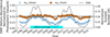 |
Fig. 1. SWE helium abundance in fast (filled marker) and slow (empty marker) wind intervals as a function of time, aggregated down to 250 days. The right axis plots the normalized 13-month smoothed sunspot number. The horizontal dotted line surrounded by the gray band indicating AHe = 51 ± 3% of its photospheric value is the weighted mean of the 250-day binned values along with the weighted uncertainty, where the weights are calculated as the standard deviation of AHe in each 250-day bin. |
2. Observations
In this study, we used the same dataset as in the Composition Saturation Paper. We combined observations of AHe from the Wind (Acuña et al. 1995) Solar Wind Experiment (SWE, Ogilvie et al. 1995) Faraday cups (FC) with heavy ion observations from the Advanced Composition Explorer (ACE, Stone et al. 1998) Solar Wind Ion Composition Spectrometer (SWICS, Gloeckler et al. 1998), a charge-resolving ion mass spectrometer. We used H and He observations available from the ACE Science Center (Garrard et al. 1998) using the same formulation as Lepri et al. (2013). A detailed discussion of the instruments are available in the cited papers. Both ACE and Wind observations are exclusively collected in the ecliptic plane. We used the 13-month smoothed sunspot number (SSN) to trace solar activity (SILSO World Data Center 2023). To calculate the normalized sunspot number (NSSN), we subtracted the minimum SSN during each cycle and then normalized this shifted SSN in a given cycle to its maximum value in that cycle. For solar cycle 25, we used a maximum SSN of 160.6, which is the prediction from NOAA’s Space Weather Prediction Testbed1.
3. Analysis
Figure 1 plots the SWE helium abundance as a function of time. The abundance has been split into fast and slow wind intervals, where the transition is defined by the speed vas 420 km s−1, at which the gradient of AHe as a function of vsw changes (Composition Saturation Paper). The interval over which SWICS observations are available is indicated at the bottom of the panel. Over the full time period plotted, the correlation coefficients between the SWE abundances and SSN are 0.94 (slow wind) and 0.66 (fast wind), both with p-values < 0.05. Using NSSN, we get 0.95 (slow wind) and 0.72 (fast wind) with p-values < 0.05. When only considering the time period for which SWICS observations are available, the correlation coefficients change to 0.95 (slow wind) and 0.75 (fast wind), again with p-values of < 0.05. Using NSSN, we get 0.95 (slow wind) and 0.76 (fast wind) with p-values < 0.05. These results are summarized in Table 1.
Correlation Coefficients between Abundances and SSN.
In Figure 1, the horizontal dotted line indicates AHe = 51 ± 3% with respect to the photospheric helium abundance, which is the weighted mean of the fast wind observations in the 250-day intervals. Here, the weights are calculated as the standard deviation of AHe in each 250-day interval and the gray band indicates the weighted uncertainty. The fast wind observations, which are predominantly from continuously open source regions, oscillate around half of the photospheric AHe. Slow wind AHe, which is predominantly from intermittently open source regions. It oscillates around a much larger range of values and reaches a maximum of this 51% level during solar maxima.
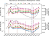 |
Fig. 2. SWICS abundances normalized to their photospheric values in (a) fast and (b) slow wind as a function of time, aggregated in 250-day intervals. The right axes plots the normalized 13-month smoothed sunspot number. The SWE abundances normalized to its photospheric values are plotted for reference. The vertical dotted lines indicate solar minimum 24. The vertical dash-dotted line indicates the helium shutoff (Alterman et al. 2021). |
Figure 2 plots the SWICS abundances as a function of time in (a) fast and (b) slow wind. In Figure 1, we calculate AHe as the simple average over the interval. In Figure 2, we calculate the weighted mean and standard error of the weighted mean because SWICS observations are reported with a 2 h cadence, instead of 92s by SWE. AHe derived from SWE observations is normalized to its photospheric value and plotted to show consistency with SWICS (He/H). The right axes indicate the normalized 13-month smoothed SSN. The vertical dotted lines indicate solar minimum 24. The vertical dash-dotted line indicate the helium shutoff preceding solar minimum 24. In general, there is a rough stratification in the abundances such that low FIP abundances are higher than high FIP abundances across the solar cycle. With the exception of slow wind S and fast wind Si, the observed minimum of fast wind (X/H):(X/H)photo precedes solar minimum 24 by 122 days and follows helium shutoff by 62 days.
To characterize the evolution of these abundances with solar activity, we calculated the correlation coefficient between each abundance and NSSN. For the SWE abundance, this is limited to the same time period over which the SWICS abundances are available. We also calculated the correlation coefficient between all SWICS abundances and the SWE abundance. These correlation coefficients are calculated for slow wind (vsw < vs) and fast wind (vsw > vs), where vs is defined as in Composition Saturation Paper for each species. As the SWE and SWICS data have a different observation cadence, the boundaries of each data set’s 250-day intervals do not necessarily overlap. As such, the SWE data have been interpolated to the SWICS observation time for this calculation. Table 1 summarizes these correlation coefficients for both slow and fast wind.
The SWE columns indicates the correlation coefficients between (X/H):(X/H)photo and AHe. The SSN columns indicate the correlation coefficients between a given abundance and SSN. Similarly, the NSSN column indicates the correlation coefficients between a given abundance and NSSN. Only significant correlation coefficients (p-value < 0.05) are shown. The correlation coefficient between fast and slow wind SWE abundances and SSN is stronger than the correlation between SWICS abundances and SSN. In general, the correlation coefficients derived for slow wind observations increase with increasing mass and (excluding C) all are strong (> 0.6 for SSN and > 0.7 for NSSN). In the fast wind, only four (SSN) or five (NSSN) of nine correlation coefficients using SWICS data are significant and none are strong (< 0.6); the exception is the correlation coefficient between (Fe/H):(Fe/H)photo and NSSN, which exceeds 0.6 and is thus significant. With the exception of slow wind Fe, SWICS (He/H):(He/H)photo is larger than all other (X/H):(X/H)photo correlation coefficients with SSN. Slow wind Fe ’s correlation coefficient with SSN is larger to slow wind He; its correlationcoefficient with NSSN in slow wind is equal to that of He. In fast wind, Fe exhibits the strongest correlation coefficient with SSN and NSSN. In the slow and fast wind, Fe exhibits the strongest correlation with AHe observed by SWE.
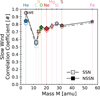 |
Fig. 3. Correlation coefficient between NSSN (solid line) or SSN (dash-dotted line) (X/H):(X/H)photo observed by ACE/SWICS along with AHe observed by Wind/SWE. With the exclusion of the helium abundances, the correlation coefficients monotonically increase with increasing M . All correlation coefficients using NSSN are stronger than those using SSN. |
Figure 3 plots the slow wind correlation coefficients with NSSN (solid line) and SSN (dash-dotted line) as a function of element mass (M). Markers are connected to aid the eye. The top axis identifies each species in the color corresponding to the marker and a vertical dotted line in the same color connects this label to the marker. The SWE abundance is labeled to differentiate it from the SWICS (He/H). As in Table 1, the correlation coefficients using NSSN are stronger than those using SSN. For elements heavier than He, we also observe a monotonic increase in the correlation strength with increasing mass. An ordering by charge state (Q), M/Q, and FIP is less apparent.
4. Discussion
Elemental abundances are set in the chromosphere and transition region. Because such quantities are fixed by the time the coronal plasma enters the solar wind, they serve as tracers of solar wind source regions and the physical processes active there. As such, the evolution of these abundances with solar activity is driven by the evolution of their solar sources. This work applies methods that have long been used to study the evolution of the solar wind helium abundances with solar activity (Aellig et al. 2001; Kasper et al. 2007, 2012; Alterman & Kasper 2019; Alterman et al. 2021; Yogesh et al. 2021) to heavy ion composition observations. To achieve sufficient statistical reliability in the observations, we did not split the observations into ten quantiles of vsw as has been done in prior work. Instead, we have split the solar wind into “slow” and “fast” regimes, where the different regimes are defined by speeds slower and faster than each species’ vs. This “saturation speed” (vs) is the speed at which the gradient of a given abundance as a function of vsw changes. The Composition Saturation Paper calculated vs values for heavy ion abundances observed by ACE/SWICS. When comparing vs for heavy abundances and AHe, we have noted them vas; Heavy and vasHe, respectively, to differentiate between the two. The Helium Saturation Paper applied the same method to Wind/FC observations of AHe. Based on the evolution of vs and the abundance at this speed (the saturation abundance As) with normalized cross helicity, the Helium Saturation Paper argued that “fast” wind (vsw > vs) primarily comes from polar solar source regions with magnetic topologies that are continuously open to the heliosphere and “slow” wind (vsw < vs) primarily comes from equatorial solar source regions with magnetic topologies that are only intermittently open to the heliosphere. The Composition Saturation Paper showed that (1) the gradient of (X/H):(X/H)photo and AHe for speeds vsw < vs are indistinguishable; (2) the heavy element saturation speeds is vs = 327 ± 2Heavy across all elements heavier than He; (3) vs > vasHe by 63 ± 4.5 km s−1; and (4) there is a mass- or charge-state- dependent fractionation of (X/H):(X/H)photo for speeds vsw > vs. From the first observation, the Composition Saturation Paper inferred that heavy element and He abundances are driven by the same process over speeds vsw < vs. From the second and third observations, they inferred that the process impacting (X/H):(X/H)photo and AHe for speeds vsw < vs takes place below heights at which vsw is established. Therefore, this is likely to occur in the chromosphere and/or transition region. These authors have argued that both of these results are consistent with gravitational settling. From the fourth observation, they identified a mass- or charge-state- dependent fractionation process that becomes increasingly significant with increasing speed; however, they provided no justification for this empirical observation.
4.1. SWE abundances
Figure 1 plots the solar wind helium abundance in two speed intervals: faster and slower than vs. The correlation coefficient between AHe and SSN in both speed intervals is high (> 0.6 or better). Alterman & Kasper (2019) analyzed AHe’s evolution with SSN across ten speed quantiles. The data in each quantile were aggregated into 250-day intervals. The slow wind interval defined in this work covers their seven slowest speed quantiles. Over these quantiles, the correlation coefficient between AHe and SSN exceeds 0.8. The fast wind interval defined in this work covers the three fastest speed intervals from Alterman & Kasper (2019) along with faster wind. This allowed us to extend the range of this analysis from a maximum of vsw ≈ 600 km s−1 to vsw ≈ 800 km s−1 (Aellig et al. 2001; Kasper et al. 2007, 2012; Alterman & Kasper 2019; Alterman et al. 2021). In these faster speed quantiles, the correlation coefficient between AHe and SSN markedly drops to below 0.7. These correlation coefficients likely exceed those reported by Kasper et al. (2007) across all speeds and those reported by Kasper et al. (2012) in faster quantiles because longer time intervals reduce the impact of fluctuations when calculating the correlation coefficients between two time series. This is, for example, why the two solar cycles of activity reported by Alterman & Kasper (2019) enabled the authors to characterize the vsw-dependent phase lag in the response of AHe to changes in the SSN. As such, although the speed intervals reported in this paper are markedly larger than those reported by Alterman & Kasper (2019), Kasper et al. (2007, 2012) and speeds vsw < vs aggregate over the speed-dependent phase lag between AHe and SSN (Alterman & Kasper 2019), the larger speed intervals in this paper are less sensitive to fluctuations in the aggregated values. This is likely why the correlation coefficient between AHe and SSN for speeds vsw < vs is closest to the strongest correlation coefficients reported for observations with speeds near the peak of the distribution of vsw observed near 1 AU (Kasper et al. 2007, 2012; Alterman & Kasper 2019). Regarding the speeds vsw > vs, the probability density of the distribution of vsw observed near 1 AU drops by nearly an order of magnitude from peak over the speed range 343 to ∼650 km s−1. Further dividing solar wind observations into smaller speed intervals increases the significance of random fluctuations in aggregated quantities. By aggregating across a wide range of speeds, we reduced the impact of such statistical fluctuations. This is why we are able to determine that AHe with speeds vsw > vs (and, thus, predominantly coming from source regions that are continuously open to the heliosphere) also evolves with solar activity. The fact that the correlation coefficients derived with NSSN exceed those derived with SSN in both the slow and fast wind indicates that the sunspot number is tracking the evolution of solar activity and not necessarily the physical process driving the evolution of AHe with it.
The photospheric helium abundance is 8.25 ± 0.2% (Asplund et al. 2021). For speeds vsw > vs, solar wind AHe oscillates around 51 ± 0.3% this value. During solar maximum, when solar wind sources with continuously open magnetic topologies (e.g., as coronal holes) are not confined to the Sun’s polar regions, solar wind AHe with speeds vsw < vs reaches a maximum during of 47.7% (maximum 24) to 49.7% (maximum 23) of its photospheric value. Given that coronal mass ejections (CMEs) release solar plasma from deep within the solar atmosphere and are known to be enhanced in heavy element abundances and AHe (e.g. Yogesh et al. 2022; Rivera et al. 2022b; Song et al. 2022), coupled with the fact that slow wind AHe is depleted from its fast wind values, we infer that the mechanism limiting non-transient solar wind AHe to ∼50% of its photospheric value occurs at heights near or below the chromosphere and transition region.
4.2. SWICS abundances
Per the Helium Saturation Paper and the Composition Saturation Paper, solar wind observations at 1 AU with vsw > vs predominantly come from source regions with magnetic field topologies that are continuously open to the heliosphere. In contrast, vsw < vs identifies solar wind that is predominantly from intermittently open source regions. We have divided (X/H):(X/H)photo observations into intervals with speeds above and below vs, where vs is calculated independently for each species (Composition Saturation Paper). Figure 2 plots each (X/H):(X/H)photo as a function of time aggregated in 250-day intervals. In this plot, we label vsw > vs as “fast wind” and vsw ≤ vs as “slow wind”. As expected, low FIP abundances are higher than high FIP abundances across the solar cycle.
According to Table 1, the correlation coefficients between SSN and these abundances is strong (> 0.6) and significant (p-value < 0.05) for all species in solar wind from intermittently open source regions. The Composition Saturation Paper showed that the gradients of (X/H):(X/H)photo as a function of vsw for vsw < vs are consistent across all species. This allows us to infer that the underlying physical mechanism is not preferentially coupled to any element. With the exception of He, Figure 3 shows that the correlation coefficient between SSN and (X/H):(X/H)photo with slow speeds from intermittently open source regions monotonically increases with increasing M.
It is unsurprising that He does not follow the trend in Figure 3. The Helium Saturation Paper argued that He is dynamically relevant for solar wind acceleration in both continuously and intermittently open source regions. This is likely why the correlation coefficient between AHe and SSN is strong and significant for both the vsw < vs and vsw > vs speed ranges. In contrast, heavy element abundances are likely too small to be dynamically relevant to the solar plasma’s overall acceleration into the solar wind.
The similarity in the correlation coefficients of SSN with (X/H):(X/H)photo and AHe for vsw < vs suggests that one or more processes drive the long term evolution of these abundances in similar ways. This is reflected in the correlation coefficients between AHe and (X/H):(X/H)photo in that they are (with the exception of C) strong and significant in slow wind with vsw < vs and either weak (< 0.6) or insignificant (high p-value > 0.05) in fast wind with vsw > vs. The fact that the correlation coefficients derived with NSSN exceed those derived with SSN further suggests that the sunspot number is a “clock” for timing solar activity, but it does not trace the underlying process driving the evolution of (X/H):(X/H)photo.
Gravitational settling is one process that governs abundances in closed loops that is coupled to elements based on their mass, not their charge state, FIP, Q/M, and so on (Vauclair & Charbonnel 1991; Borrini et al. 1981; Hirshberg 1973; Weberg et al. 2015; Alterman & Kasper 2019). Such loops are longer lived during solar minima, leading to more depleted abundances. This mechanism does not affect solar wind from continuously open source regions where such closed loops are absent. As such, we infer that the difference between the evolution with solar activity of solar wind abundances from continuously and intermittently open source regions may be driven by gravitational settling in such regions.
That the correlation coefficient between slow wind AHe and SSN is higher than the heavier elements may signify that the evolution of helium with solar activity is driven by additional processes (e.g., the Helium Saturation Paper, and references there in) that do not couple to heavier elements. Figure 7 in the Composition Saturation Paper shows that vs; HeHeavy + 63 km s−1 and these two speeds are separated by the peak of the solar wind speed distribution, further suggesting that some other process is accelerating He to faster speeds than heavy elements. However, we cannot rule out that the 2-h duration of SWICS measurements means that we cannot separate solar wind by speed when vsw ∼ vs for SWICS observations with the same precision as we can for SWE observations and that only one solar cycle of SWICS observations means that statistical fluctuations have a more significant impact on our SWICS observations than our SWE observations for vsw > vs
4.3. Composition shutoff
The time between the observed minimum in fast wind (X/H):(X/H)photo and the helium shutoff preceding solar minimum 24 (Alterman et al. 2021) is half as long as the time between the minimum in fast wind (X/H):(X/H)photo and solar minimum 24. However, both of these intervals are within the 250-day averaging window and the 229-day uncertainty in the helium shutoff. As such, any inference from this observation requires higher time resolution analysis.
4.4. Drivers of the helium and heavy element abundances
McIntosh et al. (2011) studied how the relationship between AHe, the iron-to-oxygen ratio (Fe/O), adverage iron charge state (⟨Q⟩), and characteristic scale size in the transition region evolve with solar activity in slow (vsw < 400 km s−1) and fast (vsw > 500 km s−1) solar wind. They argue that the drop in AHe during solar minima is consistent with a decrease in the energy available to accelerate coronal helium into the solar wind during this phase of solar activity. They suggested that this is consistent with a decrease in the transition regions scale size during solar minima, which also implies less energy available to heat the solar wind at these heights, resulting in a reduced number density (McComas et al. 2008) and ⟨Q⟩. This depletion in available energy is consistent with observations of solar wind O7+/O6+ and C6+/C5+] charge state ratios that evolve with SSN and drop during solar minima (Kasper et al. 2012). Given that coronal electron temperatures and densities likely do not change with solar activity (Landi & Testa 2014) and that the efficiency of solar wind acceleration likely varies with source regions, the evolution of these parameters with solar activity likely reflects the evolution of the frequency at which solar wind from different source regions is sampled at 1 AU.
In the case of fast wind, the solar wind originates from continuously open source regions with radial magnetic fields. In such solar wind, AHe and heavy ion abundances do not vary significantly because the solar wind primarily originates from a single class of source region.
In the case of slow wind, Kasper et al. (2012) attributed the variability of AHe to the occurrence of two different sources. One is ARs, the edge of which recent studies suggest may be consistent with sources of the Alfvénic slow wind (Baker et al. 2023; Yardley et al. 2024; Ervin et al. 2024b). The other is the streamer belt. Alterman & Kasper (2019) argued that the vsw-dependent phase lag in the response of AHe to changes in SSN for speeds vsw ≤ 574 km s−1 is consistent with a He filtration mechanism. When set in the context of the results from the Helium Saturation Paper, such a filtration mechanism may be related to the energy available to accelerate coronal helium into the solar wind, which varies with the source region (Hansteen et al. 1997; Endeve et al. 2005). Such an inference is consistent with Yogesh et al. (2021), who argued that this filtration mechanism is related to the topology of the Sun’s magnetic field. If the heat flux mediated coupling between the corona and transition region is significant for determining the energy available to accelerate the solar wind or, equivalently, the acceleration efficiency (Lie-Svendsen et al. 2001, 2002), such an inference is also consistent with differences between fast wind being “generated in the low corona, where C and O freeze-in, and then the two winds experience a similar evolution in the extended corona, where Fe freezes-in” (Lepri et al. 2013). If this is indeed the case, the highly variable X/H in solar wind with vsw < vs also reflects the energy available to accelerate heavy ions from the solar plasma into the solar wind. The vsw-dependent filtration mechanism may be related to helium’s dynamic role in solar wind acceleration (Hansteen et al. 1997; Endeve et al. 2005; Alterman & D’Amicis 2025), for which heavy element abundances are too small.
5. Conclusion
We have observed the evolution of the solar wind helium abundance and heavy element abundances with solar activity. The helium abundance observations cover approximately 22 years of Wind/SWE operations, while the abundances of heavier elements are limited to approximately 12 years during ACE/SWICS operations prior to the detector degradation. Using the solar wind helium abundance, we have made the following observations:
-
AHe observed in slow and fast wind is strongly correlated with the Sun’s activity cycle, as observed in SSN data.
-
The correlation coefficients derived with the normalized SSN (NSSN) are stronger than those derived with SSN, indicating that the sunspot number is a “clock” timing the evolution of solar activity, not the underlying physical process that modulates AHe.
-
Solar wind helium in fast wind, which is predominantly from continuously open magnetic sources, oscillates around 51% of its photospheric value.
-
In slow wind from intermittently open source regions, AHe is highly variable below 51% and only reaches this maximum value during solar maxima when continuously and intermittently open source regions are not confined to the Sun’s polar regions.
Using heavy ion abundances from ACE/SWICS, we have made the following observations:
-
In slow wind, the abundance of all heavy elements except C is strongly correlated with SSN.
-
In fast wind, (X/H):(X/H)photo abundances do not evolve significantly with solar activity. However, the more periods of oscillation observed, the less significant the impact any random fluctuations would have on the correlation coefficient. Because (a) we have more than two solar activity cycles from AHe observations and our observations of (X/H):(X/H)photo cover a time period slightly longer than one solar activity cycle and (b) fast wind oscillations are smaller in amplitude than slow wind oscillations, we cannot conclusively state that this is because (X/H):(X/H)photo in fast wind does not evolve with solar activity. Alternatively, the result could be due to the limited duration of our heavy ion observations.
-
The correlation coefficients derived between (X/H):(X/H)photo and NSSN are stronger than those derived with SSN, further indicating that the sunpot number is tracking solar activity, but not the underlying process that drives the evolution of the abundances.
-
Unsurprisingly, the strong correlation between AHe and SSN along with (X/H):(X/H)photo and SSN is reflected in a strong correlation between AHe and (X/H):(X/H)photo. That these correlation coefficients are weaker is unsurprising because we use the 13-month smoothed SSN and neither the 250-day average AHe nor (X/H):(X/H)photo are smoothed.
-
The correlation coefficients between (X/H):(X/H)photo and SSN monotonically increase with increasing element mass. We infer that this is a signature of gravitational settling in slow wind, which is consistent with the gradient of (X/H):(X/H)photo over speeds vsw < vs being indistinguishable across the heavier elements (Composition Saturation Paper).
-
The helium shutoff is a precipitous depletion and recovery in AHe that precedes SSN minima by approximately 229 days (Alterman et al. 2021). The largest source of uncertainty on this observation is the 250-day averaging window. The minimum (X/H):(X/H)photo we observed precedes SSN minima by 122 days, but follows the helium shutoff by only 62 days. In other words, the time between the minimum in (X/H):(X/H)photo and the helium shutoff is half as long as the time between the minimum (X/H):(X/H)photo and SSN minima. However, the difference between these two times is smaller than the 229-day uncertainty on helium shutoff and the 250-day averaging window. As such, higher time-resolution analysis is necessary to determine if the depletion of (X/H):(X/H)photo during solar minima coincides with helium shutoff.
We attribute the differences between the evolution of AHe and (X/H):(X/H)photo in slow wind with solar activity to helium’s dynamic involvement in solar wind acceleration (Helium Saturation Paper, and references therein). These differences are also reflected in the difference between vs for He and heavier elements derived in the Composition Saturation Paper. The differences in fast wind are either also related to how helium is dynamically relevant for solar wind acceleration or simply driven by the lower SWICS data volume with respect to SWE. More broadly, we infer that the variation in both AHe and (X/H):(X/H)photo with solar activity is driven by the energy in the chromosphere and transition region or low corona, which is also related to the topology of the magnetic field in the solar wind’s source regions. This suggests that the evolution of slow wind AHe and (X/H):(X/H)photo with solar activity observed at 1 AU may be due to changes in the frequency of observing solar wind from different source regions.
In closing, we note that both ACE’s and Wind’s orbits are in the ecliptic plane. Given that the occurrence rate and heliographic latitude of different solar source regions changes with solar activity, long-duration out-of-ecliptic observations are necessary to fully understand the relationship between source region and in situ abundances. Furthermore, recent results show that Alfvén wave energy deposition (Rivera et al. 2025; Alterman 2025) and thermal pressure gradients (Rivera et al. 2024) accelerate the solar wind in transit through interplanetary space. This means such out-of-ecliptic observations need to be either collected over a long duration and at a single radial distance or the relevant in situ acceleration mechanisms must be well understood so that radial gradients in vsw can be properly accounted for; for instance, with observations from Ulysses/SWICS (Gloeckler et al. 1992; von Steiger et al. 2000). This approach would allow us to properly trace in situ observations back to their source regions and such observations are a critical component of future missions (Rivera & Badman 2025).
Acknowledgments
BLA thanks F. Carcaboso for helpful discussions about the helium abundance variation with time. BLA acknowledges funding from NASA Grants 80NSSC22K0645 (LWS/TM) and 80NSSC22K1011 (LWS). JMR and STL acknowledge NASA contract 80NSSC23K0542 (ACE/SWICS). Sunspot data from the World Data Center SILSO, Royal Observatory of Belgium, Brussels. The authors thank the referee for their useful questions and helpful suggestions.
References
- Abbo, L., Ofman, L., Antiochos, S. K., et al. 2016, Space Sci. Rev., 201, 55 [NASA ADS] [CrossRef] [Google Scholar]
- Acuña, M. H., Ogilvie, K. W., Baker, D. N., et al. 1995, Space Sci. Rev., 71, 5 [Google Scholar]
- Aellig, M. R., Lazarus, A. J., & Steinberg, J. T. 2001, GRL, 28, 2767 [NASA ADS] [CrossRef] [Google Scholar]
- Alterman, B. 2025, ApJ, 984, L64 [Google Scholar]
- Alterman, B. L., & D’Amicis, R. 2025, ApJ, 982, L40 [Google Scholar]
- Alterman, B. L., & Kasper, J. C. 2019, ApJ, 879, L6 [Google Scholar]
- Alterman, B. L., Kasper, J. C., Stevens, M., & Koval, A. 2018, ApJ, 864, 112 [NASA ADS] [CrossRef] [Google Scholar]
- Alterman, B. L., Kasper, J. C., Leamon, R. J., & McIntosh, S. W. 2021, Sol. Phys., 296, 67 [Google Scholar]
- Alterman, B. L., Rivera, Y. J., Lepri, S. T., & Raines, J. M. 2025, A&A, 694, A265 [NASA ADS] [CrossRef] [EDP Sciences] [Google Scholar]
- Antiochos, S. K., Mikic, Z., Titov, V. S., Lionello, R., & Linker, J. A. 2011, ApJ, 731, 112 [NASA ADS] [CrossRef] [Google Scholar]
- Antonucci, E., Abbo, L., & Dodero, M. A. 2005, A&A, 435, 699 [NASA ADS] [CrossRef] [EDP Sciences] [Google Scholar]
- Asplund, M., Amarsi, A. M., & Grevesse, N. 2021, A&A, 653, A141 [NASA ADS] [CrossRef] [EDP Sciences] [Google Scholar]
- Baker, D., Démoulin, P., Yardley, S. L., et al. 2023, ApJ, 950, 65 [CrossRef] [Google Scholar]
- Berger, L., Wimmer-Schweingruber, R. F., & Gloeckler, G. 2011, Phys. Rev. Lett., 106, 151103 [NASA ADS] [CrossRef] [Google Scholar]
- Borrini, G., Gosling, J. T., Bame, S. J., et al. 1981, J. Geophys. Res.: Space Phys., 86, 4565 [Google Scholar]
- Brooks, D. H., Ugarte-Urra, I., & Warren, H. P. 2015, Nat. Commun., 6, 5947 [Google Scholar]
- Bruno, R., & Carbone, V. 2013, Liv. Rev. Sol. Phys., 10, 1 [Google Scholar]
- Crooker, N. U., Antiochos, S. K., Zhao, X., & Neugebauer, M. 2012, J. Geophys. Res.: Space Phys., 117, A04104 [Google Scholar]
- D’Amicis, R., & Bruno, R. 2015, ApJ, 805, 1 [NASA ADS] [CrossRef] [Google Scholar]
- D’Amicis, R., Bruno, R., & Bavassano, B. 2011, J. Atmos. Sol.-Terr. Phys., 73, 653 [CrossRef] [Google Scholar]
- D’Amicis, R., Bruno, R., & Matteini, L. 2016, AIP Conf. Proc., 1720, 040002 [Google Scholar]
- D’Amicis, R., Matteini, L., & Bruno, R. 2018, MNRAS, 14, 1 [Google Scholar]
- D’Amicis, R., Perrone, D., Bruno, R., & Velli, M. 2021a, J. Geophys. Res.: Space Phys., 126, e28996 [Google Scholar]
- D’Amicis, R., Alielden, K., Perrone, D., et al. 2021b, A&A, 654, A111 [NASA ADS] [CrossRef] [EDP Sciences] [Google Scholar]
- Ďurovcová, T., Šafránková, J., & Němeček, Z. 2019, Sol. Phys., 294, 97 [CrossRef] [Google Scholar]
- Elsasser, W. M. 1950, Phys. Rev., 79, 183 [Google Scholar]
- Endeve, E., Lie-Svendsen, O., Hansteen, V. H., & Leer, E. 2005, ApJ, 624, 402 [NASA ADS] [CrossRef] [Google Scholar]
- Ervin, T., Bale, S. D., Badman, S. T., et al. 2024a, ApJ, 969, 83 [Google Scholar]
- Ervin, T., Jaffarove, K., Badman, S. T., et al. 2024b, ApJ, 975, 156 [NASA ADS] [CrossRef] [Google Scholar]
- Feldman, W. C., Asbridge, J. R., Bame, S. J., & Gosling, J. T. 1978, JGR, 83, 2177 [Google Scholar]
- Fisk, L. A., Zurbuchen, T. H., & Schwadron, N. A. 1999, ApJ, 521, 868 [Google Scholar]
- Fu, H., Li, B., Li, X., et al. 2015, Sol. Phys., 290, 1399 [CrossRef] [Google Scholar]
- Fu, H., Madjarska, M. S., Xia, L., et al. 2017, ApJ, 836, 169 [Google Scholar]
- Garrard, T., Davis, A. J., Hammond, J., & Sears, S. 1998, Space Sci. Rev., 86, 649 [Google Scholar]
- Geiss, J. 1982, Space Sci. Rev., 33, 201 [Google Scholar]
- Geiss, J., Gloeckler, G., & von Steiger, R. 1995a, Space Sci. Rev., 72, 49 [NASA ADS] [CrossRef] [Google Scholar]
- Geiss, J., Gloeckler, G., Von Steiger, R., et al. 1995b, Science, 268, 1033 [CrossRef] [Google Scholar]
- Gloeckler, G., Geiss, J., Balsiger, H., et al. 1992, A&AS, 92, 267 [NASA ADS] [Google Scholar]
- Gloeckler, G., Cain, J., Ipavich, F. M., et al. 1998, Space Sci. Rev., 86, 497 [NASA ADS] [CrossRef] [Google Scholar]
- Grappin, R., Velli, M., & Mangeney, A. 1991, Ann. Geophys., 9, 416 [Google Scholar]
- Hansteen, V. H., Leer, E., & Holzer, T. E. 1997, ApJ, 482, 498 [Google Scholar]
- Hirshberg, J. 1973, Astrophys. Space Sci., 20, 473 [Google Scholar]
- Kasper, J. C., Lazarus, A. J., Steinberg, J. T., Ogilvie, K. W., & Szabo, A. 2006, JGR, 111, A03105 [Google Scholar]
- Kasper, J. C., Stevens, M., Lazarus, A. J., Steinberg, J. T., & Ogilvie, K. W. 2007, ApJ, 660, 901 [NASA ADS] [CrossRef] [Google Scholar]
- Kasper, J. C., Lazarus, A. J., & Gary, S. P. 2008, Phys. Rev. Lett., 101, 261103 [Google Scholar]
- Kasper, J. C., Stevens, M. L., Korreck, K. E., et al. 2012, ApJ, 745, 162 [Google Scholar]
- Kasper, J. C., Klein, K. G., Weber, T., et al. 2017, ApJ, 849, 126 [NASA ADS] [CrossRef] [Google Scholar]
- Klein, K. G., Verniero, J. L., Alterman, B. L., et al. 2021, ApJ, 909, 7 [NASA ADS] [CrossRef] [Google Scholar]
- Laming, J. M. 2004, ApJ, 614, 1063 [Google Scholar]
- Laming, J. M. 2009, ApJ, 695, 954 [NASA ADS] [CrossRef] [Google Scholar]
- Laming, J. M. 2015, Liv. Rev. Sol. Phys., 12, 2 [Google Scholar]
- Landi, E., & Testa, P. 2014, ApJ, 787, 33 [Google Scholar]
- Lepri, S. T., & Rivera, Y. J. 2021, ApJ, 912, 51 [NASA ADS] [CrossRef] [Google Scholar]
- Lepri, S. T., Landi, E., & Zurbuchen, T. H. 2013, ApJ, 768, 94 [NASA ADS] [CrossRef] [Google Scholar]
- Lie-Svendsen, O., Leer, E., & Hansteen, V. H. 2001, J. Geophys. Res.: Space Phys., 106, 8217 [Google Scholar]
- Lie-Svendsen, O., Hansteen, V. H., Leer, E., & Holzer, T. E. 2002, ApJ, 566, 562 [Google Scholar]
- Marsch, E., & Tu, C.-Y. Y. 1990, Journal of Geophysical Research, 95, 8211 [Google Scholar]
- Marsch, E., Mühlhäuser, K.-H., Rosenbauer, H., Schwenn, R., & Denskat, K. U. 1981, JGR, 86, 9199 [Google Scholar]
- McComas, D. J., Ebert, R. W., Elliott, H. A., et al. 2008, GRL, 35, L18103 [Google Scholar]
- McIntosh, S. W., Kiefer, K. K., Leamon, R. J., Kasper, J. C., & Stevens, M. 2011, ApJ, 740, 1 [Google Scholar]
- Ogilvie, K. W., Chornay, D. J., Fritzenreiter, R. J., et al. 1995, Space Sci. Rev., 71, 55 [Google Scholar]
- Phillips, J. L., Balogh, A., Bame, S. J., et al. 1994, GRL, 21, 1105 [Google Scholar]
- Rakowski, C. E., & Laming, J. M. 2012, ApJ, 754, 65 [Google Scholar]
- Rivera, Y. J., & Badman, S. T. 2025, arXiv e-prints [arXiv:2502.06036] [Google Scholar]
- Rivera, Y. J., Higginson, A., Lepri, S. T., et al. 2022a, Front. Astron. Space Sci., 9, 1056347 [CrossRef] [Google Scholar]
- Rivera, Y. J., Raymond, J. C., Landi, E., et al. 2022b, ApJ, 936, 83 [NASA ADS] [CrossRef] [Google Scholar]
- Rivera, Y. J., Badman, S. T., Stevens, M. L., et al. 2024, Science, 385, 962 [NASA ADS] [CrossRef] [Google Scholar]
- Rivera, Y. J., Badman, S. T., Verniero, J. L., et al. 2025, ApJ, 980, 70 [Google Scholar]
- Schwadron, N. A., Fisk, L. A., & Zurbuchen, T. H. 1999, ApJ, 521, 859 [Google Scholar]
- SILSO World Data Center 2023, http://sidc.oma.be/silso/ [Google Scholar]
- Song, H., Cheng, X., Li, L., Zhang, J., & Chen, Y. 2022, ApJ, 925, 137 [Google Scholar]
- Stakhiv, M. O., Lepri, S. T., Landi, E., Tracy, P. J., & Zurbuchen, T. H. 2016, ApJ, 829, 117 [NASA ADS] [CrossRef] [Google Scholar]
- Stone, E. C., Frandsen, A. M., Mewaldt, R. A., et al. 1998, Space Sci. Rev., 86, 1 [Google Scholar]
- Subramanian, S., Madjarska, M. S., & Doyle, J. G. 2010, A&A, 516, A50 [NASA ADS] [CrossRef] [EDP Sciences] [Google Scholar]
- Tracy, P. J., Kasper, J. C., Zurbuchen, T. H., et al. 2015, ApJ, 812, 170 [NASA ADS] [CrossRef] [Google Scholar]
- Tracy, P. J., Kasper, J. C., Raines, J. M., et al. 2016, Phys. Rev. Lett., 255101, 255101 [CrossRef] [Google Scholar]
- Tu, C. Y., & Marsch, E. 1995, Space Sci. Rev., 73, 1 [Google Scholar]
- Tu, C.-Y., Marsch, E., & Thieme, K. M. 1989, JGR, 94, 11739 [Google Scholar]
- Vauclair, S., & Charbonnel, C. 1991, Challenges to Theories of the Structure of Moderate-Mass Stars (Berlin, Heidelberg: Springer), 37 [Google Scholar]
- Verniero, J. L., Larson, D. E., Livi, R., et al. 2020, ApJS, 248, 5 [Google Scholar]
- Verniero, J. L., Chandran, B. D. G., Larson, D. E., et al. 2022, ApJ, 924, 112 [NASA ADS] [CrossRef] [Google Scholar]
- von Steiger, R., Schwadron, N. A., Fisk, L. A., et al. 2000, J. Geophys. Res.: Space Phys., 105, 27217 [Google Scholar]
- Weberg, M., Lepri, S. T., & Zurbuchen, T. H. 2015, ApJ, 801, 1 [NASA ADS] [CrossRef] [Google Scholar]
- Woodham, L. D., Wicks, R. T., Verscharen, D., & Owen, C. J. 2018, ApJ, 856, 49 [CrossRef] [Google Scholar]
- Xu, F., & Borovsky, J. 2015, J. Geophys. Res.: Space Phys., 120, 70 [NASA ADS] [CrossRef] [Google Scholar]
- Yardley, S. L., Brooks, D. H., D’Amicis, R., et al. 2024, Nat. Astron., 8, 953 [NASA ADS] [CrossRef] [Google Scholar]
- Yogesh, Chakrabarty, D., & Srivastava, N. 2021, MNRAS, 503, L17 [NASA ADS] [CrossRef] [Google Scholar]
- Yogesh, Chakrabarty, D., & Srivastava, N. 2022, MNRAS, 111, 106 [Google Scholar]
- Zhao, L., Landi, E., & Gibson, S. E. 2013, ApJ, 773, 157 [Google Scholar]
- Zhao, L., Landi, E., Lepri, S. T., et al. 2017, ApJ, 846, 135 [Google Scholar]
- Zhao, L., Landi, E., Lepri, S. T., & Carpenter, D. 2022, Universe, 8, 393 [NASA ADS] [CrossRef] [Google Scholar]
- Zurbuchen, T. H., Weberg, M., Von Steiger, R., et al. 2016, ApJ, 826, 10 [CrossRef] [Google Scholar]
All Tables
All Figures
|
Fig. 1. SWE helium abundance in fast (filled marker) and slow (empty marker) wind intervals as a function of time, aggregated down to 250 days. The right axis plots the normalized 13-month smoothed sunspot number. The horizontal dotted line surrounded by the gray band indicating AHe = 51 ± 3% of its photospheric value is the weighted mean of the 250-day binned values along with the weighted uncertainty, where the weights are calculated as the standard deviation of AHe in each 250-day bin. |
| In the text | |
|
Fig. 2. SWICS abundances normalized to their photospheric values in (a) fast and (b) slow wind as a function of time, aggregated in 250-day intervals. The right axes plots the normalized 13-month smoothed sunspot number. The SWE abundances normalized to its photospheric values are plotted for reference. The vertical dotted lines indicate solar minimum 24. The vertical dash-dotted line indicates the helium shutoff (Alterman et al. 2021). |
| In the text | |
|
Fig. 3. Correlation coefficient between NSSN (solid line) or SSN (dash-dotted line) (X/H):(X/H)photo observed by ACE/SWICS along with AHe observed by Wind/SWE. With the exclusion of the helium abundances, the correlation coefficients monotonically increase with increasing M . All correlation coefficients using NSSN are stronger than those using SSN. |
| In the text | |
Current usage metrics show cumulative count of Article Views (full-text article views including HTML views, PDF and ePub downloads, according to the available data) and Abstracts Views on Vision4Press platform.
Data correspond to usage on the plateform after 2015. The current usage metrics is available 48-96 hours after online publication and is updated daily on week days.
Initial download of the metrics may take a while.