| Issue |
A&A
Volume 700, August 2025
|
|
|---|---|---|
| Article Number | A73 | |
| Number of page(s) | 7 | |
| Section | Stellar structure and evolution | |
| DOI | https://doi.org/10.1051/0004-6361/202554341 | |
| Published online | 05 August 2025 | |
The properties of supermassive stars in galaxy merger-driven direct collapse
I. Models without rotation
Département d’Astronomie, Université de Genève, Chemin Pegasi 51, CH-1290 Versoix, Switzerland
⋆ Corresponding author.
Received:
1
March
2025
Accepted:
23
June
2025
Abstract
Context. The formation of the most massive quasars observed at high redshifts requires extreme accretion rates (> 1 M⊙ yr−1). Inflows of 10−1000 M⊙ yr−1 are found in hydrodynamical simulations of galaxy mergers, leading to the formation of supermassive discs (SMDs) with high metallicities (> Z⊙). Supermassive stars (SMSs) born in these SMDs could be the progenitors of the most extreme quasars.
Aims. Here, we study the properties of non-rotating SMSs forming in high-metallicity SMDs.
Methods. Using the stellar evolution code GENEC, we carried out a numerical computation of the hydrostatic structures of non-rotating SMSs with metallicities of Z = 1 − 10 Z⊙ by following their evolution under constant accretion at rates of 10−1000 M⊙ yr−1. We determined the final mass of the SMSs, set by general-relativistic (GR) instability, by applying the relativistic equation of adiabatic pulsations to the hydrostatic structures.
Results. We find that non-rotating SMSs with metallicities of Z = 1 − 10 Z⊙ and accreting at rates of 10−1000 M⊙ yr−1 evolve as red supergiant protostars until their final collapse. All the models reach the GR instability during H-burning. The final mass is ∼106 M⊙ and this result is found to be nearly independent of the metallicity and the accretion rate.
Key words: stars: black holes / stars: massive
© The Authors 2025
 Open Access article, published by EDP Sciences, under the terms of the Creative Commons Attribution License (https://creativecommons.org/licenses/by/4.0), which permits unrestricted use, distribution, and reproduction in any medium, provided the original work is properly cited.
This article is published in open access under the Subscribe to Open model. This email address is being protected from spambots. You need JavaScript enabled to view it. to support open access publication.
1. Introduction
In the last decade, a number of quasars hosting supermassive black holes (SMBHs) with masses of 106 − 109 M⊙ have been discovered at redshifts of z ≳ 7 (Wu et al. 2015; Bañados et al. 2018; Wang et al. 2018, 2021; Yang et al. 2020; Larson et al. 2023; Kokorev et al. 2023; Kovács et al. 2024; Bogdán et al. 2024; Maiolino et al. 2024). The young age of the Universe at these redshifts implies an extremely rapid formation process for these SMBHs (Woods et al. 2019; Haemmerlé et al. 2020). One promising scenario is direct collapse, namely, the direct formation of a SMBH seed with a mass of ≳105 − 106 M⊙. In this scenario, the progenitor of the SMBH seed is a supermassive star (SMS) growing by accretion (Hosokawa et al. 2012, 2013; Umeda et al. 2016; Woods et al. 2017, 2021, 2024; Haemmerlé et al. 2018a,b, 2019; Herrington et al. 2023; Nandal et al. 2023, 2024) until it reaches the general-relativistic (GR) instability (Chandrasekhar 1964; Haemmerlé 2020, 2021a,b; Haemmerlé 2024; Saio et al. 2024; Nagele & Umeda 2024).
Direct collapse requires special conditions. In the collapse of an isolated primordial halo, molecular cooling by H2 is found to limit the sellar mass to ∼100 M⊙ (e.g. Bromm et al. 2002; Klessen & Glover 2023). In the presence of a strong Lyman-Werner flux, which dissociates H2, a zero-metallicity SMS can form, under accretion at rates 0.01−1 M⊙ yr−1, in the collapse of the atomically cooled halo (e.g. Haiman et al. 1997; Omukai 2001; Dijkstra et al. 2008; Bromm & Loeb 2003; Latif et al. 2013; Regan et al. 2017; Chon et al. 2018). Alternatively, supersonic baryon motions relative to dark matter can also produce pristine 107 M⊙ halos and SMSs with similar accretion rates (e.g. Schauer et al. 2017; Woods et al. 2017).
Another channel of direct collapse is the case of the merger of massive gas-rich galaxies (Mayer et al. 2010, 2015, 2024; Zwick et al. 2023). In this scenario, inflows of 10−1000 M⊙ yr−1 are triggered down to parsec scales (see Figure 5 of Mayer et al. 2024), which results in the formation of a rotationally supported supermassive disc (SMD) with mass ∼109 M⊙. Cosmological simulations indicate that such SMDs are metal-rich, with a metallicity value in the range of 1−10 Z⊙, typically 3 Z⊙ (see Figure 7 of Mayer et al. 2024).
SMSs with high metallicities have been studied by Appenzeller & Fricke (1972a,b), Fuller et al. (1986), Montero et al. (2012), Haemmerlé et al. (2019), and Nagele & Umeda (2024). Among these works, only Haemmerlé et al. (2019) and Nagele & Umeda (2024) accounted for accretion, assuming metallicities up to solar. Appenzeller & Fricke (1972a,b) studied the collapse of non-accreting, non-rotating SMSs with masses of 520 000 M⊙ and 750 000 M⊙, at metallicities of Z = 0.03. They found that the most massive star collapses into a SMBH, while the less massive one explodes because of the hot CNO cycle. Fuller et al. (1986) showed that non-accreting, non-rotating SMSs with masses of 105 − 106 M⊙ explode as soon as their metallicity exceeds Z ≳ 0.005. Montero et al. (2012) showed that rotation decreases the threshold metallicity for explosions down to 0.001.
We study, for the first time, the properties of SMSs forming by accretion in the conditions of galaxy merger-driven direct collapse, that is, with metallicities of > Z⊙ and accretion rates of 10−1000 M⊙ yr−1. We numerically derived the properties of such SMSs during their hydrostatic accretion phase, as well as their final masses at collapse, set by the GR instability, which provides an estimate of the mass of the SMBH seeds formed in this scenario. This work is the first of a series and we considered only the non-rotating case. The method is described in Sect. 2, while the results are presented in Sect. 3 and discussed in Sect. 4. We present our conclusions in Sect. 5.
2. Method
2.1. Hydrostatic structures
The hydrostatic structures were computed with GENEC (Eggenberger et al. 2008), a one-dimensional hydrostatic stellar evolution code that numerically solves the equations of stellar structure with the Henyey method. The code includes the GR Tolman-Oppenheimer-Volkoff corrections to hydrostatic equilibrium in the post-Newtonian approximation (Haemmerlé et al. 2018a). Accretion is included under the assumption of cold accretion (Haemmerlé et al. 2016). We started from an initial model of M = 100 M⊙ and considered constant accretion at rates of Ṁ = 10−100−1000 M⊙ yr−1. We used such a high initial mass because the rates considered are not consistent with gravity for lower masses (Haemmerlé et al. 2021). Moreover, as shown in Haemmerlé et al. (2019), for such rapid accretion, hydrostatic equilibrium is not guaranteed for M ≲ 104 M⊙. However, for M ≳ 100 M⊙, most of the stellar mass would be expected to reach hydrostatic equilibrium and only the outer envelope might then evolve hydrodynamically (see Figure 3 of Haemmerlé et al. 2019).
The chemical composition of the initial model and that of the accreted material are identical and scaled with the solar abundances of Asplund et al. (2005). For each metallicity, Z = 1 − 3 − 10 Z⊙, the mass fraction of hydrogen (X) and of helium (Y) are set by extrapolation from the primordial and solar compositions,
 (1)
(1)
 (2)
(2)
where Y0 = 0.2484 is the primordial helium mass fraction.
The reactions network includes the burning of light elements, the pp-chain, and the cold CNO cycle, which involves 21 isotopes. The hot CNO cycle is not included, as the central temperature remains < 108 K (Figure 3).
2.2. GR instability
We determined the GR instability point with the method of Chandrasekhar (1964). This method relies on a linear pulsation analysis of Einstein’s field equations in spherical symmetry, assuming adiabatic perturbations to equilibrium. The pulsation equation is expressed as
 (3)
(3)
where ′ denotes a derivative with respect to the radial coordinate r, ω is the pulsation frequency, ξ the radial displacement of the perturbation, Γ1 the first adiabatic exponent, P the thermal pressure, ρ the relativistic mass density, c the speed of light, G the gravitational constant, and a and b are the coefficients of the metric:
 (4)
(4)
Except for ω and ξ, all the quantities involved in Equation (3) refer to equilibrium.
Equation (3) is an eigenvalue problem, where we have
 (5)
(5)
for the Sturm-Liouville operator
 (6)
(6)
with f(r) = r2e−aξ(r) and the boundary conditions ξ(0) = 0 and δP(R) = 0. The operator ℒ is self-adjoint for the scalar product,
 (7)
(7)
As a consequence, the spectral theorem implies that there an orthonormal basis (of the real vector space of functions satisfying the required boundary conditions) exists, whose elements are the eigenvectors of ℒ. In other words, any function, f(r), that satisfies the required boundary conditions can be written as a linear combination of eigenfunctions, fi, with an eigenvalue, λi, namely,
 (8)
(8)
Furthermore, the different fi values are all orthonormal to each other. Thus, it is implied that
 (9)
(9)
We can see that if there is any function f(r) whose scalar product with its image through ℒ is negative, then there is necessarily at least one negative eigenvalue, λi < 0. Indeed, if the left-hand side of Equation (9) is negative, the right-hand side must also be negative, which is possible only if one of the λi values is negative. And if an eigenvalue of ℒ is negative, it implies that there are solutions to Equation (3) with an imaginary pulsation frequency and thereby indicating that the star is GR unstable.
By applying the scalar product ⟨f|⋅⟩ with f(r) = r2e−aξ(r) on the two sides of Equation (3), we obtain
 (10)
(10)
We can transform the first term on the right-hand side by an integration by parts (where the boundary terms vanish) and we obtain
 (11)
(11)
This is equivalent to Equation (61) of Chandrasekhar (1964). This corresponds to
 (12)
(12)
And as we see from Equation (9), a sufficient condition for GR instability is that the right-hand side of Equation (11) vanishes for a ‘trial function’, ξ, which would satisfy the required boundary conditions (Chandrasekhar 1964). The function ξ(r) does not need to represent the actual perturbation to equilibrium, as it is only an arbitrary trial function that allows us to prove the existence of a negative eigenvalue. For ξ(r) = rea(r), Equation (11) is equivalent to Equation (1) of Haemmerlé (2021a), which gives us
 (13)
(13)
with
 (14)
(14)
 (15)
(15)
 (16)
(16)
 (17)
(17)
 (18)
(18)
This method can capture the onset of the GR instability at earlier times than in some post-Newtonian codes (Haemmerlé 2021a; Nagele et al. 2022). Moreover, the trial function used approximates accurately the actual dynamical perturbation, which implies that this condition is close to an exact condition (Saio et al. 2024).
In the post-Newtonian limit, Equation (13) is reduced to (Haemmerlé 2021b):
 (19)
(19)
where β is the ratio of gas pressure to total pressure, dV = 4πr2dr, Mr is the Lagrangian coordinate, and I is the moment of inertia.
3. Results
The evolutionary tracks on the Hertzsprung-Russell (HR) diagram of the models at Z = 3 Z⊙ are shown in Figure 1. The luminosity, L, grows continuously with the stellar mass, M, following nearly the Eddington limit,
 (20)
(20)
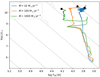 |
Fig. 1. HR diagram of the models at Z = 3 Z⊙. The black circles indicate the point of GR instability. |
where κ ≃ 0.2(1 + X) cm2 g−1 is the opacity, dominated by electron scattering. The effective temperature shows strong oscillations due to the low resolution in the outter layers, but the star remains a ‘red supergiant protostar’ (Hosokawa et al. 2012, 2013; Haemmerlé et al. 2018a) all along the evolution, following the Hayashi limit up to luminosities of 1010 − 1011 L⊙.
The internal structure of some of the models are shown in Figure 2. Once the star is supermassive (M ≳ 104 − 105 M⊙), it is made of a convective core, where convection is driven by H-burning, a ‘radiative’ zone (full of small transient convective zones) and a convective envelope due to the low temperatures and high opacities on the Hayashi limit. The convective envelope is thinner for higher accretion rates. Although the photospheric radius keeps growing, all the Lagrangian layers are contracting, except in the convective core, where the heat liberated by H-burning causes the gas to expand. We see again the oscillations of the surface already visible in Figure 1. Each expansion of the photospheric radius results in the deepening of the convective envelope. Once it enters the radiative region, the gas accreted during such events retains a ‘memory’ of it, displaying a higher density of transient convective zones compared to the other layers (see e.g. the layers 104 M⊙ < Mr < 105 M⊙ in the lower left panel of Figure 2). Inversely, the layers accreted during a contraction show a lower density of transient convective zones (see e.g. the layers 104 M⊙ < Mr < 105 M⊙ in the upper right panel of Figure 2).
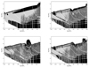 |
Fig. 2. Internal structures of the models (upper left panel: Z = 3 Z⊙ and Ṁ = 10 M⊙ yr−1; upper right panel: Z = 3 Z⊙ and Ṁ = 100 M⊙ yr−1; lower left panel: Z = 3 Z⊙ and Ṁ = 1000 M⊙ yr−1; lower right panel: Z = Z⊙ and Ṁ = 100 M⊙ yr−1), as a function of the stellar mass M. The convective zones are shown in black and the radiative zones in grey. The white curves are iso-masses (Lagrangian layers). |
The central temperatures of the models are shown in Figure 3 as a function of the stellar mass. After an initial increase during the pre-main sequence contraction, the central temperatures stabilise to ∼7 × 10⁷ K due to the thermostatic effect of H-burning.
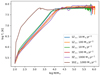 |
Fig. 3. Central temperatures as a function of the stellar mass. |
The entropy profiles of the models at Z = 3 Z⊙ are shown in Figure 4. On each profile, we can distinguish the convective core which is nearly isentropic, the radiative zone where entropy grows outwards, and the thin convective envelope where entropy decreases outwards because of the non-adiabaticity of convection in the low density outter layers. We can see that in the convective core, the entropy is growing due to the heat liberated by H-burning. In the radiative zone, for accretion rates Ṁ > 10 M⊙ yr−1, the successive profiles superimpose to each other, which shows that the evolution is adiabatic in this region of the star: the entropy losses are negligible in the short evolutionary timescale for such rapid accretion. In this case, the entropy profiles adjust on hylotropic profiles s ∝ Mr1/2 (Begelman 2010; Haemmerlé et al. 2019; Haemmerlé 2020). Departures from the hylotropic profiles are visible, which reflects the oscillations of the surface described above: due to the absence of entropy losses, each Lagrangian layer retains the memory of the accretion event. In particular, for the biggest expansion visible in the lower left panel of Figure 2, at a mass ∼30 000 M⊙, we find a plateau in the entropy profiles of the right panel of Figure 4 around the Lagrangian layers Mr ∼ 30 000 M⊙. It is only for accretion rates of Ṁ ≤ 10 M⊙ yr−1 that the evolutionary timescale is long enough for the losses of entropy due to radiative transfer to be visible in the radiative zone.
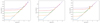 |
Fig. 4. Entropy profiles of the models at Z = 3 Z⊙ (left panel: Ṁ = 10 M⊙ yr−1; central panel: Ṁ = 100 M⊙ yr−1; right panel: Ṁ = 1000 M⊙ yr−1) as a function of the Lagrangian coordinate, at different masses. |
The final masses at GR instability, obtained with Equation (19), are shown for all the models in Table 1 and Figure 5. All the final masses range in the interval 0.6 − 1.2 × 10⁶ M⊙, with a very weak dependence on the metallicity. For accretion rates Ṁ ≲ 100 M⊙ yr−1, the final mass increases as the accretion rate increases. However, for Ṁ ≳ 100 M⊙ yr−1, the final mass is a decreasing function of the accretion rate.
Stellar mass (in 106 M⊙) at the onset of GR instability for indicated metallicities and accretion rates.
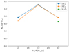 |
Fig. 5. Final mass at GR instability as a function of the accretion rate for the indicated metallicities. |
4. Discussion
4.1. Evolutionary tracks on the HR diagram
The evolutionary tracks of all the models remain in the red on the HR diagram, showing no sign of contraction towards the blue until the GR instability, at luminosities of 1010 − 1011 L⊙. This stands in contrast to the zero-metallicity case, where the tracks start to move to the blue at these luminosities (Hosokawa et al. 2013; Haemmerlé et al. 2018a; Nandal et al. 2024). We interpret this difference as the effect of the larger number density of free electrons for higher metallicity, so that the photosphere is locked on the Hayashi limit towards lower gas densities (Haemmerlé et al. 2019). This fact is key for the problem of the ionising feedback, particularly in the case where other effects postpone the GR instability (rotation, dark matter; Haemmerlé 2021b, 2024). Indeed, in cases where the star moves to the blue for masses ≳105 M⊙, the strong ionising feedback could prevent further accretion (Hosokawa et al. 2011, 2016), limiting the mass to ∼105 M⊙. Here, we see that for metallicities ≥Z⊙, the ionising feedback is expected to remain weak up to masses of at least ∼106 M⊙.
4.2. Internal structures
As shown in Haemmerlé et al. (2019) and Haemmerlé (2020) for lower metallicities, when accretion proceeds at rates ≳10 M⊙ yr−1, the structure of the star is well approximated by hylotropes (Begelman 2010), made of an isentropic core and a radiative envelope where entropy grows outwards, giving, for instance, s ∝ Mr1/2. At these rates, the evolutionary timescale, set by accretion (t ∼ M/Ṁ), is shorter than the Kelvin-Helmholtz (KH) timescale, which prevents any loss of entropy by radiative transfer. The Lagrangian layers of the radiative zone are nevertheless contracting (Figure 2). However this is not a KH contraction, but an adiabatic compression driven by accretion: the weight of the accreted gas induces an increase in the pressure in the whole star and, thus, in the density. As a consequence, the evolution is driven by accretion, all the other processes being too slow to produce any effect. It implies that the structure of the star is essentially given by the stellar mass, independently of the accretion rate. On the other hand, another consequence of the adiabaticity of the evolution is that the successive entropy profiles match each other in the radiative zone: each Lagrangian layer keeps the entropy it advected at accretion. It follows that the oscillations of the surface visible in Figures 1 and 2 have an impact on the whole stellar structure, particularly on the size of the convective core.
The evolutionary tracks on the Mcore − M diagram are shown in Figure 6 for the models at Z = 3 Z⊙. Once the star is supermassive and H-burning has started, the convective core represents typically 10% of the total stellar mass. For a given mass, the model at Ṁ = 10 M⊙ yr−1 has a more massive core than the models with higher accretion rates. This is because of the longer evolutionary timescale in this model, which allows for entropy losses. This gives the layers the time to contract via a KH contraction and join the core, which becomes more massive for a given total mass. On the other hand, for the models at 100−1000 M⊙ yr−1, this effect disappears due to the short evolutionary timescales, so that the Mcore − M relation is nearly unique. Actually, we can see that, for a given mass, this is the model with the shorter timescale that has the more massive core. In this regime of extreme accretion, the evolution of the core is impacted by the advection of the intermediate convective zones, which reflect the oscillations at the stellar surface, as described above. In particular, we can see that the oscillations of the surface at M ∼ 30 000 M⊙ in the model at Ṁ = 1000 M⊙ yr−1 (Figure 2) translate into oscillations in the Mcore − M relation when the layers accreted during the oscillations join the convective core; namely, when Mcore ∼ 30 000 M⊙. At this point, the convective core is growing rapidly due to the advection of a series of isentropic layers, which explains why this model has a larger core than the model at Ṁ = 100 M⊙ yr−1 for a given mass.
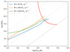 |
Fig. 6. Mcore − M diagram of the models at Z = 3 Z⊙, for the indicated accretion rates. The red line is the hylotropic stability limit with μ = 0.64 and Tc = 7 × 10⁷ K. The grey diagonals indicate constant fractions Mcore/M = 1%−10%−100%. |
Finally, we notice that another reason why the ‘radiative’ zone is prone to transient convective instabilities is that the adiabatic and radiative gradients are both very close to 1/4 in the Eddington limit, as per
 (21)
(21)
 (22)
(22)
 (23)
(23)
where we used the equations of radiative transfer and of hydrostatic equilibrium. We notice the absence of a 𝒪(β) term in the adiabatic gradient.
4.3. Final masses
All the models reached the GR instability during H-burning, so that there is no dark collapse in the sense proposed by Nandal et al. (2024). Indeed, H-burning starts earlier with high metallicity compared to the primordial case because the CNO elements are already present in the initial composition, so we do not need to wait for the 3-α reactions to produce it. As a consequence, H-burning starts at a lower stellar mass, when the star is still GR-stable. Moreover, for the same reason, the central temperature remains lower with high metallicity compared to the primordial case (see Figure 3), which favours GR stability.
All the final masses are ∼106 M⊙, with a weak dependence on the accretion rate and on the metallicity. In particular, the increase in the accretion rate from 100 to 1000 M⊙ yr−1 does not translate into an increase of the final mass as for lower rates. This fact was already noted by Nagele & Umeda (2024) for lower metallicities, but left without explanation. Here, we propose an explanation: because of the adiabaticity of the evolution in this extreme accretion regime, the stellar structure is determined by the mass only and, thus, nearly independently of the accretion rate, as explained in the previous section. Therefore, we can expect a unique final mass for rates of ≳100 M⊙ yr−1. Only the differences in the oscillations of the stellar surface, retained in memory by the gas when it joins the convective core, impact the core’s mass. It leads to a larger core (for given mass) for the model at Ṁ = 1000 M⊙ yr−1, compared to the one at Ṁ = 100 M⊙ yr−1 (Figure 6). As a consequence, the GR instability is reached at a lower mass for the model at Ṁ = 1000 M⊙ yr−1 than for the one at Ṁ = 100 M⊙ yr−1.
Figure 6 compares the final mass of the models at Z = 3 Z⊙, with the hylotropic stability limit (Haemmerlé 2020). The hylotropic limit is computed for a mean molecular weight of μ = 0.64 and a central temperature of Tc = 7 × 10⁷ K, typical values for Z = 3 Z⊙ SMSs in the beginning of H-burning. We see that the models slightly exceed this analytic limit, but only by a maximum of 0.2 dex in M. Thus, the hylotropic limit represents a good approximation for the models. It illustrates that the larger is the convective core the smaller is the final mass, explaining why the model at Ṁ = 1000 M⊙ yr−1 has a lower final mass than that at Ṁ = 100 M⊙ yr−1.
5. Conclusion
In the present work, we study, for the first time, the properties of SMSs at Z > Z⊙, focussing on the conditions met in galaxy merger driven direct collapse (Z = 1 − 10 Z⊙, Ṁ = 10−1000 M⊙ yr−1). We neglected rotation, which will be the topic of the next paper of the series.
We found that at these accretion rates and metallicities, SMSs evolve as red supergiant protostars until the GR instability (Figure 1). The internal structure is made of an isentropic convective core that contains ∼10% of the total stellar mass, along with a ‘radiative’ region full of small transient convective zones, where entropy grows outwards following a hylotropic law, and a thin convective envelope with an entropy decreasing outwards due to the non-adiabaticity of convection in the low-density regions (Figures 2–4). For accretion rates of > 10 M⊙ yr−1, the evolution in the radiative region is adiabatic (Figure 4): the Lagrangian layers are contracting; however this is not a KH contraction, but an adiabatic compression that is driven by accretion. As a consequence, in this extreme accretion regime, the stellar structure is set essentially by the stellar mass, independently of the accretion rate. This results in a nearly unique final mass ∼106 M⊙ for all the models (Figure 5). Moreover, all the models reach GR instability during H-burning.
References
- Appenzeller, I., & Fricke, K. 1972a, A&A, 18, 10 [NASA ADS] [Google Scholar]
- Appenzeller, I., & Fricke, K. 1972b, A&A, 21, 285 [NASA ADS] [Google Scholar]
- Asplund, M., Grevesse, N., & Sauval, A. J. 2005, ASP Conf. Ser., 336, 25 [Google Scholar]
- Bañados, E., Venemans, B. P., Mazzucchelli, C., et al. 2018, Nature, 553, 473 [Google Scholar]
- Begelman, M. C. 2010, MNRAS, 402, 673 [NASA ADS] [CrossRef] [Google Scholar]
- Bogdán, Á., Goulding, A. D., Natarajan, P., et al. 2024, Nat. Astron., 8, 126 [Google Scholar]
- Bromm, V., & Loeb, A. 2003, ApJ, 596, 34 [Google Scholar]
- Bromm, V., Coppi, P. S., & Larson, R. B. 2002, ApJ, 564, 23 [Google Scholar]
- Chandrasekhar, S. 1964, ApJ, 140, 417 [Google Scholar]
- Chon, S., Hosokawa, T., & Yoshida, N. 2018, MNRAS, 475, 4104 [CrossRef] [Google Scholar]
- Dijkstra, M., Haiman, Z., Mesinger, A., & Wyithe, J. S. B. 2008, MNRAS, 391, 1961 [NASA ADS] [CrossRef] [Google Scholar]
- Eggenberger, P., Meynet, G., Maeder, A., et al. 2008, Ap&SS, 316, 43 [Google Scholar]
- Fuller, G. M., Woosley, S. E., & Weaver, T. A. 1986, ApJ, 307, 675 [Google Scholar]
- Haemmerlé, L. 2020, A&A, 644, A154 [NASA ADS] [CrossRef] [EDP Sciences] [Google Scholar]
- Haemmerlé, L. 2021a, A&A, 647, A83 [NASA ADS] [CrossRef] [EDP Sciences] [Google Scholar]
- Haemmerlé, L. 2021b, A&A, 650, A204 [NASA ADS] [CrossRef] [EDP Sciences] [Google Scholar]
- Haemmerlé, L. 2024, A&A, 689, A202 [NASA ADS] [CrossRef] [EDP Sciences] [Google Scholar]
- Haemmerlé, L., Eggenberger, P., Meynet, G., Maeder, A., & Charbonnel, C. 2016, A&A, 585, A65 [NASA ADS] [CrossRef] [EDP Sciences] [Google Scholar]
- Haemmerlé, L., Woods, T. E., Klessen, R. S., Heger, A., & Whalen, D. J. 2018a, MNRAS, 474, 2757 [Google Scholar]
- Haemmerlé, L., Woods, T. E., Klessen, R. S., Heger, A., & Whalen, D. J. 2018b, ApJ, 853, L3 [Google Scholar]
- Haemmerlé, L., Meynet, G., Mayer, L., et al. 2019, A&A, 632, L2 [NASA ADS] [CrossRef] [EDP Sciences] [Google Scholar]
- Haemmerlé, L., Mayer, L., Klessen, R. S., et al. 2020, Space Sci. Rev., 216, 48 [Google Scholar]
- Haemmerlé, L., Klessen, R. S., Mayer, L., & Zwick, L. 2021, A&A, 652, L7 [NASA ADS] [CrossRef] [EDP Sciences] [Google Scholar]
- Haiman, Z., Rees, M. J., & Loeb, A. 1997, ApJ, 476, 458 [NASA ADS] [CrossRef] [Google Scholar]
- Herrington, N. P., Whalen, D. J., & Woods, T. E. 2023, MNRAS, 521, 463 [CrossRef] [Google Scholar]
- Hosokawa, T., Omukai, K., Yoshida, N., & Yorke, H. W. 2011, Science, 334, 1250 [CrossRef] [Google Scholar]
- Hosokawa, T., Omukai, K., & Yorke, H. W. 2012, ApJ, 756, 93 [Google Scholar]
- Hosokawa, T., Yorke, H. W., Inayoshi, K., Omukai, K., & Yoshida, N. 2013, ApJ, 778, 178 [Google Scholar]
- Hosokawa, T., Hirano, S., Kuiper, R., et al. 2016, ApJ, 824, 119 [NASA ADS] [CrossRef] [Google Scholar]
- Klessen, R. S., & Glover, S. C. O. 2023, ARA&A, 61, 65 [NASA ADS] [CrossRef] [Google Scholar]
- Kokorev, V., Fujimoto, S., Labbe, I., et al. 2023, ApJ, 957, L7 [NASA ADS] [CrossRef] [Google Scholar]
- Kovács, O. E., Bogdán, Á., Natarajan, P., et al. 2024, ApJ, 965, L21 [CrossRef] [Google Scholar]
- Larson, R. L., Finkelstein, S. L., Kocevski, D. D., et al. 2023, ApJ, 953, L29 [NASA ADS] [CrossRef] [Google Scholar]
- Latif, M. A., Schleicher, D. R. G., Schmidt, W., & Niemeyer, J. C. 2013, MNRAS, 436, 2989 [Google Scholar]
- Maiolino, R., Scholtz, J., Witstok, J., et al. 2024, Nature, 627, 59 [NASA ADS] [CrossRef] [Google Scholar]
- Mayer, L., Kazantzidis, S., Escala, A., & Callegari, S. 2010, Nature, 466, 1082 [Google Scholar]
- Mayer, L., Fiacconi, D., Bonoli, S., et al. 2015, ApJ, 810, 51 [Google Scholar]
- Mayer, L., Capelo, P. R., Zwick, L., & Di Matteo, T. 2024, ApJ, 961, 76 [NASA ADS] [CrossRef] [Google Scholar]
- Montero, P. J., Janka, H.-T., & Müller, E. 2012, ApJ, 749, 37 [Google Scholar]
- Nagele, C., & Umeda, H. 2024, Phys. Rev. D, 110, L061301 [Google Scholar]
- Nagele, C., Umeda, H., Takahashi, K., Yoshida, T., & Sumiyoshi, K. 2022, MNRAS, 517, 1584 [NASA ADS] [CrossRef] [Google Scholar]
- Nandal, D., Regan, J. A., Woods, T. E., et al. 2023, A&A, 677, A155 [NASA ADS] [CrossRef] [EDP Sciences] [Google Scholar]
- Nandal, D., Zwick, L., Whalen, D. J., et al. 2024, A&A, 689, A351 [NASA ADS] [CrossRef] [EDP Sciences] [Google Scholar]
- Omukai, K. 2001, ApJ, 546, 635 [NASA ADS] [CrossRef] [Google Scholar]
- Regan, J. A., Visbal, E., Wise, J. H., et al. 2017, Nat. Astron., 1, 0075 [Google Scholar]
- Saio, H., Nandal, D., Ekström, S., & Meynet, G. 2024, A&A, 689, A169 [NASA ADS] [CrossRef] [EDP Sciences] [Google Scholar]
- Schauer, A. T. P., Regan, J., Glover, S. C. O., & Klessen, R. S. 2017, MNRAS, 471, 4878 [NASA ADS] [CrossRef] [Google Scholar]
- Umeda, H., Hosokawa, T., Omukai, K., & Yoshida, N. 2016, ApJ, 830, L34 [Google Scholar]
- Wang, F., Yang, J., Fan, X., et al. 2018, ApJ, 869, L9 [NASA ADS] [CrossRef] [Google Scholar]
- Wang, F., Yang, J., Fan, X., et al. 2021, ApJ, 907, L1 [Google Scholar]
- Woods, T. E., Heger, A., Whalen, D. J., Haemmerlé, L., & Klessen, R. S. 2017, ApJ, 842, L6 [Google Scholar]
- Woods, T. E., Agarwal, B., Bromm, V., et al. 2019, PASA, 36, e027 [Google Scholar]
- Woods, T. E., Patrick, S., Elford, J. S., Whalen, D. J., & Heger, A. 2021, ApJ, 915, 110 [NASA ADS] [CrossRef] [Google Scholar]
- Woods, T. E., Patrick, S., Whalen, D. J., & Heger, A. 2024, ApJ, 960, 59 [NASA ADS] [CrossRef] [Google Scholar]
- Wu, X.-B., Wang, F., Fan, X., et al. 2015, Nature, 518, 512 [Google Scholar]
- Yang, J., Wang, F., Fan, X., et al. 2020, ApJ, 897, L14 [Google Scholar]
- Zwick, L., Mayer, L., Haemmerlé, L., & Klessen, R. S. 2023, MNRAS, 518, 2076 [Google Scholar]
All Tables
Stellar mass (in 106 M⊙) at the onset of GR instability for indicated metallicities and accretion rates.
All Figures
|
Fig. 1. HR diagram of the models at Z = 3 Z⊙. The black circles indicate the point of GR instability. |
| In the text | |
|
Fig. 2. Internal structures of the models (upper left panel: Z = 3 Z⊙ and Ṁ = 10 M⊙ yr−1; upper right panel: Z = 3 Z⊙ and Ṁ = 100 M⊙ yr−1; lower left panel: Z = 3 Z⊙ and Ṁ = 1000 M⊙ yr−1; lower right panel: Z = Z⊙ and Ṁ = 100 M⊙ yr−1), as a function of the stellar mass M. The convective zones are shown in black and the radiative zones in grey. The white curves are iso-masses (Lagrangian layers). |
| In the text | |
|
Fig. 3. Central temperatures as a function of the stellar mass. |
| In the text | |
|
Fig. 4. Entropy profiles of the models at Z = 3 Z⊙ (left panel: Ṁ = 10 M⊙ yr−1; central panel: Ṁ = 100 M⊙ yr−1; right panel: Ṁ = 1000 M⊙ yr−1) as a function of the Lagrangian coordinate, at different masses. |
| In the text | |
|
Fig. 5. Final mass at GR instability as a function of the accretion rate for the indicated metallicities. |
| In the text | |
|
Fig. 6. Mcore − M diagram of the models at Z = 3 Z⊙, for the indicated accretion rates. The red line is the hylotropic stability limit with μ = 0.64 and Tc = 7 × 10⁷ K. The grey diagonals indicate constant fractions Mcore/M = 1%−10%−100%. |
| In the text | |
Current usage metrics show cumulative count of Article Views (full-text article views including HTML views, PDF and ePub downloads, according to the available data) and Abstracts Views on Vision4Press platform.
Data correspond to usage on the plateform after 2015. The current usage metrics is available 48-96 hours after online publication and is updated daily on week days.
Initial download of the metrics may take a while.