| Issue |
A&A
Volume 700, August 2025
|
|
|---|---|---|
| Article Number | A63 | |
| Number of page(s) | 7 | |
| Section | Extragalactic astronomy | |
| DOI | https://doi.org/10.1051/0004-6361/202554375 | |
| Published online | 06 August 2025 | |
Spectral indices in active galactic nuclei as seen by Apertif and LOFAR
1
ASTRON, The Netherlands Institute for Radio Astronomy, Oude Hoogeveensedijk 4, 7991 PD, Dwingeloo, The Netherlands
2
Kapteyn Astronomical Institute, P.O. Box 800 9700 AV, Groningen, The Netherlands
3
School of Physical Sciences and Nanotechnology, Yachay Tech University, Hacienda San José S/N, 100119 Urcuquí, Ecuador
⋆ Corresponding author: This email address is being protected from spambots. You need JavaScript enabled to view it.
Received:
4
March
2025
Accepted:
27
May
2025
Abstract
We present two new radio continuum images obtained with Apertif at 1.4 GHz. The images, produced with a direction-dependent calibration pipeline, cover 136 square degrees of the Lockman Hole and 24 square degrees of the ELAIS-N fields, with an average resolution of 17 × 12″ and a residual noise of 33 μJy beam−1. With the improved depth of the images, we find a total of 63 692 radio sources, many of which are detected for the first time at this frequency. With the addition of the previously published Apertif catalog for the Boötes field, we cross-matched it with the LOFAR deep-fields value-added catalogs at 150 MHz, resulting in a homogeneous sample of 10 196 common sources with spectral index estimates – one of the largest to date. We analyze and discuss the correlations between the spectral index, redshift, linear source size, and radio luminosity, taking into account biases of flux-density-limited surveys. Our results suggest that the observed correlation between spectral index and redshift of active galactic nuclei can be attributed to the Malmquist bias, reflecting an intrinsic relation between radio luminosity and the spectral index. We also find a correlation between the spectral index and linear source size, with more compact sources having steeper spectra.
Key words: catalogs / surveys / galaxies: active / radio continuum: galaxies / radio continuum: general
© The Authors 2025
 Open Access article, published by EDP Sciences, under the terms of the Creative Commons Attribution License (https://creativecommons.org/licenses/by/4.0), which permits unrestricted use, distribution, and reproduction in any medium, provided the original work is properly cited.
This article is published in open access under the Subscribe to Open model. This email address is being protected from spambots. You need JavaScript enabled to view it. to support open access publication.
1. Introduction
The shape of the radio spectral energy distribution of active galactic nuclei (AGNs) carries information about the emission mechanisms, the physical properties of the sources, and their evolutionary stage (Morganti 2017; Hardcastle & Croston 2020, and references therein). The radio spectrum from synchrotron emission is often well-described by a power law, characterized by the spectral index α, defined as Sν ∝ να, where Sν is the flux density at frequency ν. Deviations from this power law are clear signatures of, for example, energy losses or absorption processes that can be observed at high and low frequencies, respectively. These features move in frequency not only with the age, but also with the redshift of the source, as nicely illustrated by the sketch in Fig. 2 of Ker et al. (2012).
Spectral indices of radio sources typically range from −1.5 to 0.5, with the majority falling between −0.8 and −0.7 (Condon 1992; Mahony et al. 2016). Steep spectrum sources (α < −0.7) are often associated with extended radio lobes, while flat spectrum sources (−0.5 < α < 0) are generally compact and may indicate self-absorbed synchrotron emission (e.g., Kellermann 1966). Inverted spectrum sources (α > 0) are less common and may be associated with young or highly compact absorbed objects (O’Dea 1998; O’Dea & Saikia 2021).
A relation between spectral index and redshift has already been noted in the early studies of radio sources (Blumenthal & Miley 1979), with higher redshift sources tending to have steeper spectra. This relation played a key role in discovering the first high redshift galaxies, which, for this reason, were all radio galaxies (e.g., Roettgering et al. 1994; Miley & De Breuck 2008).
As summarized by Miley & De Breuck (2008), the relation that more distant sources have steeper spectra was originally interpreted as resulting from a combination of a concave radio spectrum (caused by synchrotron and inverse Compton (IC) energy losses at high frequencies) and the k-correction, in which the steeper part of the radio spectrum enters the typical observed frequency range for high-z sources. However, Klamer et al. (2006) showed a lack of strong curvature in the spectra of their sources, in direct contradiction to this explanation.
Alternative explanations for this relation have also been proposed. These include: enhanced spectral aging due to increased IC losses against the cosmic microwave background (CMB) radiation at high redshifts (Klamer et al. 2006; Morabito & Harwood 2018, and references therein); an intrinsic correlation between low-frequency spectral index and radio luminosity, with higher luminosities corresponding to higher jet powers, which produce stronger magnetic fields, resulting in more rapid electron cooling times (Chambers et al. 1990; Blundell et al. 1999); and higher ambient density at high redshifts, which can cause steeper electron energy spectra (Athreya & Kapahi 1998; Klamer et al. 2006).
The study of the spectral properties for large samples of radio sources is currently facilitated by large-scale radio surveys across different frequencies (see Norris 2017, for an overview of the surveys). The LOFAR Two-meter Sky Survey (LoTSS; Shimwell et al. 2017, 2022), with unprecedented sensitivity and resolution, has extended the detailed study of the spectral index to low frequencies. Furthermore, the availability of value-added catalogs for the LOFAR sources, which crucially include redshifts, makes them particularly well suited for tracing the evolution of their properties. At present, a bottleneck for probing spectral indices is the availability of a survey at GHz frequencies that is deep enough to match the sensitivity of LOFAR. Shallow 1.4 GHz surveys can bias samples towards flatter spectrum sources at higher redshifts (Ker et al. 2012), while deep surveys usually focus on small sky areas lacking sources for statistical studies. This has placed the onus on higher frequency surveys to match the sensitivity and sky coverage of LOFAR. One example is the 1.4 GHz continuum survey with Apertif, presented and released partially in this paper.
A recent study by Kutkin et al. (2023, K23) probed spectral indices within the 26.5 square degree region of the Boötes constellation using the LOFAR HBA at 150 MHz and the LOFAR LBA at 50 MHz as well as Apertif images at 1.4 GHz. They found that the redshift dependence is different for the low- (50–150 MHz) and high-frequency (150–1400 MHz) spectral index. The first one drops steeply at lower redshifts and decreases more slowly at higher redshifts, while the second one only shows a weak linear trend throughout the entire redshift range. This can be explained by a population of peaked spectrum sources appearing at lower frequencies. In another recent work, Pinjarkar et al. (2025), the authors claim that the correlation between spectral index and redshift is driven by the dependence of the former on luminosity and by a strong redshift-luminosity correlation occurring in flux density-limited samples, (also known as, the Malmquist bias). This naturally motivates further work with larger sample sizes, especially at high redshifts, and a more detailed investigation of any correlation of spectral index with other parameters (e.g., luminosity and linear source size).
In this work we take this next step by examining spectral indices between 1.4 GHz and 150 MHz over almost 200 square degrees. The paper is organized as follows: In Sect. 2 we present the new 1.4 GHz images and catalogs obtained with Apertif. In Sect. 3 we describe the combination of LOFAR and Apertif data. The analysis of spectral index and other source parameters is presented in Sect. 4. Our results and conclusions are discussed in Sect. 5.
Throughout this paper we assume a flat ΛCDM cosmology model with H0 = 70 km/(s Mpc), ΩM = 0.3, implemented by the Astropy Python library (Astropy Collaboration 2018). We use a positively defined spectral index, α = dlnS/dlnν.
2. Apertif images and catalogs
Apertif is a phased-array feed system that was mounted on the Westerbork synthesis radio telescope (WSRT), providing a field-of-view of 10 square degrees (van Cappellen et al. 2022). Apertif enabled large-scale radio continuum, polarization, and spectral line surveys, which were supported by automated processing with a custom pipeline (Adams et al. 2022; Adebahr et al. 2022).
In Kutkin et al. (2022, K22) the radio continuum images and catalog from the first data release are described. More recently, the pipeline for producing radio continuum images has been improved with the addition of direction-dependent calibration, as described in K23, where the improved images for the Boötes region were presented. Here, we expand on this by presenting mosaic images of two additional well-known regions of the northern sky: ELAIS-N and Lockman Hole, produced with the new pipeline.
The reduction and imaging of the data were done following the same procedure used for the Boötes field. The individual compound beam images produced with the improved pipeline were corrected for an astrometric offset and primary beam shape, brought to the same resolution, re-projected to a common sky grid, and linearly mosaicked into a larger image (see K22 and K23 for details). Because of the overlap of the individual Apertif images, the mosaicking leads to an increase in sensitivity. The mosaic images of the ELAIS-N and Lockman Hole fields along with the corresponding residual noise maps are shown in Fig. 1. The images and the catalogs are published on the ASTRON VO server at https://vo.astron.nl. An example of the catalog records for the ELAIS-N field is shown in Table 1.
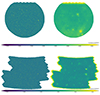 |
Fig. 1. Mosaic images of the ELAIS-N (top) and Lockman Hole (bottom) fields along with the noise RMS maps. |
Apertif source list.
The corresponding source catalogs were extracted for these two fields using the PyBDSF source finder (Mohan & Rafferty 2015), in the same way as for the Boötes field by K23. The flux density and coordinate uncertainties were corrected for the systematic calibration errors. The false detection rate, below 2%, was estimated as the number of sources detected in the inverted image over the number of sources in the original image. The completeness of all three catalogs was estimated to be 0.3 mJy by comparing the differential source counts to Matthews et al. (2021). This is illustrated in Fig. 2 (see also K22 and K23 for details). We note that the completeness and reliability estimates may have local variations following the changes in local noise RMS (see Fig. 1).
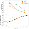 |
Fig. 2. False-detection fraction and differential source counts in the Apertif catalog. |
For further analysis we combined the catalogs of all three fields, as summarized in Table 2. We note that individual Apertif images were obtained with a slightly different central frequency and bandwidth (1350 MHz/150 MHz before January 2021 and 1375 MHz/250 MHz after). For the new frequency setup, we derived the corresponding primary beam models, which were accounted for during the mosaicking procedure. In this work, we did not trace the primary beam shape variations at higher cadence, which may have contributed to some systematic errors. However, since the mosaics are produced using more than one compound beam image taken at different epochs, we expect these errors to average out and be well below the general calibration errors. For further analysis we calculated a median offset between the Apertif and NVSS total flux density and corrected the former by this factor, which is within a few percent for all three catalogs. Accordingly, we adopted the central frequency of 1400 MHz.
Apertif data.
3. Combination with LOFAR
The same deep fields were observed by LOFAR, and an extensive data analysis was performed on these observations (Tasse et al. 2021; Sabater et al. 2021). As demonstrated by K22 and K23, the combination of the Apertif and LOFAR surveys (at 1400 MHz and 150 MHz) provides great synergy due to their common sky coverage, similar angular resolution, and high sensitivity. This combination allows us to probe spectral indexes of the sources at flux densities and redshifts unreachable before.
We used the LOFAR value-added deep field catalogs available through the official LOFAR website1 (Duncan et al. 2019; Kondapally et al. 2021). For the redshift estimate, we used the column labeled “Z_BEST”, which provides the best available redshift, either spectroscopic or photometric.
We cross-matched the source coordinates between the Apertif and LOFAR samples using a 5″ radius and obtained a sample of 10 196 sources, 96% of which have redshift measurements. The spectral indices were estimated as:  , where
  and
and  denote the Apertif and LOFAR integrated flux density. The spectral index error estimate is propagated from flux density uncertainties. These data are summarized in Table 3 for all 10 196 common sources.
Common Apertif and LOFAR sources.
4. Analysis and results
4.1. Spectral index and total flux density
As mentioned above, the Apertif catalog is complete down to the 0.3 mJy level. Below this level, a source may be missing from the Apertif catalog while still being detected by LOFAR, unless it has a flat spectrum. This results in a bias of the average spectral index estimate for sources with low flux density, as shown in the left panel of Fig. 3, where the distribution of spectral indices as a function of LOFAR integrated flux density is plotted for the common sources. It is clear that, below a few millijanskys, the spectral index distribution is affected by incompleteness due to missing steep spectrum sources in the Apertif survey. To exclude this bias, we limited our analysis to the threshold  mJy, where the spectral index distribution becomes symmetric and its median value does not change significantly with flux density (see left plot of Fig. 3). As a result, we obtained a sample of 2437 sources, out of which 2273 have redshift estimates, further referred to as the main sample. Such a selection also implies that a great majority of the considered sources are radio-loud AGNs, which dominate the population at LOFAR flux densities above 3 mJy (see Fig. 10 and discussion by Best et al. 2023).
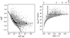 |
Fig. 3. Left: Spectral index against the LOFAR integrated flux density for all common Apertif and LOFAR sources. The markers show the median spectral index in a given flux density interval. The solid line indicates a lower limit calculated for the Apertif completeness level of 0.3 mJy (Sect. 4.1). Right: Luminosity against redshift for the main sample. The solid lines indicate a Malmquist bias-free region (Sect. 4.2). |
4.2. Spectral index and luminosity
We calculated the radio luminosity density in the source frame as: Lν = 4πDL2Sintν(1 + z)−(1 + α), where DL is the luminosity distance and Sνint the observed total flux density (e.g., Klamer et al. 2006).
In the right panel of Fig. 3, the radio luminosity is plotted against redshift for the main sample. Unsurprisingly, detectable source luminosities depend strongly on the redshift, resulting in a Malmquist bias when considering source properties at different redshifts. To account for this bias, we subsequently considered a subsample of sources with luminosities above 5 ⋅ 1025 W/Hz and redshifts above 0.4, shown with solid lines in the right panel of Fig. 3. This includes 543 sources and shows no correlation between luminosity and redshift.
In the top left panel of Fig. 4, the distribution of spectral index against luminosity is shown for the main sample. To trace the correlation, we binned the X-axis into bins containing equal numbers of sources; the edges of these bins are indicated by vertical dashed lines. Within each bin, we calculated the median spectral index and average X-coordinate. These measurements are plotted with square markers, along with their 95% confidence intervals estimated using bootstrap. We then used Markov chain Monte Carlo (MCMC) simulations (Foreman-Mackey et al. 2013) with a linear model, y = ax + b, to determine the correlation coefficient, a, shown in the top right corner. The solid gray lines show random samples drawn from an MCMC posterior distribution.
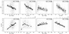 |
Fig. 4. Top row: Spectral index vs. luminosity and linear source size for the main sample (Columns 1–2) and the Malmquist-bias-free subsample (Columns 3–4). Bottom row: Linear source size against luminosity and redshift for the same samples (see Sects. 4.2 and 4.3 for details). |
There is a weak correlation, with more luminous sources showing steeper spectra following α ∝ L−0.03. This correlation holds, with larger uncertainties, for the Malmquist-bias-free subsample, as shown on the third panel of Fig. 4.
4.3. Spectral index and source size
Linear source size can be estimated as D150 = θ150DA, where θ150 is the LOFAR deconvolved source size (PyBDSF: DC_Maj) and DA is the angular diameter distance. To trace the correlation between the linear size and other parameters, we considered only sources with θ150 > 0. As shown in the second panel of Fig. 4, there is a correlation, with larger sources having steeper spectra following α ∝ D−0.1. This trend holds, if we consider the Malmquist-bias-free subsample (see Sect. 4.2 and the fourth panel of Fig. 4).
In the second row of Fig. 4, the linear source size is plotted against luminosity and redshift for the main sample and the Malmquist-bias-free subsample. While there is an expected trend for more luminous sources to have larger sizes, the dependence of size on redshift is not monotonic [see also][for discussion]2012MNRAS.420.2644K.
4.4. Spectral index and redshift
The distribution of spectral indices against redshift is presented in Fig. 5. The individual sources are indicated by gray dots. Binning is done in the same way as in Fig. 4. For each interval, we calculated the average redshift and median spectral index, plotted with square markers. The uncertainties were estimated using bootstrap performed within each bin. The two plots present the trend for the main sample and for the Malmquist-bias-free subsample, plotted with the same binning. The slope coefficients and their errors obtained using a linear model and MCMC simulations are illustrated in Fig. 6.
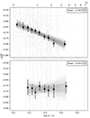 |
Fig. 5. Spectral index against redshift for all sources (top) and the Malmquist-bias-free subsample (bottom). |
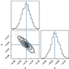 |
Fig. 6. Parameter distributions of the MCMC fit with a linear model, α(z) = a z + b, shown in the top panel of Fig. 5. Vertical and horizontal lines show the maximum a posteriori (MAP) estimate of the parameters. |
The top plot shows a clear correlation with steeper spectra at high redshift. The slope, α ∝ log(1 + z)−0.3 ± 0.1 obtained for the main sample agrees within errors with the results of K23. As mentioned in the introduction, this well-known trend is used to select high-redshift sources based on their steep spectra. However, there is no α-z correlation for the Malmquist-bias-free subsample, as seen in the bottom panel of Fig. 5 (see also Sect. 4.2). This implies that we see steeper spectra at higher redshifts mostly due to the combination of α-L correlation and the Malmquist bias.
5. Discussion and conclusions
We processed Apertif observations and presented two new radio continuum images and catalogs at 1.4 GHz. Due to the higher sensitivity of Apertif compared to previous northern surveys, many radio sources were detected for the first time at these frequencies. The images cover more than 150 square degrees within the well-known fields, ELAIS-N and Lockman Hole, observed at many other facilities at various frequencies. With the addition of the previously published catalog for the Boötes field, we cross-matched Apertif source coordinates with those in LOFAR value-added catalogs to probe spectral indices and other parameters of radio sources. We compiled and studied a new sample of common Apertif and LOFAR sources, complete in terms of spectral index and including enough data for a statistical analysis, which is especially crucial for high redshift sources. We constrained and separately studied a subsample of sources free from Malmquist bias.
The median spectral index of radio sources shows an anticorrelation with luminosity and linear source size: the more powerful and more extended sources tend to have steeper spectra. The observed positive correlation between size and luminosity agrees well with this trend. The observed correlation between spectral index and redshift can be attributed to the Malmquist bias and the intrinsic α-L correlation. This can be explained with a model proposed by Kardashev (1962), where an optically thin part of a radio spectrum experiences a break from α0 to α0 − 0.5 when the radiation loss timescale becomes comparable to the injection timescale. The break frequency is inversely proportional to the jet magnetic field strength, νbreak ∝ B−3, while the total radio luminosity is proportional to B3.5. Therefore, more luminous sources experience spectral break at lower frequencies (see, e.g., Chambers et al. 1990, for details).
Despite removing the Malmquist bias, a significant anticorrelation continues to exist between α-D and D-z. The first correlation can be explained by source aging: older sources that have had enough time to grow to larger sizes have steeper spectra. The second correlation may be related to younger and, hence, smaller sources seen at higher redshifts. At the same time, no correlation of α-z is observed after eliminating the Malmquist bias, implying that another mechanism is responsible for the steepening of radio spectra at higher redshifts, unrelated to α(L, D). This may be more efficient electron cooling through IC losses due to a denser environment at higher redshifts. Thus, we can speculate about two concurring trends eliminating the α-z correlation: IC losses cause the spectra to become steeper, while a population of compact sources with flatter spectra arises at higher redshifts (see Ker et al. 2012; Morabito & Harwood 2018, for more discussion).
Interestingly, Ker et al. (2012), who used combined smaller samples, reported a weak α-z correlation even after removing the Malmquist bias. We confirm a slight, insignificant trend with a negative slope when the sample is constrained to α < −0.5, as done in the work mentioned above. The authors excluded a population of bright sources with flatter spectra that appear at higher redshifts, represented by compact BL Lacertae objects and flat spectrum radio quasars. In this work, we consider a sample to be complete in terms of spectral index, as the distribution of the latter is continuous across all redshift ranges.
The intrinsic scatter in the spectral index distribution and the weak α-z correlation, even within the total biased sample, do not allow for the reliable identification of high-redshift sources based solely on their steep spectra. More robust results can be achieved by involving other parameters, such as linear source size.
Apertif, with its angular resolution, sensitivity, and sky coverage, is an excellent complement to the LOFAR observations, allowing not only statistical studies of radio spectra but also the probing of internal structures within extended sources. We continue processing the observations and releasing new images for the community.
Data availability
Full Tables 1 and 3 are available at at the CDS via https://cdsarc.cds.unistra.fr/viz-bin/cat/J/A+A/700/A63 and at http://vo.astron.nl The mosaic images are also available at the CDS via https://cdsarc.cds.unistra.fr/viz-bin/cat/J/A+A/700/A63 and at http://vo.astron.nl
Acknowledgments
This work makes use of data from the Apertif system installed at the Westerbork Synthesis Radio Telescope owned by ASTRON. ASTRON, the Netherlands Institute for Radio Astronomy, is an institute of the Dutch Science Organisation (De Nederlandse Organisatie voor Wetenschappelijk Onderzoek, NWO). Apertif was partly financed by the NWO Groot projects Apertif (175.010.2005.015) and Apropos (175.010.2009.012). This research made use of Python programming language with its standard and external libraries/packages including numpy (Harris et al. 2020), scipy (Virtanen et al. 2020), scikit-learn (Pedregosa et al. 2011), matplotlib (Hunter 2007), pandas (The Pandas development team 2020) etc. This research made use of Astropy (http://www.astropy.org), a community-developed core Python package for Astronomy (Astropy Collaboration 2013, 2018). The radio_beam and reproject python packages are used for manipulations with restoring beam and reprojecting/mosaicking of the images. This research has made use of “Aladin sky atlas” developed at CDS, Strasbourg Observatory, France (Bonnarel et al. 2000; Boch & Fernique 2014).
References
- Adams, E. A. K., Adebahr, B., de Blok, W. J. G., et al. 2022, A&A, 667, A38 [NASA ADS] [CrossRef] [EDP Sciences] [Google Scholar]
- Adebahr, B., Schulz, R., Dijkema, T. J., et al. 2022, Astron. Comput., 38, 100514 [NASA ADS] [CrossRef] [Google Scholar]
- Astropy Collaboration (Robitaille, T. P., et al.) 2013, A&A, 558, A33 [NASA ADS] [CrossRef] [EDP Sciences] [Google Scholar]
- Astropy Collaboration (Price-Whelan, A. M., et al.) 2018, AJ, 156, 123 [Google Scholar]
- Athreya, R. M., & Kapahi, V. K. 1998, JApA, 19, 63 [Google Scholar]
- Best, P. N., Kondapally, R., Williams, W. L., et al. 2023, MNRAS, 523, 1729 [NASA ADS] [CrossRef] [Google Scholar]
- Blumenthal, G., & Miley, G. 1979, A&A, 80, 13 [NASA ADS] [Google Scholar]
- Blundell, K. M., Rawlings, S., & Willott, C. J. 1999, AJ, 117, 677 [Google Scholar]
- Boch, T., & Fernique, P. 2014, in Astronomical Data Analysis Software and Systems XXIII, eds. N. Manset, & P. Forshay, Astronomical Society of the Pacific Conference Series, 485, 277 [NASA ADS] [Google Scholar]
- Bonnarel, F., Fernique, P., Bienaymé, O., et al. 2000, A&AS, 143, 33 [NASA ADS] [CrossRef] [EDP Sciences] [Google Scholar]
- Chambers, K. C., Miley, G. K., & van Breugel, W. J. M. 1990, ApJ, 363, 21 [NASA ADS] [CrossRef] [Google Scholar]
- Condon, J. J. 1992, ARA&A, 30, 575 [Google Scholar]
- Duncan, K. J., Sabater, J., Röttgering, H. J. A., et al. 2019, A&A, 622, A3 [NASA ADS] [CrossRef] [EDP Sciences] [Google Scholar]
- Foreman-Mackey, D., Hogg, D. W., Lang, D., & Goodman, J. 2013, PASP, 125, 306 [Google Scholar]
- Hardcastle, M. J., & Croston, J. H. 2020, New Astron. Rev., 88, 101539 [Google Scholar]
- Harris, C. R., Millman, K. J., van der Walt, S. J., et al. 2020, Nature, 585, 357 [NASA ADS] [CrossRef] [Google Scholar]
- Hunter, J. D. 2007, Comput. Sci. Eng., 9, 90 [NASA ADS] [CrossRef] [Google Scholar]
- Kardashev, N. S. 1962, Soviet Ast., 6, 317 [Google Scholar]
- Kellermann, K. I. 1966, ApJ, 146, 621 [NASA ADS] [CrossRef] [Google Scholar]
- Ker, L. M., Best, P. N., Rigby, E. E., Röttgering, H. J. A., & Gendre, M. A. 2012, MNRAS, 420, 2644 [NASA ADS] [CrossRef] [Google Scholar]
- Klamer, I. J., Ekers, R. D., Bryant, J. J., et al. 2006, MNRAS, 371, 852 [Google Scholar]
- Kondapally, R., Best, P. N., Hardcastle, M. J., et al. 2021, A&A, 648, A3 [EDP Sciences] [Google Scholar]
- Kutkin, A. M., Oosterloo, T. A., Morganti, R., et al. 2022, A&A, 667, A39 [NASA ADS] [CrossRef] [EDP Sciences] [Google Scholar]
- Kutkin, A. M., Oosterloo, T. A., Morganti, R., et al. 2023, A&A, 676, A37 [NASA ADS] [CrossRef] [EDP Sciences] [Google Scholar]
- Mahony, E. K., Morganti, R., Prandoni, I., et al. 2016, MNRAS, 463, 2997 [Google Scholar]
- Matthews, A. M., Condon, J. J., Cotton, W. D., & Mauch, T. 2021, ApJ, 909, 193 [NASA ADS] [CrossRef] [Google Scholar]
- Miley, G., & De Breuck, C. 2008, A&ARv, 15, 67 [Google Scholar]
- Mohan, N., & Rafferty, D. 2015, Astrophysics Source Code Library [record ascl:1502.007] [Google Scholar]
- Morabito, L. K., & Harwood, J. J. 2018, MNRAS, 480, 2726 [Google Scholar]
- Morganti, R. 2017, Nat. Astron., 1, 596 [Google Scholar]
- Norris, R. P. 2017, Nat. Astron., 1, 671 [NASA ADS] [CrossRef] [Google Scholar]
- O’Dea, C. P. 1998, PASP, 110, 493 [Google Scholar]
- O’Dea, C. P., & Saikia, D. J. 2021, A&ARv, 29, 3 [Google Scholar]
- Pedregosa, F., Varoquaux, G., Gramfort, A., et al. 2011, J. Mach. Learn. Res., 12, 2825 [Google Scholar]
- Pinjarkar, S., Hardcastle, M. J., Lal, D. V., et al. 2025, MNRAS, 537, 3481 [Google Scholar]
- Roettgering, H. J. A., Lacy, M., Miley, G. K., Chambers, K. C., & Saunders, R. 1994, A&AS, 108, 79 [NASA ADS] [Google Scholar]
- Sabater, J., Best, P. N., Tasse, C., et al. 2021, A&A, 648, A2 [EDP Sciences] [Google Scholar]
- Shimwell, T. W., Röttgering, H. J. A., Best, P. N., et al. 2017, A&A, 598, A104 [NASA ADS] [CrossRef] [EDP Sciences] [Google Scholar]
- Shimwell, T. W., Hardcastle, M. J., Tasse, C., et al. 2022, A&A, 659, A1 [NASA ADS] [CrossRef] [EDP Sciences] [Google Scholar]
- Tasse, C., Shimwell, T., Hardcastle, M. J., et al. 2021, A&A, 648, A1 [EDP Sciences] [Google Scholar]
- The Pandas development team 2020, https://doi.org/10.5281/zenodo.3509134 [Google Scholar]
- van Cappellen, W. A., Oosterloo, T. A., Verheijen, M. A. W., et al. 2022, A&A, 658, A146 [NASA ADS] [CrossRef] [EDP Sciences] [Google Scholar]
- Virtanen, P., Gommers, R., Oliphant, T. E., et al. 2020, Nat. Methods, 17, 261 [Google Scholar]
All Tables
All Figures
|
Fig. 1. Mosaic images of the ELAIS-N (top) and Lockman Hole (bottom) fields along with the noise RMS maps. |
| In the text | |
|
Fig. 2. False-detection fraction and differential source counts in the Apertif catalog. |
| In the text | |
|
Fig. 3. Left: Spectral index against the LOFAR integrated flux density for all common Apertif and LOFAR sources. The markers show the median spectral index in a given flux density interval. The solid line indicates a lower limit calculated for the Apertif completeness level of 0.3 mJy (Sect. 4.1). Right: Luminosity against redshift for the main sample. The solid lines indicate a Malmquist bias-free region (Sect. 4.2). |
| In the text | |
|
Fig. 4. Top row: Spectral index vs. luminosity and linear source size for the main sample (Columns 1–2) and the Malmquist-bias-free subsample (Columns 3–4). Bottom row: Linear source size against luminosity and redshift for the same samples (see Sects. 4.2 and 4.3 for details). |
| In the text | |
|
Fig. 5. Spectral index against redshift for all sources (top) and the Malmquist-bias-free subsample (bottom). |
| In the text | |
|
Fig. 6. Parameter distributions of the MCMC fit with a linear model, α(z) = a z + b, shown in the top panel of Fig. 5. Vertical and horizontal lines show the maximum a posteriori (MAP) estimate of the parameters. |
| In the text | |
Current usage metrics show cumulative count of Article Views (full-text article views including HTML views, PDF and ePub downloads, according to the available data) and Abstracts Views on Vision4Press platform.
Data correspond to usage on the plateform after 2015. The current usage metrics is available 48-96 hours after online publication and is updated daily on week days.
Initial download of the metrics may take a while.