| Issue |
A&A
Volume 700, August 2025
|
|
|---|---|---|
| Article Number | A250 | |
| Number of page(s) | 14 | |
| Section | Cosmology (including clusters of galaxies) | |
| DOI | https://doi.org/10.1051/0004-6361/202554446 | |
| Published online | 26 August 2025 | |
Prospects for radio weak lensing
Studies using LOFAR observations in the ELAIS-N1 field
Leiden Observatory, Leiden University, Einsteinweg 55, 2333 CC Leiden, The Netherlands
⋆ Corresponding author: This email address is being protected from spambots. You need JavaScript enabled to view it.
Received:
10
March
2025
Accepted:
25
June
2025
Abstract
We carried out a shape and weak-lensing analysis of Low Frequency Array (LOFAR) radio sources and Hyper Suprime-Cam (HSC) optical sources within the European Large Area Infrared Space Observatory Survey-North 1 (ELAIS-N1) field. Using HSC data alone, we detected a cosmic shear correlation signal at a significance of ∼9σ over a region of ∼6.4 deg2. For the radio dataset, we analysed observations from both the LOFAR Two Metre Sky Survey (LoTSS) and the International LOFAR Telescope (ILT). While LoTSS provides the deepest radio imaging of ELAIS-N1 with a central source density of ∼2.7 arcmin−2, its 6″ resolution limits the accuracy of shape measurements. Using LoTSS-matched HSC sources, we show that accurate radio shape measurements would enable us to measure the amplitude of the shear correlation function at least at ∼2σ significance, however. In contrast, ILT observation of the field offers a superior 0.3″ resolution. By cross-matching HSC and ILT samples, we measured a position angle correlation of Rcos(2α) = 0.15 ± 0.02. This result highlights the ability of ILT to resolve extended and diffuse emission. The current ILT observations lack the required depth for robust weak-lensing measurements. To assess the potential of ILT, we used simulated data with increased observation hours. Our analysis indicates that with 3200 hours of ILT observations or deeper data, and assuming that statistical errors dominate systematics, a shear correlation could be detected with moderate significance. Precise radio shear measurements and effective mitigation of point spread function systematics is required to achieve this.
Key words: cosmology: observations / large-scale structure of Universe / radio continuum: galaxies
© The Authors 2025
 Open Access article, published by EDP Sciences, under the terms of the Creative Commons Attribution License (https://creativecommons.org/licenses/by/4.0), which permits unrestricted use, distribution, and reproduction in any medium, provided the original work is properly cited.
This article is published in open access under the Subscribe to Open model. This email address is being protected from spambots. You need JavaScript enabled to view it. to support open access publication.
1. Introduction
The weak gravitational lensing by the large-scale structure, known as cosmic shear, describes the coherent distortions of distance galaxy shapes by the gravitational pull of the intervening matter structures (see e.g. Bartelmann & Schneider 2001). It has become a principal probe of cosmology because it is sensitive to the growth of the cosmic structure and the amplitude of the matter clustering, thereby providing indications of the physical nature of dark energy and dark matter.
Recent years have seen significant progress in both the methods and the observations for weak-lensing measurements, particularly through stage III weak-lensing surveys, which include the Dark Energy Survey (DES; The Dark Energy Survey Collaboration 2005; Abbott et al. 2018), the Kilo Degree Survey (KiDS; de Jong et al. 2013; Kuijken et al. 2015), and the Hyper Suprime-Cam Subaru Strategic Program (HSC-SSP; Aihara et al. 2018a; Hamana et al. 2020). The future Vera C. Rubin Observatory’s Legacy Survey of Space and Time (LSST; Ivezić et al. 2019) and the currently ongoing Euclid mission (Laureijs et al. 2011; Amendola et al. 2018; Euclid Collaboration: Mellier et al. 2025) also aim to measure weak gravitational lensing with high significance. However, to date, the cosmic shear has only been detected with optical or infrared observations due to their high galaxy number densities; for example, the KiDS and DES surveys reach number densities of ∼6 arcmin−2 (Gatti et al. 2021; Giblin et al. 2021), HSC of ∼20 arcmin−2 (Mandelbaum et al. 2018a), and the future Euclid of > 30 arcmin−2.
In the next decade, this will no longer be the case with the advent of the next-generation radio telescopes such as the Square Kilometre Array (SKA)1. The continuum weak-lensing survey of SKA Phase 1 intends to achieve a usable galaxy number density of 2.7 arcmin−2 for weak lensing, a resolution of ∼0.3 arcsec at 1.4 GHz, and a sky coverage of 5000 deg2. This will make it possible to perform accurate radio weak-lensing measurements in the near future ((Brown et al. 2015; Harrison et al. 2016; Bonaldi et al. 2016; Camera et al. 2017); Square Kilometre Array Cosmology Science Working Group 2020).
There are several unique advantages of weak-lensing measurements in the radio band. The most promising aspect of radio weak lensing is that it offers access to higher-redshift galaxies, which are expected to be more sensitive to the weak-lensing effect and therefore can help us to probe a greater range of the cosmic history. In addition, by cross-correlating with optical weak-lensing surveys, the systematics correlation can be efficiently mitigated due to the distinct designs of telescopes operating in different bands (Brown et al. 2015). Furthermore, the correlation between the intrinsic alignments can be potentially reduced by including the radio polarisation information (Brown & Battye 2011).
Until now, however, the only possibly successful detection of the radio cosmic shear auto-correlation signal was carried out by Chang et al. (2004), where the weak-lensing E-mode signal was measured at 3.6σ level on angular scales from 1° to 4° using the Faint Images of the Radio Sky at Twenty centimetres survey (FIRST; see Becker et al. 1995; White et al. 1997). Another tentative detection of the radio cosmic shear used the cross-correlation between Sloan Digital Sky Survey (SDSS) optical and FIRST radio galaxy shapes and measured a E-mode shear signal at 2.7σ level (Demetroullas & Brown 2016). Notably, in a study of radio-optical galaxy-galaxy lensing, Demetroullas & Brown (2018) measured significant tangential shear signals using FIRST radio sources as the background sample and lens samples from SDSS. Attempts were also made in the Hubble Deep Field North (HDFN) by Patel et al. (2010) with Very Large Array (VLA) and Multi-Element Radio-Linked Interferometer Network (MERLIN) observations, and the Cosmological Evolution Survey (COSMOS) deep field by Tunbridge et al. (2016) and Hillier et al. (2019) using 1 GHz and 3 GHz VLA observations, respectively. These studies showed no detection of the radio weak-lensing signal, however. Recently, Harrison et al. (2020) presented the weak-lensing analysis results for the first data release of the SuperCluster Assisted Shear Survey (SuperCLASS; Battye et al. 2020), the first radio survey designed primarily for weak-lensing studies. They analysed 0.26 deg2 of enhanced MERLIN (e-MERLIN) and Karl G. Jansky VLA (JVLA) radio data and applied a new shape measurement method for interferometric synthetic image. They still failed to detect radio shear signal in radio shear auto-power spectra and radio-optical shear cross-power spectra, mainly due to the low source number densities (0.05 arcmin−2 in the e-MERLIN data and 0.47 arcmin−2 in the JVLA data).
In our work, we evaluate the radio-optical shape correlations and the future possibility of detecting a weak-lensing signal with the Low Frequency Array (LOFAR; van Haarlem et al. 2013). Over the past years, LOFAR has achieved high-sensitivity radio observations with both the Dutch LOFAR stations (e.g., Tasse et al. 2021; Sabater et al. 2021; Shimwell et al. 2025) and the International LOFAR Telescope (ILT; Morabito et al. 2022; Sweijen et al. 2022; de Jong et al. 2024). In particular, the sub-arcsecond resolution of ILT enables LOFAR to resolve extended emissions, such as those from star-forming galaxies (SFGs). The exploration of radio-optical shape correlations serves as an initial check on the noise levels in radio data from LOFAR and offers insight into the reliability of radio-based weak-lensing measurement.
This paper is organised as follows. In Sect. 2, we describe the relevant background theory for weak gravitational lensing and the shear statistics that we use throughout the analysis. Section 3 provide the details on the selection process of the radio and optical samples, along with the methods for calculating the source ellipticity or shear. In Sect. 4, we present the shear correlation results derived from the optical data. Subsequently, Sect. 5 compares the radio and optical samples with a particular focus on their shapes. We provide predictions for weak-lensing measurements based on ultra-deep observations with ILT in Sect. 6. Finally, we discuss and summarise our work in Sects. 7 and 8.
2. Weak-lensing theory
We provide a concise summary of the basic weak-lensing theory in this section and refer to the reviews by Bartelmann & Schneider (2001) and Kilbinger (2015) for further details. Gravitational tidal field of the large-scale structure deflects the light rays from distant sources and results in a mapping between the image position θ and source position β via the deflection angle α, known as the lens equation, β = θ − α. The deflection angle α can be written as the gradient of the lensing potential, α = ∇ψ, where the lensing potential ψ is related to the gravitational potential Φ through the integral
![Mathematical equation: $$ \begin{aligned} \psi (\boldsymbol{\theta }) = \frac{2}{c^2}\int _0^{\chi _\mathrm{H} }\mathrm{d} \chi \ q(\chi )\Phi [f_K(\chi )\boldsymbol{\theta },\chi ]. \end{aligned} $$](/articles/aa/full_html/2025/08/aa54446-25/aa54446-25-eq1.gif) (1)
(1)
Here, ψ is defined as the projected 2D potential, χ is the comoving distance, fK(χ) is the comoving angular diameter distance, χH corresponds to the horizon distance, and the weighting function q(χ), also known as the lensing efficiency, takes the form
 (2)
(2)
where n(χ) represents the normalised source distribution of the galaxy sample.
In the weak-lensing limit, we can linearise the lens equation and define a Jacobian matrix,
 (3)
(3)
where κ is the convergence, and γ1 and γ2 are the two shear components. By definition, they are second derivatives of the lensing potential
 (4)
(4)
The convergence determines the isotropic change in the source size on the observed image. The shear, being the traceless part of the matrix, quantifies the anisotropic stretching of the source and is the primary observable weak-lensing effect that allows us to extract valuable cosmological information.
For the choice of shear statistics, we used the classic shear two-point correlation function (2pCF) since it can be easily measured by multiplying the ellipticities of galaxy pairs. The shear 2pCF is expressed in terms of the tangential shear and cross shear components, γt and γ×, which are defined for each galaxy pair and are decomposed from the γ1 and γ2 parameters,
 (5)
(5)
where ϕ is the position angle of the line joining the two galaxies. The shear 2pCF can then be defined as
 (6)
(6)
where a connection to the lensing convergence power spectrum Pκ(ℓ) is also provided here with J0/4 denoting the zeroth-order and fourth-order Bessel functions in the ξ+ and ξ− integrals. When we apply Limber projection, Pκ(ℓ) is related to the 3D matter power spectrum by (Limber 1953)
 (7)
(7)
which establishes a link from the shear two-point statistics in Eq. (6) to the distribution of matter in the Universe.
3. Data
The European Large Area Infrared Space Observatory-North 1 (ELAIS-N1) field was originally chosen as one of the regions in the northern hemisphere for the ELAIS survey (Oliver et al. 2000) and has since been covered by an extensive range of deep and wide multi-wavelength observations (see Kondapally et al. 2021, for a detailed description of the multi-wavelength coverage). The data used in our analysis for the ELAIS-N1 field come from three surveys: the LOFAR Two Metre Sky Survey (LoTSS) Deep Fields, which provides the deepest radio observation of the field to date; the ILT sub-arcsecond observation of ELAIS-N1 field, which provides the radio observation with an exceptional sub-arcsecond resolution; and the HSC-SSP survey, which offers a large sample of optical sources with accurate shape and photometric redshift measurements. The sky coverage of these data is shown in Fig. 1.
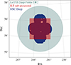 |
Fig. 1. Sky coverage of ELAIS-N1 data from LoTSS Deep Fields DR2 (∼24.5 deg2), ILT sub-arcsecond observation (∼6.7 deg2), and HSC Deep Fields (∼6.4 deg2). The holes in the HSC coverage are bright star masks. |
3.1. LoTSS Deep Fields data
LoTSS is a large radio imaging survey conducted by the LOFAR telescope with the goal of covering the entire northern sky at the frequencies ranging from 120 to 168 MHz (Shimwell et al. 2017, 2019, 2022). The LoTSS Deep Fields aims to conduct deep radio imaging over select regions, including the ELAIS-N1 field, and is able to probe fainter and higher-redshift radio sources where the dominant populations are SFGs and radio-quiet active galactic nuclei (AGNs) instead of radio-loud AGNs.
The deep-field ELAIS-N1 data we used are from the LoTSS Deep Fields Data Release 2 (Shimwell et al. 2025). With a total observing time of ∼500 hours using the LOFAR stations within the Netherlands, the image reaches a resolution of ∼6″ and an average noise level of ≲15 μJy beam−1 in the inner 5 deg2 (∼11 μJy beam−1 at the centre of the field). Direction-dependent calibration and imaging techniques (see Tasse et al. 2021) were employed during the image synthesis process in order to compensate for the direction-dependent effects (DDEs), such as ionospheric distortions. From the image, the ELAIS-N1 source catalogue was extracted with the Python Blob Detector and Source Finder2 (PYBDSF; Mohan & Rafferty 2015) where single or multiple Gaussians were fit to each detected source. The full catalogue contains 154 952 sources, with a mean source density of ∼1.8 arcmin−2 (∼2.7 arcmin−2 in the inner 5 deg2 region).
We did not use the shape information measured from this survey, as the PSF in the LoTSS Deep Fields is too large to permit accurate shape measurements for galaxies. Instead, we used the full catalogue to cross-match with the optical dataset and compute the shear correlation from the optical counterparts (see Sect. 4).
3.2. ILT data
The radio data obtained in the previous section only make use of the Dutch LOFAR stations, which have baselines up to approximately 120 km. Recently, de Jong et al. (2024) released a sub-arcsecond ELAIS-N1 image using all Dutch and international LOFAR stations, which extended the maximum baseline to around 2000 km, and thus provided a significant advantage in terms of angular resolution over the Dutch LOFAR.
The ILT sub-arcsecond data of ELAIS-N1 include four 8-hour observations and achieves a highest resolution of 0.3″. Due to the increased number of stations in ILT, the RMS noise level reaches 14 μJy beam−1 at the centre of the field, which is comparable to that of a 500-hour observation with Dutch LOFAR (see Sect. 3.1). Similar to the imaging and cataloguing processes in the 500-hour ELAIS-N1 data, the imaging process for ILT data also employs direction-dependent calibration techniques, and PYBDSF is also used for cataloguing. The full catalogue at 0.3″ resolution contains 9203 sources, and it covers a sky area of ∼6.7 deg2.
A series of cuts were applied to the catalogue to reduce the systematics for the later analysis. Sources with complex morphologies were removed by setting the source code S_Code=“S”3. Additionally, unresolved sources whose PYBDSF deconvolved major and minor axes (DC_Maj and DC_Min columns in the catalogue) were equal to zero were discarded from the catalogue. To select only the extended sources, we used a simple size cut, Maj > Maj_PSF, to reject the sources that were too small and thus were easily influenced by the point spread function (PSF). After applying these cuts, we were left with 7211 sources, corresponding to ∼78% of the full catalogue. Table 1 summarises these cuts. A large fraction of sources were preserved after these cut owing to the exceptional angular resolution attained by international LOFAR.
Summary of the cuts applied to the ILT sub-arcsecond ELAIS-N1 catalogue.
We use the PYBDSF shapes measured by ILT in Sect. 5.2 to compare the radio-optical shape. The ellipticity e for each source was calculated from the PYBDSF major axis a, minor axis b, and the position angle α,
 (8)
(8)
where we converted the PYBDSF position angle PA, measured east of north, into the angle measured north of west, which is conventionally used in weak-lensing studies. a and b are deconvolved major and minor axes. The uncertainty of the ellipticity, σe, was estimated by propagating the uncertainties of a, b, and α through the above equation. Typical measurement uncertainties for a, b, and α are  ,
,  , and
, and  . These combine to yield an effective shape measurement noise of
  per component for the ILT sample.
We did not explicitly separate AGNs and SFGs in the LoTSS and ILT samples because our selection criteria naturally result in an SFG-dominated population. An analysis of the LoTSS Deep Fields Data Release 1 (Best et al. 2023) found that ∼80% of sources are SFGs. Given the improved sensitivity in LoTSS Deep Fields Data Release 2 and ILT observations compared to LoTSS Deep Fields Data Release 1, we expect an even higher SFG fraction in our samples. In addition, by selecting only resolved sources with simple morphologies, we excluded most AGNs, which often exhibit complex structures poorly fit by Gaussian profiles. An SFG-dominated sample with simple source shapes is sufficient for the purposes of this study, although residual AGN contamination may still introduce a small model bias in the weak-lensing analysis.
3.3. HSC-SSP survey data
HSC-SSP is an ongoing multi-band imaging survey using the Hyper Suprime-Cam instrument on the Subaru 8.2m telescope (Aihara et al. 2018a). The survey consists of three layers at different depths: Wide, Deep, and UltraDeep, of which the Wide layer is specifically designed for the weak-lensing analysis, the primary science driver of the HSC-SSP survey. The ELAIS-N1 field is one of the HSC Deep layer fields. It does not lie within the Wide layer footprint and was therefore excluded in their published cosmic shear analyses (e.g. Hikage et al. 2019; Hamana et al. 2020; Dalal et al. 2023). However, we show in Sect. 4 that, benefiting from the excellent image quality, a statistically significant cosmic shear signal can be detected in this field with HSC data.
We employed the HSC-SSP S16A data release, which was made public as part of HSC-SSP second data release (see Aihara et al. 2019). This release provides photometric data in five broad bands (grizy) along with two other narrow bands for the ELAIS-N1 field. The i-band images, with the given priority in the observing strategy, have the highest image quality and were accordingly used to measure the galaxy shapes. The HSC image and catalogue data we used in this paper are the outputs from the HSC pipeline (Bosch et al. 2018).
We imposed the same galaxy selection criteria on the S16A ELAIS-N1 catalogue as in the HSC first-year (Y1) shear catalogue paper (Mandelbaum et al. 2018a). This ensured the selection of a galaxy sample with a nearly identical data quality as the Y1 shear catalogue4, which is essential to apply the HSC open-source shear calibration software5. We defined the weak-lensing full depth and full colour (WLFDFC) area for the HSC ELAIS-N1 field, requiring that the number of visits countInputs for each grizy band was larger than 3, 3, 4, 4, and 4 visits, respectively. To mask out the sources near the bright objects, we set iflags_pixel_bright_object_any=False. In addition, the i-band CModel6 magnitude of the weak-lensing sources should be lower than 24.5 AB mag after they were corrected for extinction. We refer to Sect. 5.1 or Table 4 in Mandelbaum et al. (2018a) for a full description of all the galaxy cuts.
The final HSC ELAIS-N1 weak-lensing sample contained 456 593 sources and covered a total area of 6.4 deg2, reaching a 5σ point source depth of 26.6 AB mag and mean seeing of ∼0.54 arcsec in the i band. We estimated the 5σ limiting magnitude for a point source by averaging the PSF magnitudes of stars with an S/N between 4.9 and 5.1 in the ELAIS-N1 field after applying area cuts. This estimate is considered reasonable in this field for the S16A data release, which includes 90 nights of observations, as it lies in between the i-band depths of the same field in the HSC-SSP first and second data releases. Their depths are 26.5 and 26.6 mag, respectively, with an observing time of 61.5 and 174 nights (Aihara et al. 2018b, 2019). In Fig. 2 we compare the two key sample characteristics relevant for the shear calibration: the seeing conditions and the S/N distributions between the ELAIS-N1 weak-lensing sample and the Y1 shear catalogue. The S/N distribution of the ELAIS-N1 sample (black line) resembles that of the HECTOMAP field in the Y1 shear catalogue (faint yellow line), and the seeing condition is among those in the Y1 shear catalogue. The differences are very minor, suggesting that the aforementioned shear calibration code used for the Y1 shear catalogue remains applicable to the ELAIS-N1 sample and would not cause a serious problem in the subsequent analysis. The S/Ns of the galaxies in ELAIS-N1 are in general higher than those in the Y1 shear catalogue, as shown in the top panel of Fig. 2. The former goes approximately 0.6 mag deeper on average than the latter catalogue.
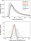 |
Fig. 2. Unweighted distributions of the i-band CModel S/N and seeing FWHM for the galaxies in the HSC ELAIS-N1 weak-lensing sample and in the six disjointed fields of the HSC Y1 shear catalogue (XMM, GAMA15H, GAMA09H, HECTOMAP, VVDS, and WIDE12H). The seeing FWHM was calculated assuming a Gaussian PSF. |
The galaxy shapes in the ELAIS-N1 weak-lensing sample were obtained using re-Gaussianisation PSF correction method based on the measurements of moments (Hirata & Seljak 2003). Following Appendix 3 of Mandelbaum et al. (2018a), the shear estimate,  , for each galaxy is defined as
 (9)
(9)
where e = (e1, e2) is the measured ellipticity, c = (c1, c2) is the additive bias, ⟨m⟩ denotes the weighted average of the multiplicative bias, with the weight given by
 (10)
(10)
where σe denotes the shape measurement error, and erms is the intrinsic shape dispersion. ℛ represents the shear response of the measured ellipticity to a small shear distortion (Kaiser et al. 1995; Bernstein & Jarvis 2002),
 (11)
(11)
The quantities in Eq. (9) are either available in the HSC public database or can be calculated from the additional data columns generated by the shear calibration software, where the shape noise and calibration factors are derived using the HSC weak-lensing simulations described in Mandelbaum et al. (2018b).
We assigned a redshift to each galaxy in the ELAIS-N1 weak-lensing sample with the best point estimate of the photometric redshift (photo-z) derived from a neural network code, EPHOR AB (see Tanaka et al. 2018). For the estimate of the redshift probability distribution function (PDF) of the sample, we employed the mathematically convenient method provided in Tanaka et al. (2018), the Gaussian kernel density estimator (KDE),
![Mathematical equation: $$ \begin{aligned} n^\mathrm{MC} (z) = \frac{1}{\sqrt{2\pi }Nh}\sum _i^N \exp \left[-\frac{(z-z_{\mathrm{MC} ,i})^2}{2h^2}\right], \end{aligned} $$](/articles/aa/full_html/2025/08/aa54446-25/aa54446-25-eq17.gif) (12)
(12)
where h = 0.05 is the kernel width for the EPHOR AB code, N denotes the total number of sample galaxies, and zMC is a Monte Carlo draw from the redshift probability distribution for each galaxy, provided in the HSC database with the column name photoz_mc. The PDF inferred by the Gaussian KDE agrees well with both the stacked photo-z PDF, a sum of all the photo-z probability distributions of individual galaxies, and the PDF obtained by reweighting the reference redshift sample, as was demonstrated in Tanaka et al. (2018).
3.4. Radio-optical cross-matching
In the ELAIS-N1 field, 99% of radio detections in the LoTSS Deep Fields DR2 survey have identified optical or near-infrared counterparts (Bisigello et al., in prep.). This matching fraction should also apply to the ILT survey, as its catalogue has already been cross-matched with LoTSS data (de Jong et al. 2024).
In this study, however, we performed a cross-matching between the radio samples and the HSC weak lensing catalogue, which only includes sources with sufficient S/N and sizes for weak-lensing measurements. Since the weak-lensing catalogue is a subset of all HSC optical detections, many radio sources remain unmatched. For both the full catalogue from LoTSS Deep Field survey and the selected samples from ILT data, we used a matching radius of 1″. Out of 57 594 radio sources in the overlapping region of the HSC and LoTSS Deep Fields, 21 845 were successfully matched. For ILT data, 2595 sources were matched out of 6259 sources in the overlapped area.
The matching fractions for LoTSS and ILT data with matched HSC sources are 38% and 41%, respectively, which are slightly lower than the matching fraction reported by SuperCLASS survey7 (Battye et al. 2020). The radio observations in the SuperCLASS survey are less sensitive than those from LoTSS or the ILT. The HSC DR1 data they used in their cross-matching analysis have a depth comparable to the HSC data employed in our study, and the lower matching fraction we report is therefore consistent with expectations.
4. Two-point shear correlation functions in the ELAIS-N1 field with HSC data
We present the shear 2pCF analysis results with the HSC optical data alone in this section. After the galaxy cuts in Sect. 3.3, the remaining galaxies had a density distribution that we show in Fig. 3. For the measurement of the shear 2pCFs, we only used the galaxies whose best-estimate redshift zB was within the range from 0.1 to 2.0, as the low-redshift sources contain little lensing signal and the sources with zB > 2 are detected with relatively low S/Ns. These galaxies were then divided into three tomographic redshift bins with bin edges [0.1, 0.6, 1.1, 2.0]. Figure 4 shows the redshift distributions of the galaxies in the three tomographic bins. The median redshifts for these tomographic bins are 0.39, 0.81, and 1.35. The overall usable galaxy number density (0.1 < zB ≤ 2.0) is 19.2 arcmin−2. More properties regarding the individual tomographic sample are listed in Table 2.
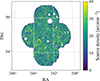 |
Fig. 3. Unweighted source density distribution of the weak-lensing sources in the ELAIS-N1 field. The unweighted mean source density for all the sources that pass the galaxy cuts in Sect. 3.3 is 19.7 arcmin−2. This plot was generated with a HEALP IX pixelisation parameter of Nside = 4096. |
Sample properties for the three tomographic bins.
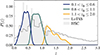 |
Fig. 4. Photometric redshift distribution. The solid lines represent the weighted redshift PDFs for the three tomographic redshift bins 0.1 < zB ≤ 0.6, 0.6 < zB ≤ 1.1, and 1.1 < zB ≤ 2.0 from the HSC weak lensing catalogue. The light grey histogram shows the weighted distribution of the best point estimates of the photometric redshift for all the HSC sources in the ELAIS-N1 weak-lensing sample. The dark grey histogram shows the redshift distribution of the LoTSS sources using photometric redshift from matched Euclid Deep Field North data. |
The shear 2pCFs can be estimated from
![Mathematical equation: $$ \begin{aligned} \hat{\xi }_\pm (\theta ) = \frac{\sum _{ij} w_i w_j\ [\hat{\gamma }_{t}(\boldsymbol{\theta }_i)\hat{\gamma }_{t}(\boldsymbol{\theta }_j) \pm \hat{\gamma }_{\times }(\boldsymbol{\theta }_i)\hat{\gamma }_{\times } (\boldsymbol{\theta }_j)]}{\sum _{ij} w_i w_j}, \end{aligned} $$](/articles/aa/full_html/2025/08/aa54446-25/aa54446-25-eq18.gif) (13)
(13)
where the summation runs over the galaxy pairs within an angular separation bin. The 2pCFs were measured in a angular range from 1′ to 80′, using the public software TREECORR (Jarvis et al. 2004). We present only the measured  in this paper because the detection of
  is not significant. In Appendix A, we show that the systematic from PSF leakage and resulting PSF contribution to the shear ξ+ is lower than 10−6, which is well below the lensing signal. As the ELAIS-N1 field is relatively small, we did not expect to achieve a very precise measurement of the shear 2pCF signal, and thus corrections for residual PSF effects were not necessary in our study. Across the full redshift range 0.1 < z ≤ 2.0, ξ+ is detected at a significance level of ∼9σ.
To determine the amplitude of the measured lensing signal, we fitted the 2pCFs with a power-law function,
 (14)
(14)
where γ is the power-law index, and θp is the pivot angular scale at which we evaluated the amplitude A of the shear correlation signal. θp was determined such that the degeneracy between parameters γ and A was minimised8. Using the galaxy samples from the two higher-redshift bins, we find θp = 3.2′ and the best-fit γ = 0.95. We then applied the power-law fitting to the three tomographic bins while keeping θp and γ fixed. The amplitudes of ξ+ for the three bins are presented in the second column of Table 3. In the redshift bins 0.6 < z ≤ 1.1 and 1.1 < z ≤ 2.0, the ξ+ amplitudes are measured with high statistical significance. Fig. 5 shows the measured 2pCFs together with the best-fit power-law functions for three redshift ranges. We note that there is a clear redshift dependence of the measured correlations, and the 2pCFs are consistent with the prediction by PYCCL9 (Chisari et al. 2019).
Amplitudes of ξ+ evaluated at θp = 3.2′ using HSC deep layer data in ELAIS-N1 field.
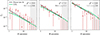 |
Fig. 5. Tomographic cosmic shear 2pCFs (red) with the power-law fitting lines (black) using a slope of γ = 0.95. The error bars were calculated from a bootstrap resampling using TREECORR. Measurements in the grey region (θ > 30′) were excluded from the fitting due to the increasing sample variance and higher contamination from PSF leakage. The green lines are theory 2pCFs from PYCCL. The best-fit χ2 values for the power-law model are indicated in the top-right corner of each panel. The 2pCF amplitudes at the angular separation θp = 3.2′ are 0.20 ± 0.15, 0.87 ± 0.10, and 1.53 ± 0.17 for 0.1 < z ≤ 0.6, 0.6 < z ≤ 1.1, and 1.1 < z ≤ 2.0, respectively. There is a clear trend that the lensing signal becomes stronger at higher redshifts. |
We also conducted a 2pCF analysis using the LoTSS-matched HSC sources. The cross-matched sample comprised 21 845 sources with a galaxy density of ∼1 arcmin−2 and a median redshift of zmed = 0.86 (see Table 4 for a comparison of summary statistics). To mitigate systematics from sample variance at large separations, our measurements were restricted to the angular separation range 1′< θ < 20′. The results are shown in the third column of Table 3. The tomographic ξ+ measurements are dominated by noise and hence are unreliable. The non-tomographic ξ+ amplitude over the redshift range 0.1 < z ≤ 2.0 reaches a significance level of ∼2σ. Notably, although the LoTSS-matched sample exhibits a higher median redshift than the HSC data, the cross-matching reduces the redshift advantage provided by the radio survey. According to host identification analysis of LoTSS sources using Euclid Deep Field North data by Bisigello et al. (in prep.), LoTSS spans a broader range of redshifts than HSC lensing samples, as shown in Fig. 4. A match with a deeper optical lensing survey would result in a higher median redshift and in an increased source count, both of which would increase the S/N. This analysis demonstrates the potential of radio surveys as deep as LoTSS for cosmic shear studies, provided the resolution were increased.
Summary statistics of radio and optical samples in the ELAIS-N1 field.
5. Comparison of radio and optical samples
5.1. Summary statistics
Table 4 summarises the properties of the samples that we selected in Sect. 3. Our main points are noted below.
-
Although the source density in LoTSS Deep Fields DR2, 1.75 arcmin−2, is relatively high for a radio survey, the majority of sources are unresolved due to the low resolution, which renders them unusable for weak-lensing measurements. In the case of ILT sub-arcsecond sources, a significant number of resolved sources are maintained (see Table 1), but the number density, 0.3 arcmin−2, remains insufficient for a reliable detection of cosmic shear. The detection of shear signal typically requires at least a few galaxies per square arcmin.
-
In the cross-matched HSC × ILT sub-arcsecond sample, the radio shape measurement noise (σe = 0.227) is approximately three times higher than the HSC shape measurement noise (σe = 0.083), but this is still lower than the intrinsic noise, and therefore, the shapes are not dominated by measurement noise.
-
The median redshifts of the HSC × LoTSS DR2 and HSC × ILT sub-arcsecond samples are both higher than that of the HSC, which highlights a potential advantage of radio weak-lensing over optical lensing.
The current low source number density and high measurement noise prevent us from conducting a weak-lensing shear analysis with LoTSS or ILT data. We place our hope in future deeper surveys, where more sources will be detected and the shape measurement noise will be significantly reduced.
5.2. Comparison of radio and optical shapes
We explored the radio-optical shape correlation using the matched ILT samples in Sect. 3.4. Since the radio emission of SFGs traces the star-forming regions, a positive correlation of the radio-optical shape is expected if the measured radio shapes in LOFAR observations are not biased by systematics.
Both HSC and LOFAR observed shapes (or shears) suffer from various systematics, with the PSF systematic being the most significant. For optical weak-lensing surveys such as HSC-SSP, the method for the shear calibration is relatively mature, and the PSF residual left in the corrected shears is usually negligible compared to the cosmic shear signal. Nonetheless, for radio observations, significant PSF contamination remains evident even after deconvolution. For instance, in ILT data, we find average ellipticity values of ⟨e1⟩= − 0.053 and ⟨e2⟩ = 0.09, which match the PSF ellipse shape (see Appendix B for ILT PSF image). Further evidence of PSF contamination is seen in the position angle distribution (Fig. 6). In this paper, we did not correct the ILT measured shapes. Because our current goal is not to conduct radio weak lensing, but to explore its capabilities with LOFAR data, a precise calibration of radio shear would bepremature.
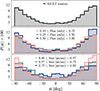 |
Fig. 6. Position angle distributions for all ILT sources (top), flux-binned sub-samples (middle), and size-binned sub-samples (bottom). The PSF contamination is present across all samples, and its strength shows a clear dependence on source size – decreasing systematically with increasing angular size. |
To examine the correlation between radio and optical shapes, we only used the radio and optical orientations (position angles) because this approach is less sensitive to the intrinsic galaxy shapes. In Fig. 7 we present the histogram of radio and optical position angles for the matched HSC × ILT sub-arcsecond sources. Evidence of positive correlation is clearly observed along the diagonal line, as well as in the ( − 90° ,90° ) and (90° , − 90° ) corners. This clear correlation in the HSC × ILT sub-arcsecond sample is also visible in the top panel of Fig. 8, where the Δα exhibits a peak at lower values and gradually decreases towards higher values. A Kolmogorov-Smirnov (KS) test against uniform distribution yields a statistic D = 0.10 with a p-value of 2 × 10⁻²¹, which clearly disagrees with a uniform distribution. We further split the sample into radio flux and radio size sub-samples and show the |Δα| distributions in the lower two panels of Fig. 8. The high-flux and large-size radio sources both exhibit position angles that are more closely aligned with their optical counterparts, with size having a stronger influence than flux.
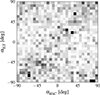 |
Fig. 7. 2D histogram of the radio and optical position angles of the cross-matched catalogue between ILT sub-arcsecond and HSC. |
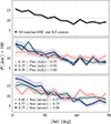 |
Fig. 8. Distributions of the absolute difference in position angles between matched ILT and HSC sources. The top panel shows the overall distribution for all matched sources. The lower panels show distributions for sub-samples divided by radio flux density (middle) and by radio size (bottom). The shaded error band reflects the Poisson uncertainties. The solid grey line represents the scenario without a correlation between the radio and optical position angles. For all matched sources, the KS statistic relative to a uniform distribution is D = 0.10. For the three increasing flux bins, the KS statistics are D = 0.06, 0.12, and 0.12. For the three increasing size bins, the KS statistics are D = 0.06, 0.10, and 0.18. In all cases, the p-values are lower than 0.005. |
Next, we provided a quantitative measure of the position angle correlation strength. Previous studies preferred to directly use the Pearson correlation coefficient of the position angle to compare radio and optical shapes (e.g. Patel et al. 2010; Tunbridge et al. 2016; Hillier et al. 2019). A linear correlation measure like this cannot fully capture the relation between spin-2 quantities such as position angles, however, due to their periodic nature. To address this limitation, we calculated the Pearson correlation coefficient between cos(2αHSC) and cos(2αILT). Alternatively, the correlation can also be evaluated using sin(2αHSC) and sin(2αILT). When the position angle α follows a uniform distribution, the correlation coefficients Rsin(2α) and Rcos(2α) are expected to be identical. Notably, in cases of strong correlation, our definition of the correlation coefficient converges to the traditionally used Pearson correlation coefficient.
We obtained Rcos(2α) = 0.15 ± 0.02, Rsin(2α) = 0.14 ± 0.02 for the matched sample, indicating a weak positive correlation. To illustrate the correlation, in Fig. 9, we present images of six selected cross-matched sources between HSC, LoTSS, and ILT. Although the ILT images lack some extended emission present in the HSC images due to limited depth, sources (a), (c), and (d) exhibit notable shape similarities between HSC and ILT. In contrast, the LoTSS sources in panel (b) and (f) appear to be two distinct sources that are blended. This underscores the necessity of using ILT observations for shape measurements and highlights its potential for future radio weak-lensing studies.
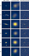 |
Fig. 9. 21″ × 21″ cutout images for six sources in the cross-matched HSC, LoTSS Deep Field DR2 and ILT sub-arcsecond catalogues of ELAIS-N1. The LoTSS Deep Field DR2 images are restored with a circular Gaussian beam with an FWHM of 6″, and the ILT sub-arcsecond images are restored with a elliptical Gaussian beam with an FWHM of 0.36″ × 0.45″. For better visualisation, the minimum and maximum pixel value are fixed to [ − 1σ, 200σ], [ − 3σ, 130σ], and [ − 3σ, 10σ] for HSC, LoTSS, and ILT data, respectively, where σ represents the background RMS noise level for each image. The PSF sizes are shown in the bottom left corner of each panel. In the HSC and ILT panels, the bottom right corner shows the source position angles. For ILT sources, we also show the standard error of the position angle in a fan-shaped patch. |
6. Forecasts for the International LOFAR Telescope
The ILT offers a significantly higher resolution than the Dutch LOFAR, enabling it to resolve sources that the Dutch array cannot. As we have shown above, however, the current ILT observations of ELAIS-N1 lack the necessary depth to be fully effective for weak-lensing studies. In this section, we assess the potential of the ILT for weak-lensing studies by considering two scenarios of deeper observations.
For both scenarios, we considered the same observing area as the ILT ELAIS-N1 data, which covers 6.7 deg2, corresponding to a single ILT pointing. Based on our successful detection of cosmic shear in a similar sky region using HSC data (Sect. 4), we anticipate that with a sufficient depth and an ILT resolution of 0.3″, a cosmic shear signal should be detectable. We explored two integrated observing times: 128 hours, and 3200 hours. A 32-hour ILT observation achieves a median RMS noise level of 17 μJy beam−1 (de Jong et al. 2024), and because the noise level is expected to scale with the inverse square root of the total observing time, we estimated the median noise levels for 128-hour and 3200-hour observations to be approximately 8.5 and 1.7 μJy beam−1, respectively.
We used the Tiered Radio Extragalactic Continuum Simulation (T-RECS; Bonaldi et al. 2018) to model the galaxy density and redshift distribution of radio populations. We employed the significance of the total flux as the detection criterion and applied a total flux cut to the raw catalogue generated by T-RECS. Assuming a 10σ detection threshold, we set the flux limits for the simulations at 85 μJy and 17 μJy for observation times of 128 hours and 3200 hours. From the simulated catalogues, we further selected sources with angular sizes greater than the PSF size10. After applying these two cuts, the mock catalogues reached source densities of 2.0 arcmin−2 for the 128-hour scenario and 6.5 arcmin−2 for the 3200-hour scenario.
For redshift distributions, we smoothed the raw z distribution from mocks (shown in Fig. 10) using the ng(z) model from Fu et al. (2008),
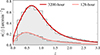 |
Fig. 10. Redshift distributions of 128-hour (green) and 3200-hour (red) mocks. The solid lines show the best-fit redshift distribution model using the n(z) parametrisation from Fu et al. (2008). The redshift bin size is 0.15. The median redshifts for the 128- and 3200-hour simulations are 0.8 and 0.9. |
 (15)
(15)
where A is a normalisation parameter. The best-fit parameters are listed in Table 5. To make a simple prediction of shear 2pCF with the mock catalogues, we assumed an intrinsic shape dispersion of erms = 0.3 per component. Since the weak-lensing 2pCF depends quadratically on the galaxy ellipticities, the noise RMS for 2pCF signal is proportional to the square of the ellipticity dispersion. In this analysis, we only considered shot noise from shape dispersion. For each bin, the noise RMS is given by
 (16)
(16)
Here, Npair(θ) is the number of galaxy pairs within a given redshift bin, derived directly from the mock catalogues. We used PYCCL to compute the theory shear 2pCFs. The weak-lensing 2pCF forecasts for the 128- and 3200-hour ILT observations are shown in Fig. 11, with the 2pCF reaching significance levels of 1.8σ and 6.8σ, respectively. Although these forecasts are optimistic because they do not account for measurement noise or systematic errors, the results suggest that weak-lensing signals from ILT radio data may be detectable, particularly with 3200-hour or deeper observations.
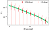 |
Fig. 11. Weak-lensing shear 2pCFs for the forecast 128- and 3200-hour ILT observations. The error bars only include shot noise. The green lines indicate the theoretical 2pCFs predicted with PYCCL using the redshift distributions in Fig. 10. |
We point out that in radio weak lensing, while increasing observation time helps to reduce measurement noise, mitigating the PSF systematics remains a major challenge. In radio interferometric imaging, the widely used CLEAN dirty-image deconvolution algorithm (Högbom 1974) performs suboptimally when applied to extended and diffuse emission because it assumes that the sources are composed of point sources. Therefore, this conventional deconvolution approach may introduce shear bias when shape information is extracted from radio data. To address these limitations, new deconvolution algorithms have been developed that are better suited for reconstructing extended sources and thereby improving image quality. Many of these advanced algorithms are computationally intensive in nature, however. Compressed sensing-based approaches (e.g. Carrillo et al. 2012, 2014; Dabbech et al. 2015) that rely on sparsity assumptions require a global optimisation, Bayesian inference methods (e.g. Junklewitz et al. 2016) involve iterative probabilistic sampling, and neural networks (e.g. Connor et al. 2022) demand extensive training. This is all significantly more computationally expensive than the simpler, local reconstruction approach of CLEAN. Ongoing efforts to balance computational efficiency with the need for precise imaging are thus essential to fully unlock the potential of radio weak lensing as a tool for probing the large-scale structure of the Universe.
7. Discussion
7.1. Trade-off between resolution and sensitivity in radio surveys
Radio interferometers detect visibilities. By applying different weighting schemes to these visibilities, we can control the characteristics of PSF in the resulting image. In general, low-resolution imaging has a better surface brightness sensitivity and is more effective at preserving extended emissions than high-resolution imaging because it prioritises measurements from shorter baselines. de Jong et al. (2024) offer ILT ELAIS-N1 catalogues at three resolutions: 0.3″, 0.6″, and 1.2″. In their analysis of integrated flux distribution across these three catalogues, they found that the 0.6″ and 1.2″ catalogues contain more detections than the 0.3″ catalogue at flux densities above ∼0.25 mJy and ∼0.55 mJy, respectively. Furthermore, around 20% of the sources detected in the 1.2″ catalogue are missing from the 0.3″ catalogue. Since most of the detected sources are expected to be SFGs at the sensitivity level of ILT ELAIS-N1 data (Best et al. 2023), it is likely that a fraction of SFGs with sizes smaller than an arcsecond account for the missing detections, as a resolution of 0.3″ tends resolve these sources out (de Jong et al. 2024).
We have used the 0.3″ resolution ELAIS-N1 catalogue because it provides the deepest map and yields the largest number of sources after selection, compared to the two lower resolutions. We also verified that this resolution does not significantly resolve out extended emission when compared to 0.6″ resolution measurements, retaining comparable shape characteristics. On average, the difference in the source position angles measured at 0.3″ and 0.6″ resolution is 24° (see Appendix C). Our choice of the 0.3″ resolution likely excluded a fraction of SFGs, however. For future radio weak-lensing studies, it might be beneficial to optimise the trade-off between resolution and surface brightness sensitivity in order to maximise the number of detected sources available for weak-lensing analysis.
7.2. Radio shape measurements
Throughout our work, we used radio shape measurements from PYBDSF. Currently, PYBDSF is the most popular software for detecting and extracting source characteristics from radio images. It is particularly well suited for detecting radio sources because it can handle the correlated noise inherent in radio images better, whereas source extraction tools widely used in optical surveys such as SEXTRACTOR (Bertin & Arnouts 1996) assume uncorrelated noise. To characterise the shapes, PYBDSF models the source flux distribution as a group of 2D Gaussians, with the intention to capture the large-scale radio emission and complex morphologies that are typically associated with radio-loud AGNs, such as jets, lobes, and hotspots.
The PYBDSF shape measurement is not ideal for weak-lensing purposes, however, because in deep radio observations, SFGs constitute the majority of the usable sources for weak lensing. SFGs often exhibit an exponential light profile, and fitting such a distribution with a 2D Gaussian can lead to systematic biases in ellipticity measurements. Moreover, the PYBDSF algorithm attempts to fit sources iteratively: It first fits a source with a single Gaussian and evaluates the residuals, and if the residual exceeds a predefined threshold, it adds additional Gaussians until an acceptable fit is achieved. As a result, high S/N SFGs are likely to be modelled with multiple Gaussians, which further complicates the accurate determination of ellipticity. In radio weak-lensing studies, where the extended emission is resolved to a certain degree, it is essential to separately measure their shapes to obtain more accurate measurements after PYBDSF identifies potential SFGs. For example, Hillier et al. (2019), Harrison et al. (2020), and Tunbridge et al. (2016) used the IM3SHAPE image-plane shape measurement method (Zuntz et al. 2013) that was originally designed for optical data in combination with a calibration for interferometric imaging artefacts to derive radio shapes for selected sources. Alternatively, shapes can be measured in the visibility domain to avoid the highly non-linear imaging process (Rivi et al. 2016; Rivi & Miller 2018). Nonetheless, these approaches have not yet been rigorously tested on real observations.
7.3. Limitations of ILT on weak lensing
In contrast to the SKA, the ILT is not designed as a survey telescope for studies of the large-scale cosmic structure. For instance, the proposed SKA Medium-Deep Band 2 Survey, which aims to study radio weak lensing, can cover approximately 5000 deg2 in 10 000 observation hours, achieving a usable source density of ∼3 sources arcmin−2 (Square Kilometre Array Cosmology Science Working Group 2020). The ILT, on the other hand, is optimised for deep, targeted observations, which limits its efficiency in achieving high source densities within short observation times. Weak-lensing studies with the ILT can only be conducted in conjunction with ultra-deep surveys.
A second potential limitation for the ILT is DDEs of radio observations, with ionospheric distortions being the most severe one for LOFAR due to its very low operating frequency. Typically, direction-dependent calibration techniques are employed to address these issues. A precise sky model is required to accurately obtain calibrated visibilities, however, especially when accounting for ionospheric effects. It is challenging to perfectly model the ionosphere, and the non-linear nature of the CLEAN deconvolution algorithm further complicates the reconstruction of the source shapes. Combined, these factors make it uncertain how significantly ionospheric effect, radio calibration, and imaging may influence the PSF systematics and thus affect the weak-lensing shape measurements.
8. Conclusions
We presented a weak-lensing analysis alongside a radio-optical shape correlation analysis conducted in the ELAIS-N1 field. Our optical data in ELAIS-N1 were taken from the HSC-SSP deep survey. We filtered the catalogue with the same cuts as in the HSC weak-lensing pipeline (Mandelbaum et al. 2018a) and found a ∼9σ detection of cosmic shear signal in the optical data via a 2pCF analysis. By dividing the lensing sources into three redshift bins, we also identified a clear signal that is indicative of its redshift dependence. This successful measurement raises the prospect of detecting similar signals using radio data on the same sources, even over relatively small sky areas.
We used two radio datasets from LOFAR in the ELAIS-N1 field: the LoTSS and ILT observations. The LoTSS survey provides the deepest low-frequency imaging of the field, with a source density reaching ∼2.7 arcmin−2 in the central region. Using LoTSS-matched HSC samples, we measured the amplitude of the shear correlation ξ+ at a ∼2σ significance level. While the LoTSS survey offers a sufficient source density for weak-lensing studies, its resolution is inadequate for precise shape measurements.
In contrast, the ILT survey delivers the highest-resolution radio imaging in ELAIS-N1 at 0.3″, but with a higher noise level than LoTSS. To access the potential of a weak-lensing analysis with ILT, we first examined the correlation between radio and optical shapes by cross-matching the ILT-detected sources with the HSC catalogue. The source position angle was used to evaluate the degree of radio-optical shape correlation. We measured a positive correlation of Rcos(2α) = 0.15 ± 0.02. High-resolution ILT observations are therefore able to begin resolving SFGs.
Currently, the ILT survey depth is insufficient to achieve the source density required for a robust cosmic shear detection. The usable source density in the ILT ELAIS-N1 field is only 0.3 arcmin−2, which is lower by over a factor of ten compared to optical surveys. Hence, we look forward to the future deeper ILT surveys and remain optimistic about the continued development of radio shear measurement techniques, which can take advantage of the high median redshift probed by radio surveys. We estimate that with 3200-hour ILT observation over a single pointing (∼6.7 deg2), a ∼6σ detection of the cosmic shear signal via 2pCF analysis could be achieved. At this depth, the source density would be adequate for weak-lensing measurements. The primary challenge lies in controlling systematic errors. The ILT observations are affected by visibility interference from ionospheric effects, which disrupts the deterministic nature of the PSF. Additionally, the non-linear nature of the radio image deconvolution process complicates the reconstruction of radio shapes. We showed in Sect. 5.2 that the shapes from ILT observations are heavily contaminated by the PSF. Mitigating these systematics and accurate radio shape measurements will be critical for future weak-lensing studies with radio data.
This criterion is imperfect for selecting simple morphologies, as some high signal-to-noise ratio (S/N) SFGs are excluded due to internal drawback in the PYBDSF code. See Sect. 7.3 for further discussion.
HSC Y1 shear catalogue is based on the Wide S16A dataset and is available for direct download from the HSC postgreSQL database. Instructions can be found here: https://hsc-release.mtk.nao.ac.jp/doc/index.php/s16a-shape-catalog-pdr2/
Composite model photometry, the primary photometry algorithm used in the HSC pipeline.
In SuperCLASS survey analysis, an matching fraction of ∼43% (∼62%) was obtained by cross-matching the e-MERLIN (JVLA) radio observations with the HSC-SSP DR1 weak lensing catalogue. The noise levels for the e-MERLIN and JVLA observations are 7 μJy beam−1 at L-band (1.4 GHz). When converted to the equivalent noise level at 150 MHz, using a spectral index of 0.7, this corresponds to approximately 33 μJy beam−1.
This was done by tuning θp and minimising the covariance between γ and A.
We set the PSF size to 0.4″, which corresponds to the geometric mean of the major and minor axes of the elliptical PSF from the 32-hour ILT ELAIS-N1 observation.
Acknowledgments
We thank Hironao Miyatake for helpful advice on using the HSC data products. We thank George Miley, Jurjen de Jong, Timothy Shimwell for their helpful discussions. We thank the anonymous referee for their helpful comments and suggestions. JL is supported by the funding from China Scholarship Council (CSC) under the Agreement for Study Abroad for CSC Sponsored Chinese Citizens No 202206040036. The Hyper Suprime-Cam (HSC) collaboration includes the astronomical communities of Japan and Taiwan, and Princeton University. The HSC instrumentation and software were developed by the National Astronomical Observatory of Japan (NAOJ), the Kavli Institute for the Physics and Mathematics of the Universe (Kavli IPMU), the University of Tokyo, the High Energy Accelerator Research Organization (KEK), the Academia Sinica Institute for Astronomy and Astrophysics in Taiwan (ASIAA), and Princeton University. Funding was contributed by the FIRST program from the Japanese Cabinet Office, the Ministry of Education, Culture, Sports, Science and Technology (MEXT), the Japan Society for the Promotion of Science (JSPS), Japan Science and Technology Agency (JST), the Toray Science Foundation, NAOJ, Kavli IPMU, KEK, ASIAA, and Princeton University. This paper makes use of software developed for Vera C. Rubin Observatory. We thank the Rubin Observatory for making their code available as free software at http://pipelines.lsst.io/. This paper is based on data collected at the Subaru Telescope and retrieved from the HSC data archive system, which is operated by the Subaru Telescope and Astronomy Data Center (ADC) at NAOJ. Data analysis was in part carried out with the cooperation of Center for Computational Astrophysics (CfCA), NAOJ. We are honoured and grateful for the opportunity of observing the Universe from Maunakea, which has the cultural, historical and natural significance in Hawaii. LOFAR (van Haarlem et al. 2013) is the Low Frequency Array designed and constructed by ASTRON. It has observing, data processing, and data storage facilities in several countries, which are owned by various parties (each with their own funding sources), and that are collectively operated by the ILT foundation under a joint scientific policy. The ILT resources have benefited from the following recent major funding sources: CNRS-INSU, Observatoire de Paris and Université d’Orléans, France; BMBF, MIWF-NRW, MPG, Germany; Science Foundation Ireland (SFI), Department of Business, Enterprise and Innovation (DBEI), Ireland; NWO, The Netherlands; The Science and Technology Facilities Council, UK; Ministry of Science and Higher Education, Poland; The Istituto Nazionale di Astrofisica (INAF), Italy. The data analysis was carried out with the use of MOCPY (Fernique et al. 2014), HEALPIX (Górski et al. 2005; Zonca et al. 2019), NUMPY (Harris et al. 2020), SCIPY (Virtanen et al. 2020), PANDAS (McKinney 2010; The pandas development team 2020), ASTROPY (Astropy Collaboration 2013, 2018, 2022), and MATPLOTLIB (Hunter 2007).
References
- Abbott, T. M. C., Abdalla, F. B., Alarcon, A., et al. 2018, Phys. Rev. D, 98, 043526 [NASA ADS] [CrossRef] [Google Scholar]
- Aihara, H., Arimoto, N., Armstrong, R., et al. 2018a, PASJ, 70, S4 [NASA ADS] [Google Scholar]
- Aihara, H., Armstrong, R., Bickerton, S., et al. 2018b, PASJ, 70, S8 [NASA ADS] [Google Scholar]
- Aihara, H., AlSayyad, Y., Ando, M., et al. 2019, PASJ, 71, 114 [Google Scholar]
- Amendola, L., Appleby, S., Avgoustidis, A., et al. 2018, Liv. Rev. Relat., 21, 2 [Google Scholar]
- Astropy Collaboration (Robitaille, T. P., et al.) 2013, A&A, 558, A33 [NASA ADS] [CrossRef] [EDP Sciences] [Google Scholar]
- Astropy Collaboration (Price-Whelan, A. M., et al.) 2018, AJ, 156, 123 [Google Scholar]
- Astropy Collaboration (Price-Whelan, A. M., et al.) 2022, ApJ, 935, 167 [NASA ADS] [CrossRef] [Google Scholar]
- Bartelmann, M., & Schneider, P. 2001, Phys. Rep., 340, 291 [Google Scholar]
- Battye, R. A., Brown, M. L., Casey, C. M., et al. 2020, MNRAS, 495, 1706 [Google Scholar]
- Becker, R. H., White, R. L., & Helfand, D. J. 1995, ApJ, 450, 559 [Google Scholar]
- Bernstein, G. M., & Jarvis, M. 2002, AJ, 123, 583 [NASA ADS] [CrossRef] [Google Scholar]
- Bertin, E., & Arnouts, S. 1996, A&AS, 117, 393 [NASA ADS] [CrossRef] [EDP Sciences] [Google Scholar]
- Best, P. N., Kondapally, R., Williams, W. L., et al. 2023, MNRAS, 523, 1729 [NASA ADS] [CrossRef] [Google Scholar]
- Bonaldi, A., Harrison, I., Camera, S., & Brown, M. L. 2016, MNRAS, 463, 3686 [Google Scholar]
- Bonaldi, A., Bonato, M., Galluzzi, V., et al. 2018, MNRAS, 482, 2 [Google Scholar]
- Bosch, J., Armstrong, R., Bickerton, S., et al. 2018, PASJ, 70, S5 [Google Scholar]
- Brown, M. L., & Battye, R. A. 2011, MNRAS, 410, 2057 [Google Scholar]
- Brown, M., Bacon, D., Camera, S., et al. 2015, Advancing Astrophysics with the Square Kilometre Array (AASKA14), 23 [Google Scholar]
- Camera, S., Harrison, I., Bonaldi, A., & Brown, M. L. 2017, MNRAS, 464, 4747 [NASA ADS] [CrossRef] [Google Scholar]
- Carrillo, R. E., McEwen, J. D., & Wiaux, Y. 2012, MNRAS, 426, 1223 [Google Scholar]
- Carrillo, R. E., McEwen, J. D., & Wiaux, Y. 2014, MNRAS, 439, 3591 [Google Scholar]
- Chang, T.-C., Refregier, A., & Helfand, D. J. 2004, ApJ, 617, 794 [Google Scholar]
- Chisari, N. E., Alonso, D., Krause, E., et al. 2019, ApJS, 242, 2 [Google Scholar]
- Connor, L., Bouman, K. L., Ravi, V., & Hallinan, G. 2022, MNRAS, 514, 2614 [NASA ADS] [CrossRef] [Google Scholar]
- Dabbech, A., Ferrari, C., Mary, D., et al. 2015, A&A, 576, A7 [CrossRef] [EDP Sciences] [Google Scholar]
- Dalal, R., Li, X., Nicola, A., et al. 2023, Phys. Rev. D, 108, 123519 [CrossRef] [Google Scholar]
- de Jong, J. T. A., Verdoes Kleijn, G. A., Kuijken, K. H., & Valentijn, E. A. 2013, Exp. Astron., 35, 25 [Google Scholar]
- de Jong, J. M. G. H. J., van Weeren, R. J., Sweijen, F., et al. 2024, A&A, 689, A80 [NASA ADS] [CrossRef] [EDP Sciences] [Google Scholar]
- Demetroullas, C., & Brown, M. L. 2016, MNRAS, 456, 3100 [Google Scholar]
- Demetroullas, C., & Brown, M. L. 2018, MNRAS, 473, 937 [Google Scholar]
- Euclid Collaboration (Mellier, Y., et al.) 2025, A&A, 697, A1 [Google Scholar]
- Fernique, P., Boch, T., Donaldson, T., et al. 2014, MOC – HEALPix Multi-Order Coverage map Version 1.0, IVOA Recommendation 02 June 2014 [Google Scholar]
- Fu, L., Semboloni, E., Hoekstra, H., et al. 2008, A&A, 479, 9 [NASA ADS] [CrossRef] [EDP Sciences] [Google Scholar]
- Gatti, M., Sheldon, E., Amon, A., et al. 2021, MNRAS, 504, 4312 [NASA ADS] [CrossRef] [Google Scholar]
- Giblin, B., Heymans, C., Asgari, M., et al. 2021, A&A, 645, A105 [NASA ADS] [CrossRef] [EDP Sciences] [Google Scholar]
- Górski, K. M., Hivon, E., Banday, A. J., et al. 2005, ApJ, 622, 759 [Google Scholar]
- Hamana, T., Shirasaki, M., Miyazaki, S., et al. 2020, PASJ, 72, 16 [Google Scholar]
- Harris, C. R., Millman, K. J., van der Walt, S. J., et al. 2020, Nature, 585, 357 [NASA ADS] [CrossRef] [Google Scholar]
- Harrison, I., Camera, S., Zuntz, J., & Brown, M. L. 2016, MNRAS, 463, 3674 [Google Scholar]
- Harrison, I., Brown, M. L., Tunbridge, B., et al. 2020, MNRAS, 495, 1737 [Google Scholar]
- Heymans, C., Van Waerbeke, L., Miller, L., et al. 2012, MNRAS, 427, 146 [Google Scholar]
- Hikage, C., Oguri, M., Hamana, T., et al. 2019, PASJ, 71, 43 [Google Scholar]
- Hillier, T., Brown, M. L., Harrison, I., & Whittaker, L. 2019, MNRAS, 488, 5420 [Google Scholar]
- Hirata, C., & Seljak, U. 2003, MNRAS, 343, 459 [Google Scholar]
- Högbom, J. A. 1974, A&AS, 15, 417 [Google Scholar]
- Hunter, J. D. 2007, Comput. Sci. Eng., 9, 90 [NASA ADS] [CrossRef] [Google Scholar]
- Ivezić, Ž., Kahn, S. M., Tyson, J. A., et al. 2019, ApJ, 873, 111 [Google Scholar]
- Jarvis, M., Bernstein, G., & Jain, B. 2004, MNRAS, 352, 338 [Google Scholar]
- Junklewitz, H., Bell, M. R., Selig, M., & Enßlin, T. A. 2016, A&A, 586, A76 [NASA ADS] [CrossRef] [EDP Sciences] [Google Scholar]
- Kaiser, N., Squires, G., & Broadhurst, T. 1995, ApJ, 449, 460 [Google Scholar]
- Kilbinger, M. 2015, Rep. Progr. Phys., 78, 086901 [Google Scholar]
- Kondapally, R., Best, P. N., Hardcastle, M. J., et al. 2021, A&A, 648, A3 [EDP Sciences] [Google Scholar]
- Kuijken, K., Heymans, C., Hildebrandt, H., et al. 2015, MNRAS, 454, 3500 [Google Scholar]
- Laureijs, R., Amiaux, J., Arduini, S., et al. 2011, ArXiv e-prints [arXiv:1110.3193] [Google Scholar]
- Limber, D. N. 1953, ApJ, 117, 134 [NASA ADS] [CrossRef] [Google Scholar]
- Mandelbaum, R., Miyatake, H., Hamana, T., et al. 2018a, PASJ, 70, S25 [Google Scholar]
- Mandelbaum, R., Lanusse, F., Leauthaud, A., et al. 2018b, MNRAS, 481, 3170 [NASA ADS] [CrossRef] [Google Scholar]
- McKinney, W. 2010, in Proceedings of the 9th Python in Science Conference, eds. S. van der Walt, & J. Millman, 56 [Google Scholar]
- Mohan, N., & Rafferty, D. 2015, Astrophysics Source Code Library [record ascl:1502.007] [Google Scholar]
- Morabito, L. K., Sweijen, F., Radcliffe, J. F., et al. 2022, MNRAS, 515, 5758 [NASA ADS] [CrossRef] [Google Scholar]
- Oliver, S., Rowan-Robinson, M., Alexander, D. M., et al. 2000, MNRAS, 316, 749 [Google Scholar]
- Patel, P., Bacon, D. J., Beswick, R. J., Muxlow, T. W. B., & Hoyle, B. 2010, MNRAS, 401, 2572 [Google Scholar]
- Rivi, M., & Miller, L. 2018, MNRAS, 476, 2053 [Google Scholar]
- Rivi, M., Miller, L., Makhathini, S., & Abdalla, F. B. 2016, MNRAS, 463, 1881 [Google Scholar]
- Sabater, J., Best, P. N., Tasse, C., et al. 2021, A&A, 648, A2 [EDP Sciences] [Google Scholar]
- Shimwell, T. W., Röttgering, H. J. A., Best, P. N., et al. 2017, A&A, 598, A104 [NASA ADS] [CrossRef] [EDP Sciences] [Google Scholar]
- Shimwell, T. W., Tasse, C., Hardcastle, M. J., et al. 2019, A&A, 622, A1 [NASA ADS] [CrossRef] [EDP Sciences] [Google Scholar]
- Shimwell, T. W., Hardcastle, M. J., Tasse, C., et al. 2022, A&A, 659, A1 [NASA ADS] [CrossRef] [EDP Sciences] [Google Scholar]
- Shimwell, T. W., Hale, C. L., Best, P. N., et al. 2025, A&A, 695, A80 [NASA ADS] [CrossRef] [EDP Sciences] [Google Scholar]
- Square Kilometre Array Cosmology Science Working Group (Bacon, D. J., et al.) 2020, PASA, 37, e007 [Google Scholar]
- Sweijen, F., van Weeren, R. J., Röttgering, H. J. A., et al. 2022, Nat. Astron., 6, 350 [NASA ADS] [CrossRef] [Google Scholar]
- Tanaka, M., Coupon, J., Hsieh, B.-C., et al. 2018, PASJ, 70, S9 [Google Scholar]
- Tasse, C., Shimwell, T., Hardcastle, M. J., et al. 2021, A&A, 648, A1 [EDP Sciences] [Google Scholar]
- The Dark Energy Survey Collaboration 2005, ArXiv e-prints [arXiv:astro-ph/0510346] [Google Scholar]
- The pandas development team 2020, https://doi.org/10.5281/zenodo.3509134 [Google Scholar]
- Tunbridge, B., Harrison, I., & Brown, M. L. 2016, MNRAS, 463, 3339 [NASA ADS] [CrossRef] [Google Scholar]
- van Haarlem, M. P., Wise, M. W., Gunst, A. W., et al. 2013, A&A, 556, A2 [NASA ADS] [CrossRef] [EDP Sciences] [Google Scholar]
- Virtanen, P., Gommers, R., Oliphant, T. E., et al. 2020, Nat. Meth., 17, 261 [Google Scholar]
- White, R. L., Becker, R. H., Helfand, D. J., & Gregg, M. D. 1997, ApJ, 475, 479 [Google Scholar]
- Zonca, A., Singer, L., Lenz, D., et al. 2019, J. Open Source Softw., 4, 1298 [Google Scholar]
- Zuntz, J., Kacprzak, T., Voigt, L., et al. 2013, MNRAS, 434, 1604 [NASA ADS] [CrossRef] [Google Scholar]
Appendix A: PSF leakage in HSC ELAIS-N1 data
To estimate the PSF systematics in the HSC shear data, we assume a linear model for the systematic introduced by the PSF leakage,
 (A.1)
(A.1)
where γp is the ellipticity of the model PSF and α is a parameter that quantifies the extent of leakage. We can estimate α from the cross-correlation between the galaxy and PSF shapes ξ+gp,
 (A.2)
(A.2)
where ξ+pp is the auto-correlation of the PSF ellipticity. We use the galaxies from all three tomographic bins to calculate the quantities needed above. The measured ξ+gp and ξ+pp are shown in the top panel of Fig. A.1. The bottom panel of Fig. A.1 shows the calculated α values as a function of scale. Since α is not a scale-dependent parameter, we take the average value and its standard deviation as an final estimation of α, which leads to α = 0.021 ± 0.007. Based on this parameter, the systematic from the PSF leakage can be estimated from
 (A.3)
(A.3)
Within the angular range from 1′ to 30′, the average value for  is ∼5.7 × 10⁻⁷, which is more than two orders of magnitude smaller than the detected lensing signal in Sect. 4.
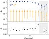 |
Fig. A.1. Estimation of the PSF leakage parameter α. Top panel shows the cross-correlation between galaxy and PSF shapes (ξ+gp), and auto-correlation of the PSF shapes (ξ+pp), where the error bars are calculated from bootstrapping. The bottom panel shows the calculated α at each angular scale. Data points in grey region are not included in the final estimation of the mean value of α. |
Appendix B: LOFAR PSFs
For radio telescopes, the shape of the PSF on the image plane depends mainly on the radio array distribution and integrated observing time. It is in principle highly deterministic. Nonetheless, for LOFAR telescope which operates at low radio frequencies, the turbulence in the Earth’s ionosphere would distort the radio emission and smear the radio image. To resolve this issue caused by ionospheric effects, a special technique called direction-dependent calibration was employed while generating the clean images in the LoTSS surveys used in this paper. This technique involves first dividing the dirty image into multiple facet images, each of which is then calibrated and deconvolved separately using its own facet PSF. In Fig. B.1, we show the PSFs from the facets that are closest to the primary beam centre. Figure B.2 shows the cross-sections of the LOFAR PSFs. Compared to PSFs in optical surveys, which usually can be well modelled by simple Gaussians to first order, the radio PSFs have some secondary structures caused by radio side lobes.
There are slight variations among the PSFs across different facets, as shown in Fig. B.3. While the PSF ellipticities are generally aligned in direction, small differences are evident both in orientation and ellipticity magnitude.
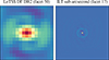 |
Fig. B.1. PSF images for ELAIS-N1 field data obtained with LoTSS Deep Fields DR2 (left), and LoTSS high resolution (right). The image size is 26″ × 26″. For colour scale, the maximum and minimum pixel values are set to 1 and −1. |
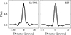 |
Fig. B.2. PSF profiles for LoTSS Deep Fields DR2 (left) and LoTSS high resolution (right). The corresponding facets of the PSFs are the same as those in Fig. B.1. Radio observations are conducted in the visibility domain, which selects a range of Fourier modes and results in the wiggling of the PSF tail around zero. |
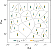 |
Fig. B.3. PSF ellipticity (green) and average source ellipticity (yellow) distributions across 30 facets in the ELAIS-N1 field from ILT observations. A clear alignment is observed between source and PSF ellipticities. |
Appendix C: ILT source shapes at lower resolution
As mentioned in Sect. 7.1, high-resolution radio imaging can resolve out extended emission. This effect may bias the shape measurements obtained from the highest available ILT resolution of 0.3″. In this section, we examine ILT source shapes derived from the lower resolution, compare them with those obtained at 0.3″, and assess whether our choice of ILT resolution adequately preserves the shape information. We use the ILT 0.6″ data as the lower-resolution reference. ILT 1.2″ data are excluded from this comparison due to its lower detection sensitivity and more elongated PSF.
We begin with a visual comparison of source shapes. Figure 9 in Sect. 5 presents 0.3″ ILT cutouts for six representative sources, with corresponding 0.6″ cutouts shown in Fig. C.1. Position angles measured at the two resolutions are generally consistent, with 0.6″ values differing from those at 0.3″ by 6.8°, 25.2°, 23.8°, 3.7°, 22.9°, -0.6° for sources (a) to (f). Notably, source (c) exhibits more pronounced extended emission in the 0.6″ image, with its position angle aligning more closely with that derived from the corresponding HSC image.
We further compare the total flux and position angles of 6 022 sources matched between the 0.3″ sample selected in Sect. 3.2 and the full 0.6″ sample. Approximately 83% of the 0.3″ sources are also detected in the 0.6″ low-resolution images. The undetected sources are typically too faint in the low-resolution data to be confirmed as reliable detections. We find the total flux in the 0.6″ data is ∼2% higher than in the 0.3″ data on average. Besides, the average absolute difference in position angles is 24°, which is smaller than the position angle uncertainties. The Pearson correlation between the position angles at two resolutions is Rcos(2α) = 0.52 ± 0.01.
These results show that 0.3″ images preserve comparable shape information from 0.6″. Using the 0.6″ resolution would not yield significantly different results in this study.
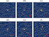 |
Fig. C.1. 21″ × 21″ cutout images of the same sources shown in Fig. 9, now displayed at ILT 0.6″ resolution. The PSF has a size of 0.58″ × 0.62″ and is shown in the bottom-left corner of each panel. The maximum and minimum pixel values are fixed to −3σ and 10σ. The standard error of the position angle is shown in the bottom-right corner of each panel in a fan-shaped patch. |
All Tables
Amplitudes of ξ+ evaluated at θp = 3.2′ using HSC deep layer data in ELAIS-N1 field.
All Figures
|
Fig. 1. Sky coverage of ELAIS-N1 data from LoTSS Deep Fields DR2 (∼24.5 deg2), ILT sub-arcsecond observation (∼6.7 deg2), and HSC Deep Fields (∼6.4 deg2). The holes in the HSC coverage are bright star masks. |
| In the text | |
|
Fig. 2. Unweighted distributions of the i-band CModel S/N and seeing FWHM for the galaxies in the HSC ELAIS-N1 weak-lensing sample and in the six disjointed fields of the HSC Y1 shear catalogue (XMM, GAMA15H, GAMA09H, HECTOMAP, VVDS, and WIDE12H). The seeing FWHM was calculated assuming a Gaussian PSF. |
| In the text | |
|
Fig. 3. Unweighted source density distribution of the weak-lensing sources in the ELAIS-N1 field. The unweighted mean source density for all the sources that pass the galaxy cuts in Sect. 3.3 is 19.7 arcmin−2. This plot was generated with a HEALP IX pixelisation parameter of Nside = 4096. |
| In the text | |
|
Fig. 4. Photometric redshift distribution. The solid lines represent the weighted redshift PDFs for the three tomographic redshift bins 0.1 < zB ≤ 0.6, 0.6 < zB ≤ 1.1, and 1.1 < zB ≤ 2.0 from the HSC weak lensing catalogue. The light grey histogram shows the weighted distribution of the best point estimates of the photometric redshift for all the HSC sources in the ELAIS-N1 weak-lensing sample. The dark grey histogram shows the redshift distribution of the LoTSS sources using photometric redshift from matched Euclid Deep Field North data. |
| In the text | |
|
Fig. 5. Tomographic cosmic shear 2pCFs (red) with the power-law fitting lines (black) using a slope of γ = 0.95. The error bars were calculated from a bootstrap resampling using TREECORR. Measurements in the grey region (θ > 30′) were excluded from the fitting due to the increasing sample variance and higher contamination from PSF leakage. The green lines are theory 2pCFs from PYCCL. The best-fit χ2 values for the power-law model are indicated in the top-right corner of each panel. The 2pCF amplitudes at the angular separation θp = 3.2′ are 0.20 ± 0.15, 0.87 ± 0.10, and 1.53 ± 0.17 for 0.1 < z ≤ 0.6, 0.6 < z ≤ 1.1, and 1.1 < z ≤ 2.0, respectively. There is a clear trend that the lensing signal becomes stronger at higher redshifts. |
| In the text | |
|
Fig. 6. Position angle distributions for all ILT sources (top), flux-binned sub-samples (middle), and size-binned sub-samples (bottom). The PSF contamination is present across all samples, and its strength shows a clear dependence on source size – decreasing systematically with increasing angular size. |
| In the text | |
|
Fig. 7. 2D histogram of the radio and optical position angles of the cross-matched catalogue between ILT sub-arcsecond and HSC. |
| In the text | |
|
Fig. 8. Distributions of the absolute difference in position angles between matched ILT and HSC sources. The top panel shows the overall distribution for all matched sources. The lower panels show distributions for sub-samples divided by radio flux density (middle) and by radio size (bottom). The shaded error band reflects the Poisson uncertainties. The solid grey line represents the scenario without a correlation between the radio and optical position angles. For all matched sources, the KS statistic relative to a uniform distribution is D = 0.10. For the three increasing flux bins, the KS statistics are D = 0.06, 0.12, and 0.12. For the three increasing size bins, the KS statistics are D = 0.06, 0.10, and 0.18. In all cases, the p-values are lower than 0.005. |
| In the text | |
|
Fig. 9. 21″ × 21″ cutout images for six sources in the cross-matched HSC, LoTSS Deep Field DR2 and ILT sub-arcsecond catalogues of ELAIS-N1. The LoTSS Deep Field DR2 images are restored with a circular Gaussian beam with an FWHM of 6″, and the ILT sub-arcsecond images are restored with a elliptical Gaussian beam with an FWHM of 0.36″ × 0.45″. For better visualisation, the minimum and maximum pixel value are fixed to [ − 1σ, 200σ], [ − 3σ, 130σ], and [ − 3σ, 10σ] for HSC, LoTSS, and ILT data, respectively, where σ represents the background RMS noise level for each image. The PSF sizes are shown in the bottom left corner of each panel. In the HSC and ILT panels, the bottom right corner shows the source position angles. For ILT sources, we also show the standard error of the position angle in a fan-shaped patch. |
| In the text | |
|
Fig. 10. Redshift distributions of 128-hour (green) and 3200-hour (red) mocks. The solid lines show the best-fit redshift distribution model using the n(z) parametrisation from Fu et al. (2008). The redshift bin size is 0.15. The median redshifts for the 128- and 3200-hour simulations are 0.8 and 0.9. |
| In the text | |
|
Fig. 11. Weak-lensing shear 2pCFs for the forecast 128- and 3200-hour ILT observations. The error bars only include shot noise. The green lines indicate the theoretical 2pCFs predicted with PYCCL using the redshift distributions in Fig. 10. |
| In the text | |
|
Fig. A.1. Estimation of the PSF leakage parameter α. Top panel shows the cross-correlation between galaxy and PSF shapes (ξ+gp), and auto-correlation of the PSF shapes (ξ+pp), where the error bars are calculated from bootstrapping. The bottom panel shows the calculated α at each angular scale. Data points in grey region are not included in the final estimation of the mean value of α. |
| In the text | |
|
Fig. B.1. PSF images for ELAIS-N1 field data obtained with LoTSS Deep Fields DR2 (left), and LoTSS high resolution (right). The image size is 26″ × 26″. For colour scale, the maximum and minimum pixel values are set to 1 and −1. |
| In the text | |
|
Fig. B.2. PSF profiles for LoTSS Deep Fields DR2 (left) and LoTSS high resolution (right). The corresponding facets of the PSFs are the same as those in Fig. B.1. Radio observations are conducted in the visibility domain, which selects a range of Fourier modes and results in the wiggling of the PSF tail around zero. |
| In the text | |
|
Fig. B.3. PSF ellipticity (green) and average source ellipticity (yellow) distributions across 30 facets in the ELAIS-N1 field from ILT observations. A clear alignment is observed between source and PSF ellipticities. |
| In the text | |
|
Fig. C.1. 21″ × 21″ cutout images of the same sources shown in Fig. 9, now displayed at ILT 0.6″ resolution. The PSF has a size of 0.58″ × 0.62″ and is shown in the bottom-left corner of each panel. The maximum and minimum pixel values are fixed to −3σ and 10σ. The standard error of the position angle is shown in the bottom-right corner of each panel in a fan-shaped patch. |
| In the text | |
Current usage metrics show cumulative count of Article Views (full-text article views including HTML views, PDF and ePub downloads, according to the available data) and Abstracts Views on Vision4Press platform.
Data correspond to usage on the plateform after 2015. The current usage metrics is available 48-96 hours after online publication and is updated daily on week days.
Initial download of the metrics may take a while.