| Issue |
A&A
Volume 700, August 2025
|
|
|---|---|---|
| Article Number | A39 | |
| Number of page(s) | 15 | |
| Section | Stellar structure and evolution | |
| DOI | https://doi.org/10.1051/0004-6361/202554633 | |
| Published online | 01 August 2025 | |
Asteroseismology of the G8 subgiant β Aquilae with SONG-Tenerife, SONG-Australia and TESS
1
Stellar Astrophysics Centre, Department of Physics and Astronomy, Aarhus University, DK-8000 Aarhus C, Denmark
2
Sydney Institute for Astronomy, School of Physics, University of Sydney, NSW 2006, Australia
3
Institute for Astronomy, University of Hawai‘i, 2680 Woodlawn Drive, Honolulu, HI 96822, USA
4
Centre for Astrophysics, University of Southern Queensland, Toowoomba, QLD 4350, Australia
5
School of Physics, University of New South Wales, NSW 2052, Australia
6
School of Physical and Chemical Sciences, Te Kura Matū, University of Canterbury, Christchurch, 8140 Aotearoa, New Zealand
7
Instituto de Astrofísica de Canarias, 38200 La Laguna, Tenerife, Spain
8
Departamento de Astrofísica, Universidad de La Laguna (ULL), 38206 La Laguna, Tenerife, Spain
9
Landessternwarte, Zentrum für Astronomie der Universität Heidelberg, Königstuhl 12, 69117 Heidelberg, Germany
10
Research School of Astronomy and Astrophysics, Australian National University, Canberra, ACT 2611, Australia
11
School of Physics and Astronomy, Monash University, Clayton, Australia
⋆ Corresponding author: This email address is being protected from spambots. You need JavaScript enabled to view it.
Received:
19
March
2025
Accepted:
13
June
2025
Abstract
Aims. We present time-series radial velocities of the G8 subgiant star β Aql obtained in 2022 and 2023 using SONG-Tenerife and, for the first time, SONG-Australia. We also analyse a sector of TESS photometry that overlapped with the 2022 SONG data.
Methods. We processed the time series to assign weights and to remove bad data points. The resulting power spectrum clearly shows solar-like oscillations centred at 430 μHz. The TESS light curve shows the oscillations at lower signal-to-noise, reflecting the fact that photometric measurements are much more affected by the granulation background than are radial velocities.
Results. The simultaneous observations in velocity and photometry represent the best such measurements for any star apart from the Sun. They allowed us to measure the ratio between the bolometric photometric amplitude and the velocity amplitude to be 26.6 ± 3.1 ppm/ms−1. We measured this ratio for the Sun from published SOHO data to be 19.5 ± 0.7 ppm/ms−1 and, after accounting for the difference in effective temperatures of β Aql and the Sun, these values align with expectations. In both the Sun and β Aql, the photometry-to-velocity ratio appears to be a function of frequency. We also measured the phase shift of the oscillations in β Aql between SONG and TESS to be −113° ±7°, which agrees with the value for the Sun and also with a 3D simulation of a star with similar properties to β Aql. Importantly for exoplanet searches, we argue that simultaneous photometry can be used to predict the contribution of oscillations to radial velocities. We measured frequencies for 22 oscillation modes in β Aql and carried out asteroseismic modelling, yielding an excellent fit to the frequencies. We derived accurate values for the mass and age, and were able to place quite strong constraints on the mixing-length parameter. Finally, we show that the oscillation properties of β Aql are very similar to stars in the open cluster M67.
Key words: stars: oscillations
© The Authors 2025
 Open Access article, published by EDP Sciences, under the terms of the Creative Commons Attribution License (https://creativecommons.org/licenses/by/4.0), which permits unrestricted use, distribution, and reproduction in any medium, provided the original work is properly cited.
This article is published in open access under the Subscribe to Open model. This email address is being protected from spambots. You need JavaScript enabled to view it. to support open access publication.
1. Introduction
Before the era of space photometry, most detections of solar-like oscillations were made with radial-velocity measurements (see reviews by Bedding & Kjeldsen 2003; Elsworth & Thompson 2004; Cunha et al. 2007; Aerts et al. 2008, 2010; Bedding et al. 2014). Starting in 2009, asteroseismology of solar-like oscillations underwent a revolution thanks to the photometric space missions CoRoT, Kepler and TESS (see reviews by Chaplin & Miglio 2013; García & Ballot 2019; Jackiewicz 2021). These space missions have provided long and nearly uninterrupted light curves with exquisite photometric precision for thousands of stars.
Importantly, measurements of solar-like oscillations with space-based photometry are usually limited by the intrinsic noise from the stars themselves, which arises from photometric fluctuations caused by surface granulation (e.g. Chaplin et al. 2011; Karoff et al. 2013; Samadi et al. 2013; Kallinger et al. 2014; Campante et al. 2016; Pande et al. 2018; Rodríguez Díaz et al. 2022). Radial velocity (RV) measurements are much less affected because the granulation background is much weaker relative to the oscillations than in photometry (Harvey 1988; Grundahl et al. 2007; Kjeldsen & Bedding 2011; Luhn et al. 2025). Indeed, recent observations with the VLT and Keck have shown that RV observations can measure the low-amplitude oscillations of K dwarfs in only a few nights (Campante et al. 2024; Hon et al. 2024; Lundkvist et al. 2024; Li et al. 2025). On the other hand, RV observations with ground-based telescopes will inevitably have gaps in the time series that compromise oscillation measurements, and the benefits of having two or more telescopes are well established (e.g. Arentoft et al. 2014).
The primary aim of SONG (Stellar Observations Network Group) is to collect high-precision RV measurements of oscillating stars. The first node at Observatorio del Teide on Tenerife, Spain, has been operating since 2014 and consists of the 1-m Hertzsprung SONG Telescope and a coudé échelle spectrograph with an iodine cell (Grundahl et al. 2007; Andersen et al. 2014, 2016). In this paper, we present SONG results that include a new node in Australia, at Mount Kent Observatory near Toowoomba in Queensland. SONG-Australia comprises two 0.7-m telescopes that are identical to those used by the MINERVA-Australis facility on the same site (Addison et al. 2019). Fibres from the two SONG telescopes are fed to a high-resolution spectrograph, equipped with an iodine cell, that is similar to the one at SONG-Tenerife.
The target for these observations was the bright G8 subgiant β Aquilae. This star is particularly interesting because it is in transition from a subgiant to a red giant. Our analysis combines RV observations from the SONG nodes in Tenerife and Australia with photometry from TESS.
2. Properties of β Aql
The G8 subgiant β Aql (HR 7602; HD 188512; HIP 98036; TIC 375621179) is a Gaia benchmark star (Soubiran et al. 2024). Its angular diameter has been measured by interferometry using both VLTI/PIONIER (Rains et al. 2020) and CHARA/PAVO (Karovicova et al. 2022), giving angular diameters (corrected for limb darkening) of 2.133 ± 0.012 mas and 2.096 ± 0.014 mas, respectively, and the effective temperature as 5071 ± 37 K and 5113 ± 20 K. For this work we adopt the mean of these two temperatures with a conservative error bar: Teff = 5092 ± 50 K. This agrees with the spectroscopic value of Teff = 5030 ± 80 K measured by Bruntt et al. (2010). Those authors reported a metallicity for β Aql of [Fe/H] = −0.21 ± 0.07, which we adopt for the modelling described in Sect. 6.
β Aql is in a wide binary with an M-dwarf companion (β Aql B) that is separated by 13.4 arcsec (Mason et al. 2001; Karovicova et al. 2022), with a projected physical separation of 180.5 au (El-Badry et al. 2021). The Gaia magnitudes of the two components are G = 3.48 and G = 10.47, which means the M dwarf makes a negligible contribution to the flux. Importantly, the Gaia DR3 parallax of the secondary (73.3889 ± 0.0215 mas) is much more precise than that of the primary (73.52 ± 0.14 mas; Gaia Collaboration 2021). This is presumably because the primary is so bright, and leads us to prefer the parallax of the secondary as a measure of the distance to the system. Combining the Gaia DR3 distance to β Aql B of 13.617 ± 0.004 pc (Bailer-Jones et al. 2021) with the mean angular diameter of β Aql A (2.115 ± 0.010 mas; see above) gives a stellar radius of 3.096 ± 0.015 R⊙.
A possible magnetic activity cycle in β Aql was reported by Baliunas et al. (1995), based on variations in the calcium H&K S-index as measured by the Mount Wilson HK-Project. They analysed measurements from 1978 to 1991 and suggested a possible period of 4.1 ± 0.1 yr but with a grade of ‘poor’ based on the false-alarm probability (FAP). Subsequently, Butkovskaya et al. (2017) suggested an activity cycle with a period of 2.7 yr based on a spectropolarimetric measurements. More recently, Lee et al. (2024) monitored variability of β Aql in Hα over four years (2019–2022) and found a linear trend from activity but no short-term variability from rotation.
The data from the Mount Wilson HK-Project used by Baliunas et al. (1995) are now available to the research community1. We have downloaded the S-index measurements for β Aql, which now cover 13.5 yr from May 1981 to November 1994 (including four years subsequent to those considered by Baliunas et al. 1995). The measurements are shown in Fig. 1 and we see good evidence of a period of 4.7 ± 0.4 yr, which could reflect a magnetic activity cycle.
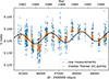 |
Fig. 1. S-index measurements of β Aql from the Mount Wilson HK-Project (blue circles) and the best-fitting sinusoid with a period of 4.7 yr and a linear slope (black curve). The orange points have been smoothed with a median filter that was 41 points wide. |
3. Observations
The observations we have used to perform asteroseismology on β Aql are described in the following sections. In addition to the data from SONG (Sect. 3.1) and TESS (Sect. 3.2), we have also analysed the RV measurements from SARG published by Corsaro et al. (2012, see Sect. 3.3) and unpublished archival RV measurements from HARPS (Sect. 3.4).
3.1. SONG (2022 and 2023)
In 2022 we observed β Aql with SONG-Tenerife over a period spanning 74 nights (11 July to 20 September 2022) with a median sampling cadence of 185 s. Observations were obtained on about two-thirds of these nights, with the coverage shown by the blue points in Fig. 2. We obtained data with SONG-Australia on 18 nights spread over 90 nights (23 June to 20 September 2022) during a period of very poor weather with a median sampling cadence of 250 s. These are shown by the orange points in Fig. 2. In 2023 we observed β Aql with SONG-Tenerife on 33 nights spread over 58 nights (20 June to 16 August 2023) with a median sampling cadence of 126 s.
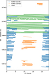 |
Fig. 2. Daily coverage of β Aql during the 2022 season from SONG and TESS. |
Radial velocities for both SONG nodes were extracted from the spectra using the pyodine software described by Heeren et al. (2023). The 2022 time series are shown in the top two panels of Fig. 3 and the 2023 time series from SONG-Tenerife is shown in Fig. 4. The processing of the time series is described in Sect. 4.
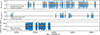 |
Fig. 3. Time series of β Aql from the 2022 season, showing radial velocities from SONG nodes in Tenerife (median uncertainty 3.0 ms−1) and Australia (median uncertainty 5.2 ms−1), and photometry from TESS (Sector 54; median uncertainty 68 ppm). Processing of the velocities and their uncertainties is described in Sect. 4. |
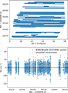 |
Fig. 4. Time series of β Aql from SONG Tenerife during the 2023 season. Top: nightly coverage of the measurements. Bottom: radial velocities (median uncertainty 2.3 ms−1; see Sects. 3.1 and 4). |
3.2. TESS (2022)
The Transiting Exoplanet Survey Satellite (TESS; Ricker et al. 2015) observed β Aql in Sector 54 (8 July to 5 August 2022). The light curve had a sampling cadence of 120 s and the temporal coverage is shown in Fig. 2 (green points). Given the brightness of the star, we extracted the light curve ourselves from the target pixel files using the lightkurve package (Lightkurve & Cardoso 2018). There are 17 900 measurements spanning 26.2 d and the processed time series is shown in the bottom panel of Fig. 3.
We note that Corsaro et al. (2024) analysed the TESS light curve of β Aql as part of a larger study of magnetically active solar-like oscillators. Using the standard PDCSAP light curve2, they reported νmax = 418 ± 4 μHz and Δν = 26.8 ± 1.9 μHz, which are consistent with our results (see Sect. 5.1).
After the analysis for this paper had largely been completed, a second sector of TESS data for β Aql became available (Sector 81). This sector does not overlap with the SONG observations presented in this paper so we have not included it, and we defer that analysis to a subsequent paper.
3.3. SARG (2009)
Solar-like oscillations were first detected in β Aql by Corsaro et al. (2012) using single-site observations with the SARG spectrograph at the Italian Telescopio Nazionale Galileo (TNG) 3.5 m telescope on La Palma. They observed over 6 nights in August 2009, using an iodine cell as the RV reference, and measured oscillations centred at νmax = 416 μHz (which corresponds to a period of 40 min). We have analysed those 809 RV measurements as part of this work (see Fig. 5). They have a median sampling of 192 s.
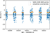 |
Fig. 5. Time series of RV measurements of β Aql from SARG in 2009 (median uncertainty 2.3 ms−1; see Sects. 3.3 and 4). |
3.4. HARPS (2008)
We retrieved 2200 unpublished RV measurements from the ESO archive that were obtained using the HARPS spectrograph (High Accuracy Radial velocity Planet Searcher) on the ESO 3.6m at La Silla in Chile. These measurements were taken on 17 nights spread over 35 nights in May and June 2008, with a median sampling cadence of 71 s. As shown in the top panel of Fig. 6, the observations on 8 nights spanned 4–5.5 h but the rest of the nights only contained 1–2 h of data. The processed time series (see Sect. 4 for details) is shown in the bottom panel of Fig. 6.
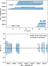 |
Fig. 6. Time series of β Aql from HARPS in 2008. Top: nightly coverage of the measurements. Bottom: radial velocities (median uncertainty 1.1 ms−1; see Secs. 3.4 and 4). |
4. Time-series processing
4.1. Introduction
Each of the time series described in Sect. 3 (SONG-Tenerife, SONG-Australia, TESS, SARG and HARPS) were processed separately using the steps described in the following sections (note that the SONG-Australia time series from the two 0.7-m telescopes were processed separately and then combined). Some of these steps involved applying a high-pass filter to the time series to remove slow trends by subtracting a smoothed version of the time series from the original:
 (1)
(1)
Note that the subscripts i and j in Equations (1)–(7) are indices of individual points in the time series. To create ysmoothed, we used a convolution in which each point was replaced by a weighted average of the points in its vicinity:
 (2)
(2)
where N is the total number of data points, and we chose the weighting function w to be a super-Lorentzian:
 (3)
(3)
The quantity Δt, which is the half-width at half-maximum of the weighting function, specifies the timescale of the high-pass filter. The values of Δt that we adopted are given in the next sections.
4.2. Removing bad data points
Each time series contains some bad data points that needed to be identified and removed. A small number of extreme outliers in the RV time series were removed by a simple clipping process (we used a threshold of ±20 ms−1, which removed 1.8% of the data points). We then identified less extreme outliers using the following procedure.
We first high-pass filtered the time series (see Sect. 4.1) but, in order to make this useful for identifying bad data points, we modified the smoothing process slightly. Instead of using Eq. (2), we created the smoothed version of the time series by replacing each data point by a weighted average of its neighbours excluding the point itself:
 (4)
(4)
In the weighting function (Eq. (3)) we set Δt to be the typical sampling time, calculated as the median value of (ti + 1 − ti). This small value of Δt means that the high-pass filtering only left the scatter on very short timescales.
The next step involved using this high-pass filtered time series, which we refer to as y1, to identify bad data points. We defined these bad points as having |y1|>5|y1,smoothed|, where |y1,smoothed| is the smoothed version of |y1| calculated based on Eq. (2) with a value of Δt = 0.05 d (1.2 h). The result of this process was an observed time series in which bad data points have been identified and removed. To illustrate the process, an example is shown in Fig. 7, where we have chosen a night with an unusually large number of bad points.
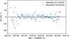 |
Fig. 7. One night of SONG-Tenerife data in 2022, illustrating bad data points that were discarded using the method outlined in Sect. 4.2. Note that this night had an unusually large number of bad points. |
4.3. Calculating uncertainties
The quality of the data varies during each time series and so it is very important to weight the data points when calculating the Fourier amplitude spectrum. For this we need to allocate an uncertainty σ(ti) to each data point y(ti). We did this using the time series y1 described in Sect. 4.2, recalculated with the bad data points removed. The smoothed uncertainties were then calculated as follows:
 (5)
(5)
which measures the scatter on short timescales. The calculation uses the weighting function wσ:
 (6)
(6)
and the half-width was once again Δt = 0.05 d (1.2 h). We used the exponent of 8 instead of 4 to make the function even more box-like, to give less sensitivity to points that were not close to the point under consideration. In some cases, a small segment of the time series was given too much weight because it had very low scatter. To avoid this, we set a lower limit on σ(ti) of 0.7 times the median value.
Before calculating the Fourier amplitude spectrum of the time series, we applied a high-pass filter (Eqs. 1–3) with Δt = 0.05 d (1.2 h). These time series are shown as blue points in Figs. 3 to 5. The amplitude spectrum was then calculated using σ(ti)−2 as weights (see Frandsen et al. 1995) and the results are discussed in the next section. Finally, we rescaled σ(ti) to reflect the mean noise in the weighted amplitude spectrum, σamp, as measured at high frequencies. That is, we multiplied the uncertainties by a constant so that they satisfied equation (3) of Butler et al. (2004):
 (7)
(7)
We repeated the steps in Sections 4.2 and 4.3 until no additional data points were removed. The total number of data points removed in each time series was 2–3%. The final uncertainties are shown as orange points in Figs. 3 to 5 and the median values are given in the figure captions. We would be happy to provide these time series of measurements and uncertainties upon request.
5. Analysis of oscillations
5.1. Weighted power spectra
The weighted power spectra of the five time series discussed above are shown in Fig. 8. The oscillations are clearly detected in all data sets, and the TESS data also show rising power towards low frequencies arising from surface granulation. As mentioned in the Introduction, the granulation background is much lower (relative to the oscillations) in RV measurements. For each power spectrum we indicate νmax and the amplitude per radial mode, which we measured using the method described by Kjeldsen et al. (2008a). In summary, this involves heavily smoothing the power spectrum, converting to power density, fitting and subtracting the background from white noise and granulation, and multiplying by c/Δν, where c is the effective number of modes per order (normalized to ℓ = 0). We used Δν = 27.3 μHz (see Sec 5.5), and chose c = 4.09 for the RV measurements and c = 2.95 for the TESS photometry (see Kjeldsen et al. 2008a for more details).
 |
Fig. 8. Power spectra of β Aql showing solar-like oscillations from four time series in radial velocity and one in TESS photometry, with measurements of νmax and amplitude per radial mode (see Sect. 5.1). The bottom panel shows the reconstructed power spectrum from the combined SONG and TESS data, smoothed to a resolution of 1 μHz (see Sect. 5.5). |
The values of νmax show some scatter between the different data sets, which presumably reflects fluctuations arising from the stochastic nature of the excitation and damping. On the other hand, some of the scatter could reflect variations between the different observing techniques. There is perhaps some indication that the RV amplitude has changed during the 14 years spanned by the observations, which might be expected if the star has a magnetic activity cycle (see Sect. 5.7 for further discussion).
These data sets give an excellent opportunity to compare measurements of oscillations in velocity and photometry, especially since they were obtained simultaneously. The best previous example of such a comparison comes from the Sun and we discuss solar measurements in the next section, before returning to β Aql in Sect. 5.3.
5.2. The solar oscillations in photometry and velocity
We briefly digress to discuss the amplitude of oscillations in the Sun. In photometry, the best available intensity measurements come from the VIRGO instrument (Variability of solar IRradiance and Gravity Oscillations) on the SOHO spacecraft (Solar & Heliospheric Observatory), which has been operating since 1996 (Fröhlich et al. 1995, 1997). VIRGO provides photometric time series in three channels: blue (402 nm), green (500 nm) and red (862.5 nm). We have measured the solar amplitude over the full data set by applying the method described in Sect. 5.1 to 25-day non-overlapping segments of the time series. The results are shown in Fig. 9.
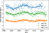 |
Fig. 9. Peak amplitude of the solar oscillations measured over 27 years using data from the three-channel solar photometers (SPM) on the VIRGO Experiment aboard the SOHO spacecraft. Points are measurements from 25-day non-overlapping segments of the time series and the solid curves result from a median filter followed by smoothing with a Gaussian window (FWHM = 1 yr). The lack of points in the 400-nm data towards the end of the series is a result of reduced data quality, with too few points for reliable amplitude measurements. |
It is clear from Fig. 9 that the photometric amplitude of the solar oscillations varies over the Sun’s 11-year activity (see also Jiménez-Reyes et al. 2003; Kim & Chang 2022) and the same behaviour is seen in velocity amplitudes (Chaplin et al. 2000, 2003; Kjeldsen et al. 2008a; Kiefer et al. 2018; Howe et al. 2022). We also see that the photometric amplitude depends on wavelength, which is a well-known phenomenon for solar-like oscillations (e.g. Kjeldsen & Bedding 1995; Ballot et al. 2011; Lund 2019; Sreenivas et al. 2025). In order to compare photometric amplitudes from different instruments (and also to compare photometry with velocity), it is convenient to consider the bolometric amplitude of an oscillating star. This is the fractional variation in amplitude that would be measured if the observations covered all wavelengths. The notation for this quantity used by Kjeldsen & Bedding (1995) was (δL/L)bol but here we adopt the more compact notation of Abol (e.g. Lund 2019). As noted by Kjeldsen & Bedding (1995), this is related to the amplitude at a given wavelength by the approximate relation
 (8)
(8)
Here,
 (9)
(9)
is the wavelength at which the observed luminosity amplitude (Aλ) is equal to Abol. A more accurate version of Eq. (8) was derived by O’Toole et al. (2003)3. Assuming the luminosity changes come entirely from changes in temperature (so that changes in stellar radius can be neglected), the relation is
 (10)
(10)
We used Eq. (10) to estimate the bolometric amplitude of the Sun from our time series of VIRGO measurements. We took the weighted mean of the green and red channels, since these fall on either side of the bolometric wavelength of the Sun, which is λbol, ⊙ = 623 nm. We averaged the measurements over two solar cycles (22 yrs) to get
 (11)
(11)
This is slightly lower than the values previously measured from VIRGO data, namely 3.58 ± 0.16 ppm obtained by Michel et al. (2009)4 and 3.5 ± 0.2 ppm obtained by Huber et al. (2011a). Given that the value in Eq. (11) has been averaged over two full solar cycles, we consider it to be the most reliable.
We now turn to the velocity amplitude of the solar oscillations. Here, we are interested in observations made using stellar techniques, which involve measuring the radial velocity from a wide wavelength range that includes a large number of spectral lines. As discussed in detail by Kjeldsen et al. (2008a), these give different amplitudes to the single-line RVs measured by dedicated helioseismology instruments such as BiSON and GOLF. The longest solar data using stellar techniques was measured with SONG-Tenerife over 57 consecutive days in mid-2018 by Andersen et al. (2019). They reported the average amplitude of the strongest radial modes as vosc, ⊙ = 0.166 ± 0.004 ms−1 (measured using the same method as in this paper—see Sect. 5.1). We can adjust for the fact that the VIRGO amplitude during those observations was 3.3 per cent higher than the average over two activity cycles, which then gives the mean solar amplitude in velocity to be
 (12)
(12)
To conclude, Eqs. 11 and 12 give our best estimates for the mean oscillation amplitude in the Sun in photometry and velocity.
5.3. Photometry-to-velocity amplitude ratio of β Aql
β Aql now joins a small number of stars for which solar-like oscillations have been observed in both RV and photometry, and an even smaller number for which these observations were simultaneous (Procyon is the only published example of which we are aware; see Huber et al. 2011b). This allows us to measure the ratio between the two types of measurements (see also Houdek 2010; Arentoft et al. 2019; Zhou et al. 2021).
Note that simultaneous measurements are highly preferable for this purpose because of the large variations in amplitude that are intrinsic to solar-like oscillations. We measured the RV amplitude in the part of the SONG time series that overlapped with the TESS data (see Fig. 2) to be vosc = 0.497 ± 0.044 ms−1. Meanwhile, the TESS photometric amplitude was 11.9 ± 0.9 ppm (Fig. 8). Because TESS has a very broad passband, we did not use Eq. (10). Instead, we converted the TESS amplitude to the bolometric amplitude by multiplying by cT − bol = 1.066 ± 0.011, which we calculated from Eq. (7) of Lund (2019) using Teff = 5092 ± 50 K. This gave the photometric amplitude of β Aql as Abol = 12.7 ± 1.0 ppm.
The photometry-to-velocity ratio for β Aql is therefore
 (13)
(13)
The same ratio for the Sun, using Eqs. (11) and (12), is
 (14)
(14)
According to Kjeldsen & Bedding (1995), this ratio is expected to scale inversely with Teff. The effective temperatures of the Sun and β Aql are in the ratio 1.134 ± 0.011, whereas the values in Eqs. (13) and (14) are in the ratio 1.36 ± 0.17. These values agree within the uncertainties (1.3σ), although it would clearly be desirable to improve the accuracy for β Aql.
We have also examined the photometry-to-velocity ratio as a function of frequency, as shown in the upper panel of Fig. 10. This plot was created by dividing a heavily smoothed version of the TESS power spectrum by a similarly smoothed version of the SONG power spectrum (using all data) and then taking the square root. For both TESS and SONG, we first removed the background by fitting components for white noise and granulation (where the latter used a simple Harvey profile; see Harvey 1988). The smoothing was achieved by convolving with a Gaussian having a FWHM of 4Δν. We see a strong trend in the ratio as a function of frequency which does not appear to agree with theoretical expectations (Houdek 2010) and clearly deserves further study. The granulation background, which is stronger in TESS data, has been subtracted before calculating the amplitude ratio but we note that incorrect subtraction would lead to trends at in amplitude at low frequencies. For this reason, we restricted the plot in Fig. 10 to frequencies above 270 μHz, where the granulation background is very low. As a further check on this result, we also calculated the ratio between the two sets of SONG RV data. As shown in the lower panel of Fig. 10, this ratio is independent of frequency but shows a possible increase in the oscillation amplitude from 2022 to 2023 (see Sect. 5.7).
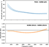 |
Fig. 10. Ratio between amplitude spectra obtained with TESS and SONG (upper panel) and between the two seasons of SONG data (lower panel), smoothed to 4Δν (see Sect. 5.3). |
Regarding the increase in the photometry-to-velocity ratio towards lower frequencies, we note that a similar trend was reported in the Sun by Jiménez (2002). By analysing the heights of individual modes as measured by VIRGO and GOLF, they found the amplitude ratio at 2 mHz to be higher by a factor of two higher than at 3–4 mHz (see Figure 6 in that paper). Magnetic activity probably affects amplitudes and phases, which theoretical models do not include. We note that the value of νmax would also be affected, causing it to be lower when measured in photometry than in velocity. Indeed, this effect may be be partially responsible for such a finding in the K0 dwarf σ Dra by Hon et al. (2024), using photometry from TESS and radial velocities from the Keck Planet Finder (KPF).
5.4. Comparing the simultaneous intensity and velocity signals
Since a small part of the SONG data overlaps in time with TESS, we can directly compare the signals in intensity and velocity. To do this, we isolated the oscillation signal in each time series using a band-pass filter. This was implemented by using the standard method of iterative sine-wave fitting (see also Sect. 5.5) to extract 10,000 sinusoidal components in the frequency range 330–550 μHz, which covers the region in which we see excess power from oscillations. We then reconstructed the time series as the sum sinusoids using these extracted frequencies, amplitudes and phases.
Figure 11 shows the results for the 8 nights on which SONG was observing simultaneously with TESS. We see a clear indication of a phase shift between the SONG and TESS data. The signal-to-noise and the length of the time series are not high enough to measure the phase shifts for individual oscillation modes, so we estimated the phase shift for the combined oscillation signal. We initially did this by calculating the cross correlation between the TESS and SONG data for each of the segments separately. This gave a shift in time between the two series for each segment, which we converted to a phase shift using the typical timescale of the oscillations (measured from the peak of the cross-correlation function for that segment). Only five of the segments were long enough to provide a robust measurement, and we calculated the average phase shift to be −151° ±25° = − 2.64 ± 0.44 rad.
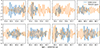 |
Fig. 11. Observations of β Aql on eight nights that had overlap between SONG and TESS. Each panel shows a 10-h segment, with radial velocities from SONG-Tenerife in ms−1 (blue curves) and TESS photometry divided by 25 ppm (orange curves). Both series have been bandpass-filtered to show variations in the range 330–550 μHz. |
As well as treating the overlapping segments separately, we also calculated the cross correlation using the entire section for which there was overlap. This gave better accuracy and we calculated the phase shift to be −113° ±7°. In other words, the peak of the SONG oscillations (highest positive RV) occurs 31 per cent of an oscillation period before the peak of the TESS signal.
In the Sun, the corresponding phase shift can be measured using SOHO observations (Jiménez 2002). We used one month of data from GOLF and VIRGO to measure the phase shift in the Sun to be −125.6° ±0.5°. This is close to the β Aql value but differs by 1.8σ (although we do not necessarily expect exact agreement) and a longer overlapping time series for β Aql is needed to give a more precise measurement. We also note that in the Sun, Jiménez (2002) found the phase difference between velocity and intensity to vary by as much as 10 degrees over the solar activity cycle (their Figure 4). They also noted that the effects of changing magnetic activity are not included in the models by Houdek et al. (1995).
Importantly, these results indicate that high-cadence photometric observations with TESS could be used to infer the corresponding velocity oscillation signal, and hence to improve the precision of simultaneous RV measurements. This is highly relevant to high-precision RV searches for exoplanets (e.g. Dumusque et al. 2011; Yu et al. 2018; Chaplin et al. 2019; Nieto & Díaz 2023; Zhao et al. 2023; Luhn et al. 2023; Gupta & Bedell 2024; O’Sullivan & Aigrain 2024; Zhao et al. 2024; Beard et al. 2025; Tang et al. 2025).
It is also interesting to compare our measured phase difference with 3D hydrodynamical simulations of stellar atmospheres. As a preliminary comparison, we have used a simulation that was previously computed using the STAGGER code for a star with Teff = 5000 K and log g = 3.5 (Magic et al. 2013). These values are similar to those of β Aql (Teff = 5092 K and log g = 3.55). The simulated time series consists of 3000 snapshots with a sampling cadence of 166 s and a total duration of 138.33 hours of stellar time. We measured the phase difference between the stellar flux variations and the vertical fluid velocity to be −121° ±6°, which is in excellent agreement with our measurements for β Aql.
5.5. Extraction of mode frequencies
To extract frequencies of the oscillation modes, we first generated a reconstructed power spectrum based on the data from SONG (2022), SONG (2023) and TESS. The SONG data, in particular, are affected by gaps in the time series that introduce sidelobes in the power spectra. The first step was to reconstruct power spectra for each data set using the standard method of iterative sine-wave fitting (also called prewhitening), using the uncertainties as weights. For each of these three data sets, we extracted 10 000 sinusoidal components in the frequency range 200–700 μHz to ensure that all power–including the noise–was included. We then created a reconstructed power spectrum as the sum of δ functions with those frequencies and heights.
Having done this, we corrected the TESS spectrum for the granulation background, which rises towards lower frequencies. We did this by fitting and dividing by a function of the form (ν/νmax)−2, which matches the slope of the granulation background (e.g. Sreenivas et al. 2024). Since SONG and TESS observe different quantities, we normalized each reconstructed power spectrum to have a mean of 1 before averaging them. This final reconstructed power spectrum was smoothed by convolving with a Gaussian with a FWHM of 1 μHz, chosen to match approximately the lifetime of the modes. The reconstructed spectrum is shown in the bottom panel of Fig. 8.
The reconstructed spectrum is shown in échelle format in Fig. 12, where the power spectrum has been divided into equal segments of width Δν that are stacked vertically. The value of Δν = 27.3 μHz was chosen to make the ridges vertical. This échelle diagram reveals a pattern typical of a star in this evolutionary state, with a clear vertical ridge corresponding to modes with ℓ = 0, accompanied by a weaker ridge to its left (ℓ = 2 modes) and several other peaks that are spread over the rest of the diagram (mixed ℓ = 1 modes). Very similar patterns have been seen in late subgiants and early red giant branch (RGB) stars observed by Kepler, particularly in KIC 4351319 (nicknamed ‘Pooh’; di Mauro et al. 2011) and KIC 7341231 (‘Otto’; Deheuvels et al. 2012).
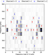 |
Fig. 12. Power spectrum of β Aql reconstructed from the SONG and TESS data, shown in échelle format. The greyscale shows the reconstructed power spectrum (Sect. 5.5) and the open blue symbols show the identified modes, while red crosses are assumed to be noise peaks (see Table 1). |
We extracted oscillation mode frequencies from the reconstructed power spectrum by measuring the strongest peaks in the frequency range 300–550 μHz, which is the region that contains the oscillations. The 40 strongest peaks are listed in Table 1. There is always a risk that the pre-whitening could latch on to a sidelobe, and so we must keep in mind that some modes maybe be off by one cycle per day (±11.57 μHz). As a check, we applied the Gold deconvolution algorithm (Morháč et al. 2003; Li et al. 2025) and found very similar results.
In order to estimate uncertainties on the frequencies, we ran a number of simulations for modes with a lifetime similar to the Sun. We generated time series with the same length as the data and smoothed the power spectra to a resolution of 1 μHz before measuring the peak positions. We ran simulations at different SNR to estimate the error bars for the individual extracted modes (see De Ridder et al. 2006).
The mode identifications are listed in Table 1. We identified 6 radial modes (ℓ = 0) and 3 quadrupolar modes (ℓ = 2) based on their positions in the échelle diagram (Fig. 12). We also identified 13 mixed ℓ = 1 modes, using the method described in the next section. Finally, 18 peaks in Table 1 that were not identified as modes are presumably noise peaks (red crosses Fig. 12).
We note that the radial velocity of β Aql is vr = −41.50 ± 0.68 kms−1 (Steinmetz et al. 2020), which means that the oscillation frequencies have been Doppler shifted by a factor of (1 + vr/c), where c is the speed of light. The observed frequencies should be multiplied by this factor before carrying out detailed modelling (Davies et al. 2014), which amounts to a shift of 0.047–0.065 μHz over the range of detected modes. We show the uncorrected frequencies in Table 1 but made the Doppler correction before carrying out the modelling described in Sect. 6.
5.6. Identifying mixed modes
While it is straightforward to identify ℓ = 0 and 2 modes using the échelle diagram (Fig. 12), it is more difficult to decide which of the remaining peaks represent ℓ = 1 modes and which are noise peaks. To do this, we took advantage of the fact that ℓ = 1 mixed modes follow a definite pattern. They result from coupling of pure p modes and pure g modes, both of which are in the asymptotic regime. This means pure p modes with radial order np are approximately equally spaced in frequency by Δν, with νp ≈ Δν(np + ϵp, ℓ = 1). Here, ϵp, ℓ = 1 is the p-mode phase term. Similarly, pure g modes are approximately equally spaced in period by ΔΠ1, with 1/νg ≈ ΔΠ1(ng + ϵg), where ng is the radial order of each g mode and ϵg is the g-mode phase term.
Initial modelling based on the ℓ = 0 and ℓ = 2 modes (see Sect. 6 for a full description of the models) found good agreement with a model with a period spacing of ΔΠ1 = 108.7 s. We used this value to construct a so-called stretched period échelle diagram for the power spectrum, by converting frequency ν to stretched period τ, which is defined as follows (Mosser et al. 2015; Ong & Gehan 2023):
![Mathematical equation: $$ \begin{aligned} \tau = \frac{1}{\nu } + \frac{\Delta \Pi _1}{\pi } \arctan \left[ \frac{q}{\tan (\nu /\Delta \nu - \epsilon _{p,\ \ell =1})} \right]. \end{aligned} $$](/articles/aa/full_html/2025/08/aa54633-25/aa54633-25-eq17.gif) (15)
(15)
The dipole (ℓ = 1) mixed modes will align vertically in the stretched period échelle diagram, provided the asymptotic parameters appearing in the equation (the phase term ϵp and the coupling strength q) are appropriately chosen. By iteratively optimizing these parameters, we found that values of ϵp, ℓ = 1 = 1.95 and q = 0.25 produced the best alignment, with the l = 1 modes (blue triangles) reasonably close to the vertical dashed line in Fig. 13. The position of that vertical alignment indicates that the pure-g modes are asymptotically spaced, with a phase of ϵg = 0.52. Based on their proximity to this line we identified 13 ℓ = 1 mixed modes, as listed in Table 1.
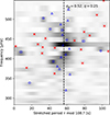 |
Fig. 13. Stretched period échelle diagram, as described in Sect. 5.6. The greyscale shows the reconstructed power spectrum, and the symbols showing identified modes (blue) and noise peaks (red crosses) have the same meanings as in Fig. 12. |
5.7. Amplitude and frequency variations from 2022 to 2023
Given that β Aql appears to undergo a magnetic activity cycle with a period of 4.7 ± 0.4 yr (Fig. 1), we might expect to see changes in the amplitudes and frequencies of its oscillation modes. Such changes are well documented in the Sun (see review by Chaplin et al. 2014) and have also been seen in other stars (e.g. García et al. 2010; Kiefer et al. 2017; Salabert et al. 2018; Santos et al. 2018). With SONG we see an increase in oscillation amplitude from 2022 to 2023 of 25%±8%, which is a 3-σ change (see Figs. 8 and 10). By comparison, the intrinsic variation of the oscillation amplitudes in the Sun over the solar cycle is 10% peak-to-peak (Kjeldsen et al. 2008a). Continued SONG observations of β Aql over the coming years should help to clarify whether these changes are related to its activity cycle.
We also compared the frequencies of individual modes in the SONG 2022 and 2023 data. The mean frequency difference is 0.019 ± 0.082 μHz (a fractional change of (0.4 ± 1.9)×10−4), which is a non-detection. The peak-to-peak shift in the solar frequencies over the full activity cycle is about 0.4 μHz (a fractional change of 1.3 × 10⁻⁴ (Jimenez-Reyes et al. 1998; Chaplin et al. 2007, 2014). Therefore, our current upper limit on frequency shifts in β Aql–when expressed as a fractional change–is greater than that seen in the Sun.
6. Asteroseismic Modelling
6.1. Modelling methods
To perform asteroseismic model fitting, we constructed theoretical stellar models using MESA (version r23.01.1; Paxton et al. 2011, 2013, 2015, 2018, 2019; Jermyn et al. 2023) and GYRE (version 7.0; Townsend & Teitler 2013). We used pp_and_cno_extras for nuclear reaction rates (Cyburt et al. 2010; Angulo et al. 1999). The metallicity scale and metal mixture were chosen to be the AGSS09 solar abundance scale (Asplund et al. 2009). Compatible opacity tables were used (‘a09’, ‘lowT_fa05_a09p’, and ‘a09_co’; Iglesias & Rogers 1996; Ferguson et al. 2005). The mixing-length theory was used for treating convection following the formalism of Henyey et al. (1964). The grey Eddington T–τ relation was used as the atmospheric boundary condition (Eddington 1926). We did not include any mass loss, diffusion, overshoot, or other non-standard mixing processes. In particular, we note that the extent of core overshooting is small at 1.2M⊙ (Claret & Torres 2018; Lindsay et al. 2024). All other settings adhered to MESA defaults. Our MESA inlists are available at this URL5.
Properties of β Aql.
The stellar model grid was sampled uniformly in a four-dimensional parameter space. The stellar mass ranged from 1.0 to 1.4 M⊙ with a step size of 0.02 M⊙; the mixing length parameter αMLT ranged from 1.5 to 2.7 with a step size of 0.2 (which comfortably includes the expected range; see Sect. 6.2); the initial helium abundance Yinit ranged from 0.18 to 0.34 with a step size of 0.02; and the metallicity [M/H] ranged from −0.65 to 0.05 dex with a step size of 0.05 dex. All tracks were evolved until Δν dropped below 22 μHz on the red giant branch. Stellar oscillation modes were calculated using GYRE on-the-fly (Bellinger 2022); Joyce++2024 for models that fell within a 5-σ constraint box specified by Teff, R, and [M/H].
To evaluate each model in the grid, we constructed a χ2 function incorporating both the classical observables of β Aql (c = {R, Teff, [Fe/H]}; Table 2) and the oscillation frequencies (ν = {νk; k = 1, …Nl, l = 0, 1, 2}; Table 1). The χ2 function was defined as
 (16)
(16)
where the subscripts “obs” and “mod” indicate observational and modelling quantities, respectively, and the σ values are the observational uncertainties. For each model i, the posterior probability was computed as pi ∝ Δtiℒi = Δtiexp(−χi2/2), where Δti is the time-step between adjacent models on the evolutionary track to account for numerical unevenness in the spacing. Each stellar parameter θi was estimated from the cumulative distribution of pi(θi), with the 50% percentile representing the best-fitting value and the 16% and 84% percentiles providing the 1-σ confidence intervals.
It is well established that model frequencies need to be corrected for inaccurate treatment of the near-surface layers (e.g. Christensen-Dalsgaard et al. 1996; Kjeldsen et al. 2008b; Ball & Gizon 2014; Jørgensen et al. 2020; Belkacem et al. 2021; Ong et al. 2021; Li et al. 2023a). In this work, we parametrized the surface correction using the cubic formula proposed by Ball & Gizon (2014). This formula can yield inaccurate results for mixed modes in red giants (Ball et al. 2018; Li et al. 2018), but studies by Ong et al. (2021) demonstrated its suitability for early subgiants such as β Aql, which have high coupling strengths.
Figure 14 shows the differences, scaled by mode inertia, between observed frequencies and those of the best-fitting model (before making the surface correction). We see that these scaled differences follow the cubic formulation within statistical uncertainties. Further, to avoid the surface correction from become unphysically large or small, we constrained it to vary smoothly as a function of stellar parameters (e.g. Compton et al. 2018; Li et al. 2023a; Reyes et al. 2025a). This was done by setting the amount of surface correction at νmax to be 4.5% of Δν, which we determined based on the best-fitting model when we treated surface correction with free parameters, as originally proposed by Ball & Gizon (2014). We note that this amount of surface correction is in agreement with that expected from the ensemble study by Li et al. (2023a, their Equation 4 and Table 2).
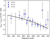 |
Fig. 14. Differences, scaled by mode inertia, between the observed frequencies and those of the best-fitting model (before making the surface correction). The differences approximately follow the cubic formula proposed by Ball & Gizon (2014), as shown by the solid line. |
6.2. Stellar parameters
Figure 15 shows the position of β Aql in the Hertzsprung–Russell diagram, as well as the grid of theoretical models, confirming that the star is at the base of the red giant branch. The frequencies of the best-fitting model are shown in Fig. 16 (filled grey symbols), and we see an excellent match with most of the observed frequencies (open blue symbols). In Table 2 we list the stellar parameters, including mass, age, log g, mean density, αMLT, and Yinit. We note that the uncertainties of log g and density are probably underestimated, since the systematic uncertainties can be many times larger than the statistical uncertainties reported here (e.g. Huber et al. 2022).
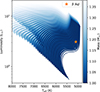 |
Fig. 15. Hertzsprung–Russell diagram showing the observed location of β Aql and the grid of theoretical models (see Sect. 6). |
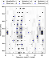 |
Fig. 16. Reconstructed power spectrum of β Aql (greyscale) with the observed frequencies (open blue symbols; Table 1) and model frequencies (filled black symbols). For the latter, the symbol sizes for the non-radial modes are inversely proportional to mode inertia, scaled to the inertia of adjacent radial modes. |
There has been considerable discussion about whether the choice of weighting terms appearing in Equation 16 (such as 1/Nl) can affect the derived stellar parameters (e.g. Cunha et al. 2021). To investigate this, we tested an alternative approach where 1/Nl was replaced with a value of 1, effectively treating each mode frequency as equally important as each classical observable. This adjustment resulted in no statistically significant changes in the estimated mass and age, showing the robustness of these derived stellar parameters against the choice of weighting scheme.
We determined a mass of 1.24 ± 0.02 M⊙. Recent studies using only classical observables have reported less precise results. For example, Ghezzi & Johnson (2015) reported 1.140 ± 0.105 M⊙ with PARSEC models (Bressan et al. 2012), and Karovicova et al. (2022) obtained 1.36 ± 0.13 M⊙ with Dartmouth stellar evolution tracks (Dotter et al. 2008). These comparisons demonstrate the significant improvement in precision when asteroseismic data are incorporated. However, we caution that the reported precision is not entirely realistic for several reasons: (i) the observational frequency uncertainties are often very small, which disproportionately dominates the likelihood function compared to the classical constraints (Cunha et al. 2021; ii) the model uncertainties in the frequencies typically dominate, yet they are difficult to quantify when relying on a single set of models with limited variations in input physics (Silva Aguirre et al. 2020; Christensen-Dalsgaard et al. 2020; Li et al. 2024); and (iii) the model-predicted frequencies are often correlated, but these correlations are rarely incorporated into the analysis (Aerts et al. 2008; Li et al. 2023b).
The value of νmax implied by our model fits is 423 ± 5 μHz, based on the standard scaling relation of  (Brown et al. 1991; Kjeldsen & Bedding 1995), which falls within the range of measured values (see Fig. 8). We also note that we used the measured interferometric radius of β Aql as an input to the modelling. If this measurement is not used, the stellar mass and radius agree with those listed in Table 2 but with uncertainties increased by about a factor of two.
Our asteroseismic analysis gives the age of β Aql to be 4.77 ± 0.50 Gyr, which again is consistent with classically determined stellar ages but more precise. For example, an age of 5.86 ± 1.87 Gyr was reported by Ghezzi & Johnson (2015). We note that our result also gives an accurate age for the M-dwarf companion, β Aql B (see Sect. 2).
Including the interferometric radius in the fit has allowed us to constrain the mixing-length parameter quite well. At the base of the RGB, determining the radius with asteroseismology using individual frequencies alone (without νmax) is challenging due to the strong correlation between the radius and αMLT (Li et al. 2024). An accurate angular diameter makes β Aql an important calibrator for αMLT in this region of parameter space. We determined αMLT for β Aql to be 2.10 ± 0.15. The uncertainty is comparable to the grid step size, which suggests that the precision could be further improved by using finer sampling in the αMLT parameter space. Hydrodynamical 3D simulations suggest that stars with properties similar to β Aql should have values similar to that of the Sun (Trampedach et al. 2014; Magic et al. 2015). In fact, our value for β Aql is slightly higher than our solar-calibrated value of 1.9, and a similar difference between 1D modelling and 3D simulations has been reported from analysis of Kepler stars (Tayar et al. 2017; Viani et al. 2018; Li et al. 2018; Joyce & Tayar 2023).
Models that excluded mixed-mode frequencies failed to constrain the initial helium abundance (Yinit). However, when mixed-mode information was included, Yinit became better constrained. We found that using the g-mode period spacing alone was insufficient to achieve this constraint. Instead, the improvement is attributed to the g-mode phase (ϵg), presumably through the modulation of the location of the g-mode cavity from chemical abundances. This aspect clearly warrants further detailed investigation.
6.3. Comparison with M67
β Aql is in a similar evolutionary state to some members of the solar-metallicity open cluster M67, for which Reyes et al. (2024) recently determined an age of  Gyr. Using photometry from Kepler/K2, Reyes et al. (2025a) have detected oscillations in more than 30 subgiants and RGB stars in M67, and we have compared them with our results for β Aql, and a representative stellar track of a 1.22 M⊙, [Fe/H]= − 0.21 star, created and surface-corrected as described in that paper.
Figure 17 shows the comparison on two important asteroseismic diagrams. The upper panel shows the so-called C-D diagram (Christensen-Dalsgaard 1988), which plots the small separation versus the large separation. The small frequency separation, δν02, is the mean difference between modes of degrees ℓ = 0 and 2, which we measured for β Aql by vertically collapsing the échelle diagram and fitting Lorentzian functions to the two ridges (e.g. Bedding et al. 2010). This method boosts the signal-to-noise ratio of ℓ = 0 and ℓ = 2 modes while also reducing the impact of mixed modes on the final δν02 measurements. The lower panel plots Δν against the phase term, ϵ, which measures the absolute position of the mode pattern found from the above fit of the radial ridge (Christensen-Dalsgaard 1988; Huber et al. 2010; White et al. 2011a,b; Kallinger et al. 2012; Christensen-Dalsgaard et al. 2014), as shown by the asymptotic relation for acoustic modes (Tassoul 1980):
 (17)
(17)
where νnℓ is the frequency of the mode of radial order n and degree ℓ.
The seismic properties of β Aql align remarkably well with the sequence observed in M67, despite the difference in metallicity ([Fe/H] for M67 is close to zero). The wiggles seen in the C–D diagram depend on the location of the bottom of the convection zone, which in turn depends on mass and metallicity (Reyes et al. 2025b). Because β Aql is slightly lower in both metallicity and mass than the M67 giants, it still falls close to the M67 sequence in the diagram. The star’s location in this particular region of the diagram would suggest it is well suited to investigate the amount of overshooting at the bottom of the convective envelope (Ong et al. 2025; Reyes et al. 2025b). However, at the evolutionary stage of β Aql we expect some scatter in the observed δν02 values due to mixed modes. This results in β Aql effectively blending in with the M67 sequence. At the evolution stage, metallicity, and mass of β Aql, the ϵ diagram is not expected to show clear sensitivity to metallicity and mass (White et al. 2011a), which is confirmed by the alignment with the M67 sequence.
7. Conclusions
We have presented time-series radial velocities of the G8 subgiant star β Aql obtained in 2022 and 2023 using SONG-Tenerife and SONG-Australia. We describe our method for processing the time series to assign weights to the observations and remove bad data points. The resulting power spectrum clearly shows solar-like oscillations, and these are also seen in the power spectra of the 2022 TESS light curve and of short RV time series obtained with HARPS (in 2008) and SARG (in 2009).
β Aql is only the second star, after Procyon, for which we have observations of solar-like oscillations simultaneously in RV and photometry. We measured the ratio between the bolometric photometric amplitude and the velocity amplitude to be 26.6 ± 3.1 ppm/ms−1 (Sect. 5.3), which compares with our measurement for the Sun (made using published data from SOHO/VIRGO and SONG-Tenerife) of 19.5 ± 0.7 ppm/ms−1 (Sect. 5.2). Once the difference in effective temperatures of the two stars is taken into account, these measurements agree within their uncertainties. We also measured the phase shift of the oscillations between SONG RVs and TESS photometry to be −113° ±7°, which agrees within uncertainties with the value in the Sun and with a 3D simulation (Sect. 5.4). Importantly, these results indicate that high-cadence photometric observations with TESS could be used to mitigate the effect of oscillations on RV exoplanets searches.
We extracted frequencies for 22 oscillation modes with angular degrees of ℓ = 0, 1 and 2 (Table 1). We carried out asteroseismic modelling by comparing the observed properties of β Aql with a grid of models, yielding an excellent fit to the frequencies. The resulting stellar parameters are listed in Table 2. In particular, we have been able to place quite strong constrains on the mixing length parameter (αMLT) by including the interferometric radius in the model fitting. We also found that the oscillation properties of β Aql are very similar to subgiants and low-luminosity RGB stars in the open cluster M67 (Fig. 17). Further observations of β Aql with SONG will be valuable, especially since the Mount Wilson S-index measurements show evidence of a magnetic activity cycle with a period of 4.7 yr (Sect. 2).
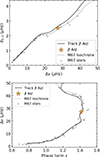 |
Fig. 17. Small frequency separations δ0, 2 (top) and phase term ϵ (bottom) sequences from M67 stars, taken from Reyes et al. 2025b and Reyes et al. 2025a, respectively. β Aql is shown with a star symbol. |
Pre-search Data Conditioning Simple Aperture Photometry, available from the Mikulski Archive for Space Telescopes, https://archive.stsci.edu/.
Note Eq. (5) of O’Toole et al. (2003) is missing a factor of 4 in the denominator. The correct version is given in Eq. (9) above.
Michel et al. (2009) measured 2.53 ± 0.11 ppm, but this was the rms amplitude and needs to be multiplied by  .
.
Acknowledgments
The SONG network of telescopes is operated by Aarhus University, Instituto de Astrofísica de Canarias, the National Astronomical Observatories of China, University of Southern Queensland and New Mexico State University. We are grateful to the observing and technical support at each of the sites. We especially acknowledge Antonio Pimienta for his role as the curator of the Hertzsprung SONG Telescope at the Observatorio del Teide continuously for the past 15 years. Funding for the Stellar Astrophysics Centre was provided by The Danish National Research Foundation (Grant agreement no.: DNRF106). We gratefully acknowledge support from the Australian Research Council through: LIEF Grant LE190100036; Discovery Projects DP220102254 (SLM) and DP210101299 (JL); Future Fellowships FT210100485 (SJM) and FT200100871 (DH); and Laureate Fellowship FL220100117 (TRB). PLP acknowledges support from the Spanish Ministry of Science and Innovation with the grant no. PID2023-146453NB-100 (PLAtoSOnG). The HK_Project_v1995_NSO data derive from the Mount Wilson Observatory HK Project, which was supported by both public and private funds through the Carnegie Observatories, the Mount Wilson Institute, and the Harvard-Smithsonian Center for Astrophysics starting in 1966 and continuing for over 36 years. These data are the result of the dedicated work of O. Wilson, A. Vaughan, G. Preston, D. Duncan, S. Baliunas, and many others. SOHO is a project of international cooperation between ESA and NASA. This work made use of several publicly available python packages: astropy (Astropy Collaboration 2013, 2018), echelle (Hey & Ball 2020), lightkurve (Lightkurve & Cardoso 2018), matplotlib (Hunter 2007), numpy (Harris et al. 2020), and scipy (Virtanen et al. 2020).
References
- Addison, B., Wright, D. J., Wittenmyer, R. A., et al. 2019, PASP, 131, 115003 [NASA ADS] [CrossRef] [Google Scholar]
- Aerts, C., Christensen-Dalsgaard, J., Cunha, M., & Kurtz, D. W. 2008, Sol. Phys., 251, 3 [Google Scholar]
- Aerts, C., Christensen-Dalsgaard, J., & Kurtz, D. W. 2010, Asteroseismology (Springer) [Google Scholar]
- Andersen, M. F., Grundahl, F., Christensen-Dalsgaard, J., et al. 2014, Rev. Mex. Astron. Astrofis. Conf. Ser., 45, 83 [NASA ADS] [Google Scholar]
- Andersen, M. F., Grundahl, F., Beck, A. H., & Pallé, P. 2016, Rev. Mex. Astron. Astrofis. Conf. Ser., 48, 54 [NASA ADS] [Google Scholar]
- Andersen, M. F., Pallé, P., Jessen-Hansen, J., et al. 2019, A&A, 623, L9 [NASA ADS] [CrossRef] [EDP Sciences] [Google Scholar]
- Angulo, C., Arnould, M., Rayet, M., et al. 1999, Nucl. Phys. A, 656, 3 [Google Scholar]
- Arentoft, T., Tingley, B., Christensen-Dalsgaard, J., et al. 2014, MNRAS, 437, 1318 [Google Scholar]
- Arentoft, T., Grundahl, F., White, T. R., et al. 2019, A&A, 622, A190 [NASA ADS] [CrossRef] [EDP Sciences] [Google Scholar]
- Asplund, M., Grevesse, N., Sauval, A. J., & Scott, P. 2009, ARA&A, 47, 481 [NASA ADS] [CrossRef] [Google Scholar]
- Astropy Collaboration 2013, A&A, 558, A33 [NASA ADS] [CrossRef] [EDP Sciences] [Google Scholar]
- Astropy Collaboration 2018, AJ, 156, 123 [Google Scholar]
- Bailer-Jones, C. A. L., Rybizki, J., Fouesneau, M., Demleitner, M., & Andrae, R. 2021, AJ, 161, 147 [Google Scholar]
- Baliunas, S. L., Donahue, R. A., Soon, W. H., et al. 1995, ApJ, 438, 269 [Google Scholar]
- Ball, W. H., & Gizon, L. 2014, A&A, 568, A123 [NASA ADS] [CrossRef] [EDP Sciences] [Google Scholar]
- Ball, W. H., Themeßl, N., & Hekker, S. 2018, MNRAS, 478, 4697 [Google Scholar]
- Ballot, J., Barban, C., & van’t Veer-Menneret, C. 2011, A&A, 531, A124 [NASA ADS] [CrossRef] [EDP Sciences] [Google Scholar]
- Beard, C., Robertson, P., Lubin, J., et al. 2025, AJ, 169, 92 [Google Scholar]
- Bedding, T. R. 2014, in Asteroseismology, ed. P. L. Pallé, & C. Esteban, 60 [Google Scholar]
- Bedding, T. R., & Kjeldsen, H. 2003, PASA, 20, 203 [Google Scholar]
- Bedding, T. R., Huber, D., Stello, D., et al. 2010, ApJ, 713, L176 [Google Scholar]
- Belkacem, K., Kupka, F., Philidet, J., & Samadi, R. 2021, A&A, 646, L5 [NASA ADS] [CrossRef] [EDP Sciences] [Google Scholar]
- Bellinger, E. P. 2022, MESA Summer School 2022 https://doi.org/10.5281/zenodo.7118662 [Google Scholar]
- Bressan, A., Marigo, P., Girardi, L., et al. 2012, MNRAS, 427, 127 [NASA ADS] [CrossRef] [Google Scholar]
- Brown, T. M., Gilliland, R. L., Noyes, R. W., & Ramsey, L. W. 1991, ApJ, 368, 599 [Google Scholar]
- Bruntt, H., Bedding, T. R., Quirion, P. O., et al. 2010, MNRAS, 405, 1907 [Google Scholar]
- Butkovskaya, V. V., Plachinda, S. I., Bondar’, N. I., & Baklanova, D. N. 2017, Astron. Nachr., 338, 896 [Google Scholar]
- Butler, R. P., Bedding, T. R., Kjeldsen, H., et al. 2004, ApJ, 600, L75 [Google Scholar]
- Campante, T. L., Schofield, M., Kuszlewicz, J. S., et al. 2016, ApJ, 830, 138 [Google Scholar]
- Campante, T. L., Kjeldsen, H., Li, Y., et al. 2024, A&A, 683, L16 [NASA ADS] [CrossRef] [EDP Sciences] [Google Scholar]
- Chaplin, W. J. 2014, in Asteroseismology, ed. P. L. Pallé, & C. Esteban (Cambridge University Press), 1 [Google Scholar]
- Chaplin, W. J., & Miglio, A. 2013, ARA&A, 51, 353 [Google Scholar]
- Chaplin, W. J., Elsworth, Y., Isaak, G. R., Miller, B. A., & New, R. 2000, MNRAS, 313, 32 [CrossRef] [Google Scholar]
- Chaplin, W. J., Elsworth, Y., Isaak, G. R., et al. 2003, ApJ, 582, L115 [Google Scholar]
- Chaplin, W. J., Elsworth, Y., Miller, B. A., Verner, G. A., & New, R. 2007, ApJ, 659, 1749 [Google Scholar]
- Chaplin, W. J., Kjeldsen, H., Bedding, T. R., et al. 2011, ApJ, 732, 54 [CrossRef] [Google Scholar]
- Chaplin, W. J., Cegla, H. M., Watson, C. A., Davies, G. R., & Ball, W. H. 2019, AJ, 157, 163 [Google Scholar]
- Christensen-Dalsgaard, J. 1988, IAU Symp., 123, 295 [Google Scholar]
- Christensen-Dalsgaard, J., Dappen, W., Ajukov, S. V., et al. 1996, Science, 272, 1286 [Google Scholar]
- Christensen-Dalsgaard, J., Silva Aguirre, V., Elsworth, Y., & Hekker, S. 2014, MNRAS, 445, 3685 [Google Scholar]
- Christensen-Dalsgaard, J., Silva Aguirre, V., Cassisi, S., et al. 2020, A&A, 635, A165 [NASA ADS] [CrossRef] [EDP Sciences] [Google Scholar]
- Claret, A., & Torres, G. 2018, ApJ, 859, 100 [Google Scholar]
- Compton, D. L., Bedding, T. R., Ball, W. H., et al. 2018, MNRAS, 479, 4416 [Google Scholar]
- Corsaro, E., Grundahl, F., Leccia, S., et al. 2012, A&A, 537, A9 [NASA ADS] [CrossRef] [EDP Sciences] [Google Scholar]
- Corsaro, E., Bonanno, A., Kayhan, C., et al. 2024, A&A, 683, A161 [NASA ADS] [CrossRef] [EDP Sciences] [Google Scholar]
- Cunha, M. S., Aerts, C., Christensen-Dalsgaard, J., et al. 2007, A&ARv, 14, 217 [NASA ADS] [CrossRef] [Google Scholar]
- Cunha, M. S., Roxburgh, I. W., Aguirre Børsen-Koch, V., et al. 2021, MNRAS, 508, 5864 [NASA ADS] [CrossRef] [Google Scholar]
- Cyburt, R. H., Amthor, A. M., Ferguson, R., et al. 2010, ApJS, 189, 240 [NASA ADS] [CrossRef] [Google Scholar]
- Davies, G. R., Handberg, R., Miglio, A., et al. 2014, MNRAS, 445, L94 [NASA ADS] [CrossRef] [Google Scholar]
- De Ridder, J., Arentoft, T., & Kjeldsen, H. 2006, MNRAS, 365, 595 [CrossRef] [Google Scholar]
- Deheuvels, S., García, R. A., Chaplin, W. J., et al. 2012, ApJ, 756, 19 [Google Scholar]
- di Mauro, M. P., Cardini, D., Catanzaro, G., et al. 2011, MNRAS, 415, 3783 [NASA ADS] [CrossRef] [Google Scholar]
- Dotter, A., Chaboyer, B., Jevremović, D., et al. 2008, ApJS, 178, 89 [Google Scholar]
- Dumusque, X., Udry, S., Lovis, C., Santos, N. C., & Monteiro, M. J. P. F. G. 2011, A&A, 525, A140 [NASA ADS] [CrossRef] [EDP Sciences] [Google Scholar]
- Eddington, A. S. 1926, The Internal Constitution of the Stars (Cambridge: Cambridge University Press) [Google Scholar]
- El-Badry, K., Rix, H.-W., & Heintz, T. M. 2021, MNRAS, 506, 2269 [NASA ADS] [CrossRef] [Google Scholar]
- Elsworth, Y. P., & Thompson, M. J. 2004, Astron. Geophys., 45(5), 14 [Google Scholar]
- Ferguson, J. W., Alexander, D. R., Allard, F., et al. 2005, ApJ, 623, 585 [Google Scholar]
- Frandsen, S., Jones, A., Kjeldsen, H., et al. 1995, A&A, 301, 123 [NASA ADS] [Google Scholar]
- Fröhlich, C., Romero, J., Roth, H., et al. 1995, Sol. Phys., 162, 101 [Google Scholar]
- Fröhlich, C., Andersen, B. N., Appourchaux, T., et al. 1997, Sol. Phys., 170, 1 [CrossRef] [Google Scholar]
- Gaia Collaboration (Brown, A. G. A., et al.) 2021, A&A, 649, A1 [NASA ADS] [CrossRef] [EDP Sciences] [Google Scholar]
- García, R. A., & Ballot, J. 2019, Liv. Rev. Sol. Phys., 16, 4 [Google Scholar]
- García, R. A., Mathur, S., Salabert, D., et al. 2010, Science, 329, 1032 [Google Scholar]
- Ghezzi, L., & Johnson, J. A. 2015, ApJ, 812, 96 [NASA ADS] [CrossRef] [Google Scholar]
- Grundahl, F., Kjeldsen, H., Christensen-Dalsgaard, J., Arentoft, T., & Frandsen, S. 2007, Commun. Asteroseismol., 150, 300 [NASA ADS] [CrossRef] [Google Scholar]
- Gupta, A. F., & Bedell, M. 2024, AJ, 168, 29 [Google Scholar]
- Harris, C. R., Millman, K. J., van der Walt, S. J., et al. 2020, Nature, 585, 357 [NASA ADS] [CrossRef] [Google Scholar]
- Harvey, J. W. 1988, IAU Symp., 123, 497 [NASA ADS] [Google Scholar]
- Heeren, P., Tronsgaard, R., Grundahl, F., et al. 2023, A&A, 674, A164 [NASA ADS] [CrossRef] [EDP Sciences] [Google Scholar]
- Henyey, L. G., Forbes, J. E., & Gould, N. L. 1964, ApJ, 139, 306 [NASA ADS] [CrossRef] [Google Scholar]
- Hey, D., & Ball, W. 2020, https://doi.org/10.5281/zenodo.3629933 [Google Scholar]
- Hon, M., Huber, D., Li, Y., et al. 2024, ApJ, 975, 147 [Google Scholar]
- Houdek, G. 2010, Ap&SS, 328, 237 [Google Scholar]
- Houdek, G., Balmforth, N. J., & Christensen-Dalsgaard, J. 1995, ESA Spec. Publ., 376, 447 [Google Scholar]
- Howe, R., Chaplin, W. J., Elsworth, Y. P., Hale, S. J., & Nielsen, M. B. 2022, MNRAS, 514, 3821 [CrossRef] [Google Scholar]
- Huber, D., Bedding, T. R., Stello, D., et al. 2010, ApJ, 723, 1607 [NASA ADS] [CrossRef] [Google Scholar]
- Huber, D., Bedding, T. R., Stello, D., et al. 2011a, ApJ, 743, 143 [Google Scholar]
- Huber, D., Bedding, T. R., Arentoft, T., et al. 2011b, ApJ, 731, 94 [Google Scholar]
- Huber, D., White, T. R., Metcalfe, T. S., et al. 2022, AJ, 163, 79 [NASA ADS] [CrossRef] [Google Scholar]
- Hunter, J. D. 2007, Comput. Sci. Eng., 9, 90 [NASA ADS] [CrossRef] [Google Scholar]
- Iglesias, C. A., & Rogers, F. J. 1996, ApJ, 464, 943 [NASA ADS] [CrossRef] [Google Scholar]
- Jackiewicz, J. 2021, Front. Astron. Space Sci., 7, 102 [NASA ADS] [CrossRef] [Google Scholar]
- Jermyn, A. S., Bauer, E. B., Schwab, J., et al. 2023, ApJS, 265, 15 [NASA ADS] [CrossRef] [Google Scholar]
- Jiménez, A. 2002, ApJ, 581, 736 [Google Scholar]
- Jimenez-Reyes, S. J., Regulo, C., Palle, P. L., & Roca Cortes, T. 1998, A&A, 329, 1119 [Google Scholar]
- Jiménez-Reyes, S. J., García, R. A., Jiménez, A., & Chaplin, W. J. 2003, ApJ, 595, 446 [CrossRef] [Google Scholar]
- Jørgensen, A. C. S., Montalbán, J., Miglio, A., et al. 2020, MNRAS, 495, 4965 [CrossRef] [Google Scholar]
- Joyce, M., & Tayar, J. 2023, Galaxies, 11, 75 [NASA ADS] [CrossRef] [Google Scholar]
- Joyce, M., Molnár, L., Cinquegrana, G., et al. 2024, ApJ, 971, 186 [Google Scholar]
- Kallinger, T., Hekker, S., Mosser, B., et al. 2012, A&A, 541, A51 [NASA ADS] [CrossRef] [EDP Sciences] [Google Scholar]
- Kallinger, T., De Ridder, J., Hekker, S., et al. 2014, A&A, 570, A41 [NASA ADS] [CrossRef] [EDP Sciences] [Google Scholar]
- Karoff, C., Campante, T. L., Ballot, J., et al. 2013, ApJ, 767, 34 [Google Scholar]
- Karovicova, I., White, T. R., Nordlander, T., et al. 2022, A&A, 658, A48 [NASA ADS] [CrossRef] [EDP Sciences] [Google Scholar]
- Kiefer, R., Schad, A., Davies, G., & Roth, M. 2017, A&A, 598, A77 [NASA ADS] [CrossRef] [EDP Sciences] [Google Scholar]
- Kiefer, R., Komm, R., Hill, F., Broomhall, A.-M., & Roth, M. 2018, Sol. Phys., 293, 151 [NASA ADS] [CrossRef] [Google Scholar]
- Kim, K.-B., & Chang, H.-Y. 2022, New Astron., 92, 101720 [Google Scholar]
- Kjeldsen, H., & Bedding, T. R. 1995, A&A, 293, 87 [NASA ADS] [Google Scholar]
- Kjeldsen, H., & Bedding, T. R. 2011, A&A, 529, L8 [NASA ADS] [CrossRef] [EDP Sciences] [Google Scholar]
- Kjeldsen, H., Bedding, T. R., Arentoft, T., et al. 2008a, ApJ, 682, 1370 [Google Scholar]
- Kjeldsen, H., Bedding, T. R., & Christensen-Dalsgaard, J. 2008b, ApJ, 683, L175 [Google Scholar]
- Lee, S., Notsu, Y., & Sato, B. 2024, PASJ, 76, 27 [Google Scholar]
- Li, T., Bedding, T. R., Huber, D., et al. 2018, MNRAS, 475, 981 [Google Scholar]
- Li, Y., Bedding, T. R., Stello, D., et al. 2023a, MNRAS, 523, 916 [NASA ADS] [CrossRef] [Google Scholar]
- Li, T., Davies, G. R., Nielsen, M., Cunha, M. S., & Lyttle, A. J. 2023b, MNRAS, 523, 80 [Google Scholar]
- Li, Y., Bedding, T. R., Huber, D., et al. 2024, ApJ, 974, 77 [NASA ADS] [CrossRef] [Google Scholar]
- Li, Y., Huber, D., Ong, J. M. J., et al. 2025, ApJ, 984, 125 [Google Scholar]
- Lightkurve, C., Cardoso, J. V., et al. 2018, Astrophysics Source Code Library [record ascl:1812.013] [Google Scholar]
- Lindsay, C. J., Ong, J. M. J., & Basu, S. 2024, ApJ, 965, 171 [Google Scholar]
- Luhn, J. K., Ford, E. B., Guo, Z., et al. 2023, AJ, 165, 98 [NASA ADS] [CrossRef] [Google Scholar]
- Luhn, J. K., Robertson, P., Halverson, S., et al. 2025, ApJ, sumitted [Google Scholar]
- Lund, M. N. 2019, MNRAS, 489, 1072 [Google Scholar]
- Lundkvist, M. S., Kjeldsen, H., Bedding, T. R., et al. 2024, ApJ, 964, 110 [NASA ADS] [CrossRef] [Google Scholar]
- Magic, Z., Collet, R., Asplund, M., et al. 2013, A&A, 557, A26 [NASA ADS] [CrossRef] [EDP Sciences] [Google Scholar]
- Magic, Z., Weiss, A., & Asplund, M. 2015, A&A, 573, A89 [NASA ADS] [CrossRef] [EDP Sciences] [Google Scholar]
- Mason, B. D., Wycoff, G. L., Hartkopf, W. I., Douglass, G. G., & Worley, C. E. 2001, AJ, 122, 3466 [Google Scholar]
- Michel, E., Samadi, R., Baudin, F., et al. 2009, A&A, 495, 979 [NASA ADS] [CrossRef] [EDP Sciences] [Google Scholar]
- Morháč, M., Matoušek, V., & Kliman, J. 2003, Digital Signal Proc., 13, 144 [Google Scholar]
- Mosser, B., Vrard, M., Belkacem, K., Deheuvels, S., & Goupil, M. J. 2015, A&A, 584, A50 [NASA ADS] [CrossRef] [EDP Sciences] [Google Scholar]
- Nieto, L. A., & Díaz, R. F. 2023, A&A, 677, A48 [NASA ADS] [CrossRef] [EDP Sciences] [Google Scholar]
- Ong, J. M. J., & Gehan, C. 2023, ApJ, 946, 92 [CrossRef] [Google Scholar]
- Ong, J. M. J., Basu, S., & Roxburgh, I. W. 2021, ApJ, 920, 8 [NASA ADS] [CrossRef] [Google Scholar]
- Ong, J. M. J., Lindsay, C. J., Reyes, C., Stello, D., & Roxburgh, I. W. 2025, ApJ, 980, 199 [Google Scholar]
- O’Sullivan, N. K., & Aigrain, S. 2024, MNRAS, 531, 4181 [Google Scholar]
- O’Toole, S. J., Jørgensen, M. S., Kjeldsen, H., et al. 2003, MNRAS, 340, 856 [Google Scholar]
- Pande, D., Bedding, T. R., Huber, D., & Kjeldsen, H. 2018, MNRAS, 480, 467 [Google Scholar]
- Paxton, B., Bildsten, L., Dotter, A., et al. 2011, ApJS, 192, 3 [Google Scholar]
- Paxton, B., Cantiello, M., Arras, P., et al. 2013, ApJS, 208, 4 [Google Scholar]
- Paxton, B., Marchant, P., Schwab, J., et al. 2015, ApJS, 220, 15 [Google Scholar]
- Paxton, B., Schwab, J., Bauer, E. B., et al. 2018, ApJS, 234, 34 [NASA ADS] [CrossRef] [Google Scholar]
- Paxton, B., Smolec, R., Schwab, J., et al. 2019, ApJS, 243, 10 [Google Scholar]
- Rains, A. D., Ireland, M. J., White, T. R., Casagrande, L., & Karovicova, I. 2020, MNRAS, 493, 2377 [Google Scholar]
- Reyes, C., Stello, D., Hon, M., et al. 2024, MNRAS, 532, 2860 [NASA ADS] [CrossRef] [Google Scholar]
- Reyes, C., Stello, D., Hon, M., et al. 2025a, MNRAS, 538, 1720 [Google Scholar]
- Reyes, C., Stello, D., Ong, J., et al. 2025b, Nature, 640, 338 [Google Scholar]
- Ricker, G. R., Winn, J. N., Vanderspek, R., et al. 2015, J. Astron. Telescopes Instrum. Syst., 1, 014003 [Google Scholar]
- Rodríguez Díaz, L. F., Bigot, L., Aguirre Børsen-Koch, V., et al. 2022, MNRAS, 514, 1741 [CrossRef] [Google Scholar]
- Salabert, D., Régulo, C., Pérez Hernández, F., & García, R. A. 2018, A&A, 611, A84 [NASA ADS] [CrossRef] [EDP Sciences] [Google Scholar]
- Samadi, R., Belkacem, K., Ludwig, H. G., et al. 2013, A&A, 559, A40 [NASA ADS] [CrossRef] [EDP Sciences] [Google Scholar]
- Santos, A. R. G., Campante, T. L., Chaplin, W. J., et al. 2018, ApJS, 237, 17 [NASA ADS] [CrossRef] [Google Scholar]
- Silva Aguirre, V., Christensen-Dalsgaard, J., Cassisi, S., et al. 2020, A&A, 635, A164 [NASA ADS] [CrossRef] [EDP Sciences] [Google Scholar]
- Soubiran, C., Creevey, O. L., Lagarde, N., et al. 2024, A&A, 682, A145 [NASA ADS] [CrossRef] [EDP Sciences] [Google Scholar]
- Sreenivas, K. R., Bedding, T. R., Li, Y., et al. 2024, MNRAS, 530, 3477 [NASA ADS] [CrossRef] [Google Scholar]
- Sreenivas, K. R., Bedding, T. R., Huber, D., et al. 2025, MNRAS, 537, 3265 [Google Scholar]
- Steinmetz, M., Guiglion, G., McMillan, P. J., et al. 2020, AJ, 160, 83 [NASA ADS] [CrossRef] [Google Scholar]
- Tang, J., Wang, S. X., Li, Y., et al. 2025, ApJ, submitted [Google Scholar]
- Tassoul, M. 1980, ApJS, 43, 469 [Google Scholar]
- Tayar, J., Somers, G., Pinsonneault, M. H., et al. 2017, ApJ, 840, 17 [NASA ADS] [CrossRef] [Google Scholar]
- Townsend, R. H. D., & Teitler, S. A. 2013, MNRAS, 435, 3406 [Google Scholar]
- Trampedach, R., Stein, R. F., Christensen-Dalsgaard, J., Nordlund, Å., & Asplund, M. 2014, MNRAS, 445, 4366 [NASA ADS] [CrossRef] [Google Scholar]
- Viani, L. S., Basu, S., Ong, M. J., Bonaca, A., & Chaplin, W. J. 2018, ApJ, 858, 28 [NASA ADS] [CrossRef] [Google Scholar]
- Virtanen, P., Gommers, R., Oliphant, T. E., et al. 2020, Nat. Methods, 17, 261 [Google Scholar]
- White, T. R., Bedding, T. R., Stello, D., et al. 2011a, ApJ, 742, L3 [Google Scholar]
- White, T. R., Bedding, T. R., Stello, D., et al. 2011b, ApJ, 743, 161 [Google Scholar]
- Yu, J., Huber, D., Bedding, T. R., & Stello, D. 2018, MNRAS, 480, L48 [Google Scholar]
- Zhao, L. L., Dumusque, X., Ford, E. B., et al. 2023, AJ, 166, 173 [NASA ADS] [CrossRef] [Google Scholar]
- Zhao, Y., Dumusque, X., Cretignier, M., et al. 2024, A&A, 687, A281 [NASA ADS] [CrossRef] [EDP Sciences] [Google Scholar]
- Zhou, Y., Nordlander, T., Casagrande, L., et al. 2021, MNRAS, 503, 13 [NASA ADS] [CrossRef] [Google Scholar]
All Tables
All Figures
|
Fig. 1. S-index measurements of β Aql from the Mount Wilson HK-Project (blue circles) and the best-fitting sinusoid with a period of 4.7 yr and a linear slope (black curve). The orange points have been smoothed with a median filter that was 41 points wide. |
| In the text | |
|
Fig. 2. Daily coverage of β Aql during the 2022 season from SONG and TESS. |
| In the text | |
|
Fig. 3. Time series of β Aql from the 2022 season, showing radial velocities from SONG nodes in Tenerife (median uncertainty 3.0 ms−1) and Australia (median uncertainty 5.2 ms−1), and photometry from TESS (Sector 54; median uncertainty 68 ppm). Processing of the velocities and their uncertainties is described in Sect. 4. |
| In the text | |
|
Fig. 4. Time series of β Aql from SONG Tenerife during the 2023 season. Top: nightly coverage of the measurements. Bottom: radial velocities (median uncertainty 2.3 ms−1; see Sects. 3.1 and 4). |
| In the text | |
|
Fig. 5. Time series of RV measurements of β Aql from SARG in 2009 (median uncertainty 2.3 ms−1; see Sects. 3.3 and 4). |
| In the text | |
|
Fig. 6. Time series of β Aql from HARPS in 2008. Top: nightly coverage of the measurements. Bottom: radial velocities (median uncertainty 1.1 ms−1; see Secs. 3.4 and 4). |
| In the text | |
|
Fig. 7. One night of SONG-Tenerife data in 2022, illustrating bad data points that were discarded using the method outlined in Sect. 4.2. Note that this night had an unusually large number of bad points. |
| In the text | |
|
Fig. 8. Power spectra of β Aql showing solar-like oscillations from four time series in radial velocity and one in TESS photometry, with measurements of νmax and amplitude per radial mode (see Sect. 5.1). The bottom panel shows the reconstructed power spectrum from the combined SONG and TESS data, smoothed to a resolution of 1 μHz (see Sect. 5.5). |
| In the text | |
|
Fig. 9. Peak amplitude of the solar oscillations measured over 27 years using data from the three-channel solar photometers (SPM) on the VIRGO Experiment aboard the SOHO spacecraft. Points are measurements from 25-day non-overlapping segments of the time series and the solid curves result from a median filter followed by smoothing with a Gaussian window (FWHM = 1 yr). The lack of points in the 400-nm data towards the end of the series is a result of reduced data quality, with too few points for reliable amplitude measurements. |
| In the text | |
|
Fig. 10. Ratio between amplitude spectra obtained with TESS and SONG (upper panel) and between the two seasons of SONG data (lower panel), smoothed to 4Δν (see Sect. 5.3). |
| In the text | |
|
Fig. 11. Observations of β Aql on eight nights that had overlap between SONG and TESS. Each panel shows a 10-h segment, with radial velocities from SONG-Tenerife in ms−1 (blue curves) and TESS photometry divided by 25 ppm (orange curves). Both series have been bandpass-filtered to show variations in the range 330–550 μHz. |
| In the text | |
|
Fig. 12. Power spectrum of β Aql reconstructed from the SONG and TESS data, shown in échelle format. The greyscale shows the reconstructed power spectrum (Sect. 5.5) and the open blue symbols show the identified modes, while red crosses are assumed to be noise peaks (see Table 1). |
| In the text | |
|
Fig. 13. Stretched period échelle diagram, as described in Sect. 5.6. The greyscale shows the reconstructed power spectrum, and the symbols showing identified modes (blue) and noise peaks (red crosses) have the same meanings as in Fig. 12. |
| In the text | |
|
Fig. 14. Differences, scaled by mode inertia, between the observed frequencies and those of the best-fitting model (before making the surface correction). The differences approximately follow the cubic formula proposed by Ball & Gizon (2014), as shown by the solid line. |
| In the text | |
|
Fig. 15. Hertzsprung–Russell diagram showing the observed location of β Aql and the grid of theoretical models (see Sect. 6). |
| In the text | |
|
Fig. 16. Reconstructed power spectrum of β Aql (greyscale) with the observed frequencies (open blue symbols; Table 1) and model frequencies (filled black symbols). For the latter, the symbol sizes for the non-radial modes are inversely proportional to mode inertia, scaled to the inertia of adjacent radial modes. |
| In the text | |
|
Fig. 17. Small frequency separations δ0, 2 (top) and phase term ϵ (bottom) sequences from M67 stars, taken from Reyes et al. 2025b and Reyes et al. 2025a, respectively. β Aql is shown with a star symbol. |
| In the text | |
Current usage metrics show cumulative count of Article Views (full-text article views including HTML views, PDF and ePub downloads, according to the available data) and Abstracts Views on Vision4Press platform.
Data correspond to usage on the plateform after 2015. The current usage metrics is available 48-96 hours after online publication and is updated daily on week days.
Initial download of the metrics may take a while.