| Issue |
A&A
Volume 700, August 2025
|
|
|---|---|---|
| Article Number | A66 | |
| Number of page(s) | 14 | |
| Section | Galactic structure, stellar clusters and populations | |
| DOI | https://doi.org/10.1051/0004-6361/202554762 | |
| Published online | 05 August 2025 | |
Massive black hole formation in Population III star clusters
1
Department of Physics,
Gustaf Hällströmin katu 2,
00014
University of Helsinki,
Finland
2
Universität Heidelberg, Zentrum für Astronomie, Institut für Theoretische Astrophysik,
Albert-Ueberle-Str. 2,
69120
Heidelberg,
Germany
3
Physics Department, College of Science, United Arab Emirates University,
PO Box 15551,
Al-Ain,
United Arab Emirates
4
Dipartimento di Fisica, Sapienza Università di Roma,
Piazzale Aldo Moro 5,
00185
Rome,
Italy
5
Departamento de Astronomia, Facultad Ciencias Fisicas y Matemáticas, Universidad de Concepciôn,
Av. Esteban Iturra s/n,
Concepción,
Chile
★ Corresponding authors: This email address is being protected from spambots. You need JavaScript enabled to view it.
; This email address is being protected from spambots. You need JavaScript enabled to view it.
; This email address is being protected from spambots. You need JavaScript enabled to view it.
Received:
26
March
2025
Accepted:
18
June
2025
Abstract
Context. The James Webb Space Telescope has revealed a population of active galactic nuclei that challenge existing black hole (BH) formation models. These newly observed BHs seem over-massive compared to the host galaxies and have an unexpectedly high abundance. Their exact origin remains elusive.
Aims. The primary goal of this work is to investigate the formation of massive BH seeds in dense Population III (Pop III) star clusters.
Methods. We used a cosmological simulation of Pop III cluster formation and present models for the assembly and subsequent evolution of these clusters. The models account for background gas potential, stellar collisions and associated mass loss, gas accretion, stellar growth, their initial mass function, and subsequent star formation. We conducted N-body simulations of these models over a span of 2 million years.
Results. Our results show that BHs of >400 M⊙ are formed in all cases, reaching up to ~5000 M⊙ under optimistic yet reasonable conditions, and potentially exceeding 104 M⊙ provided that high accretion rates onto the stars of 10−3 M⊙ yr−1 can be sustained.
Conclusions. We conclude that massive BHs can be formed in Pop III stellar clusters and are likely to remain within their host clusters. These BHs may experience further growth as they sink into the galaxy’s potential well. This formation channel should be given further consideration in models of galaxy formation and BH demographics.
Key words: methods: numerical / stars: Population III / quasars: supermassive black holes
© The Authors 2025
 Open Access article, published by EDP Sciences, under the terms of the Creative Commons Attribution License (https://creativecommons.org/licenses/by/4.0), which permits unrestricted use, distribution, and reproduction in any medium, provided the original work is properly cited.
This article is published in open access under the Subscribe to Open model. This email address is being protected from spambots. You need JavaScript enabled to view it. to support open access publication.
1 Introduction
Over the past two decades, a large number of high-redshift quasars have been discovered, with more than 300 at z > 5.7 (Fan et al. 2006; Mortlock et al. 2011; Wu et al. 2015; Bañados et al. 2018; Reed et al. 2019; Onoue et al. 2019; Bañados et al. 2021; Wang et al. 2021). These observations imply the existence of supermassive black holes (SMBHs) with 109−1010 M⊙ when the Universe was less than 1 Gyr old. In recent years, the James Webb Space Telescope (JWST) has pushed these limits to even higher redshifts and lower masses.
Recent JWST surveys have unveiled a large population of faint active galactic nucleus (AGN) candidates at z ≥ 4 (Kokorev et al. 2023; Furtak et al. 2024; Lambrides et al. 2024a; Larson et al. 2023; Goulding et al. 2023; Maiolino et al. 2024; Bogdán et al. 2024; Kovács et al. 2024; Matthee et al. 2024; Kokorev et al. 2024; Greene et al. 2024; Napolitano et al. 2024). Among the most intriguing discoveries are very compact, reddish objects that exhibit broad line emission features in their spectra, known as little red dots (Matthee et al. 2024; Greene et al. 2024; Kocevski et al. 2025; Maiolino et al. 2025). These newly discovered black holes (BHs) have masses of a few times 105−107 M⊙, less massive than quasars at the same redshifts but, interestingly, similar in mass at the low end to those expected for direct collapse black holes (DCBHs) at birth (Hosokawa et al. 2013; Woods et al. 2017; Latif et al. 2022b; Patrick et al. 2023). They seem over-massive relative to their host galaxies when compared to the local MBH-Mstar relation (also see Lupi et al. 2024; King 2024; Lambrides et al. 2024b; Rusakov et al. 2025; Naidu et al. 2025), and their bolometric luminosities range from 1044−1045 erg/s. They reside in galaxies with subsolar metal-licities. These discoveries provide key insights into the AGN population, the coevolution of AGNs with their host galaxies, BH seeding, and growth mechanisms. The cosmic abundance of these recently observed AGNs is ~10−5 Mpc−3 mag−1, about two orders of magnitude higher than the faintest UV-selected quasars observed at such redshifts (Matthee et al. 2024; Kokorev et al. 2024; Greene et al. 2024).
On the theoretical side, several hypotheses exist to explain the observed SMBHs. The most straightforward path for BH seed formation in the early Universe is the gravitational collapse of massive Population III (Pop III) stars. Despite the uncertainties in the Pop III initial mass function (IMF), the general consensus is to consider BH seeds of 100 M⊙. If the z ≳ 7 quasars are descendants of these light seeds, they must have grown uninterruptedly at the Eddington rate. Even for some newly discovered JWST AGNs, super-Eddington accretion would be necessary for such low initial BH masses (Bogdán et al. 2024; Kovács et al. 2024; Lupi et al. 2024; Napolitano et al. 2024). However, numerical simulations have shown that the birthplaces of these BHs are rapidly depleted of gas due to supernova (SN) feedback, that these BH seeds tend to wander within their host galaxies due to inefficient dynamical friction, and that they rarely encounter cold, dense gas from which to accrete mass. Moreover, they must compete with star formation (SF) for the available cold gas (Johnson & Bromm 2007; Alvarez et al. 2009; Pacucci et al. 2017; Smith et al. 2018; Latif & Khochfar 2020). Natural explanations for the observation of SMBHs at z > 9 have been put forward, for example by Schneider et al. (2023).
Some of the hurdles faced by this formation channel are easily overcome by the DCBH scenario, in which BH seeds of 104−105 M⊙ are born in gas-rich environments (see, e.g., Regan & Haehnelt 2009a,b; Latif et al. 2013, 2016; Chon et al. 2018; Wise et al. 2019; Regan et al. 2020; Chon & Omukai 2020; Latif et al. 2022b; Schleicher et al. 2023; Saavedra-Bastidas et al. 2024; Chon & Omukai 2025). Depending on the strength of the radiative background, the masses can also be between 103 and 104 M⊙ (Latif et al. 2014; Latif & Volonteri 2015; Regan et al. 2020; Latif et al. 2021). Many uncertainties remain regarding the abundance expected from the DCBH scenario, with estimates differing by several orders of magnitude (Habouzit et al. 2016). It now seems that even optimistic assumptions about DCBH formation are incapable of accounting for the high abundance of high-z AGNs, assuming that all little red dots are indeed powered by SMBHs. Recent models seem to favor lighter but more abundant seeds (Latif et al. 2021; Sassano et al. 2021; Trinca et al. 2024; Regan & Volonteri 2024; O’Brennan et al. 2025).
In light of this new evidence, the exploration of alternative BH formation pathways is worth pursuing. One such mechanism consists of the growth of a central object due to stellar collisions in very dense star clusters (Omukai et al. 2008; Katz et al. 2015; Sakurai et al. 2017, 2019; Reinoso et al. 2018, 2020; Vergara et al. 2021; Rantala et al. 2024). This formation channel has the advantage of producing more massive seeds than the Pop III remnants, and they are embedded in massive systems that facilitate the sinking to the galactic center (Mukherjee et al. 2025). Moreover, these seeds should be more abundant than DCBH seeds, which would alleviate tensions with recent JWST data. Semi-analytic models show that they could contribute quite substantially to explaining the SMBH population in the present-day Universe (Liempi et al. 2025). Interestingly, the dense stellar systems in which these seeds should form, with effective radii ≲1 pc and masses M ≳ 106 M⊙, are now being revealed by JWST observations (Adamo et al. 2024). An alternative pathway, if the stellar evolution is faster than the dynamical evolution of the cluster, consists of the formation of a cluster of stellar-mass BHs that can migrate to the center and lead to the formation of a massive BH via gravitational wave emission if the potential of the BH clusters is sufficiently steep, for example due to an external gas inflow (Davies et al. 2011; Lupi et al. 2014; Kroupa et al. 2020; Gaete et al. 2024).
The collision-based channel has become increasingly relevant in recent years. From an analysis of the observed parameter space of nuclear star clusters with and without SMBHs, Escala (2021) has shown that nuclear star clusters with SMBHs exist in the region where the collision time in the cluster is comparable to the cluster age, while no SMBHs have been detected in clusters where the age is shorter than the collision time. Via numerical simulations, Vergara et al. (2023) tested this hypothesis and have shown that the efficiency in forming a central object via collisions increases significantly when the cluster mass is close to a critical mass scale, which depends on the number and mean mass of stars as well as the size and age of the cluster. This result has been confirmed in a more extensive analysis that includes a larger suite of numerical simulations, such as those of Arca Sedda et al. (2023, 2024), as well as a comparison with observational data from the Local Universe (Vergara et al. 2024).
In the presence of gas, it is quite likely that the mass of the resulting objects will increase further, given that both the potential steepens and the crossing time shortens, increasing the possible frequency of collisions (Reinoso et al. 2020). In addition, the dynamical friction due to the gas creates a more dissipative system, and also the accretion of gas onto the stars increases the probability of collisions (Boekholt et al. 2018; Tagawa et al. 2020; Schleicher et al. 2022). These effects have also been demonstrated in simulations with gas (Reinoso et al. 2023; Saavedra-Bastidas et al. 2024) and are implemented in the latest version of Monte Carlo codes for the modeling of star clusters (Giersz et al. 2024).
In this paper, we present a simulation performed with the ENZO code (Bryan et al. 2014) to model the formation and initial evolution of a primordial star cluster in a cosmological context. To explore its longer-term evolution, this cluster was then further evolved using the Astrophysical MUlti-purpose Software Environment (AMUSE) framework (e.g., Portegies Zwart & McMillan 2018), using physically motivated recipes for accretion and collisions and the mass-radius relation for protostars.
We describe our numerical methodology in Sect. 2 and present the main results in Sect. 3. Our conclusions and a discussion are provided in Sect. 4. Additionally, Appendix A includes a short compilation of the orbital parameters that led to stellar collisions in our simulations, which can aid in further studies and improve our understanding of mass loss during stellar collisions.
2 Methods
We simulated the formation of a Pop III cluster in a pristine dark matter (DM) halo by performing a cosmological radiation hydrodynamical simulation and coupling its output with the AMUSE framework to conduct N-body simulations; this enabled us to follow the evolution of the Pop III cluster. The setup of our cosmological simulation and the initial conditions for AMUSE are described below.
2.1 Cosmological simulation setup
Numerical simulations were conducted with the cosmological hydrodynamics open source code ENZO (Bryan et al. 2014), which uses an adaptive mesh refinement approach to cover a wide range of spatial scales: from tens of megaparsecs down to subparsec scales. ENZO employs a third-order piecewise parabolic solver for hydrodynamics, a N-body particle-mesh to compute DM dynamics and multi-grid Poisson solver for self-gravity calculations. Our simulations start at z=200 with cosmological initial conditions generated from Gaussian random density perturbations with MUSIC (Hahn & Abel 2011) and use the following cosmological parameters from the Planck data: ΩM = 0.3089, ΩΛ = 0.691, Ωb = 0.0486, h = 0.677, and n = 0.967 (Planck Collaboration XIII 2016). They were performed in a volume of (50 Mpc/h)3 and were initially run down to z=7 with a coarse DM resolution of 5123 , which yields a DM mass resolution of 108 M⊙, sufficient enough to resolve the target halo of 1.6 × 10¹² M⊙ at z=7 by 10 000 DM particles. To capture such a rare halo, we boosted the value of σ8 to 1.2 as this approach has been used in previous works (see Hirano et al. 2017). Using the rockstar halo finder (Behroozi et al. 2013), we identified the DM particles belonging to the halo in its Lagrange volume and traced them back to the initial redshift. We then added one refinement level in a region with twice the Lagrange radius of the halo and ran a zoom-in simulation. We kept repeating these steps, every time adding one additional refinement level in the region twice the Lagrange volume of the target halo until we achieved a DM resolution of a few thousand solar masses (~3600 M⊙) in the zoomed-in region1. This approach allowed us to resolve minihalos of 105 M⊙. We further employed up to 18 dynamical levels of refinement in the region of interest during the course of simulation, which enabled us to resolve the gravitational collapse down to scales of about 0.01 pc. Our refinement criteria are based on the baryonic overdensity, DM mass resolution and the Jeans refinement (for details see Latif et al. 2022a; Latif & Khochfar 2020; Latif et al. 2022b). We resolved the Jeans length by at least 64 cells, which has been found to be sufficient to resolve turbulent eddies in cosmological simulations (Federrath et al. 2011; Latif et al. 2013). Similar to Latif et al. (2022b), cold flows drive supersonic turbulence that prevents SF in the halo until it reaches a mass of a few times 107 M⊙ at z=30 (see Fig. B.2, which shows the comparison of turbulent and radial infall velocities at different times) and catastrophic gravitational collapse is triggered. Dense cold streams of gas penetrate the halo and drive turbulent motions of a few 10 km/s, as shown in Fig. B.1.
At this stage, we turned on sink particles, which represent Pop III stars in our simulations and are typically formed at densities of 10−18 g/cm3 . Our recipe for sink formation is based on SmartStars (Regan & Downes 2018; Latif et al. 2022a) and sinks are created in a grid cell when it meets the following criteria: (I) at the maximum refinement level, (II) at a local minimum of the gravitational potential, (III) has a convergent flow, (IV) density is greater than the Jeans density, and (V) the gas cooling time is shorter than the collapse time. A sink particle can accrete and gets merged with more massive sink forming in the accretion radius corresponding to four cells. The stellar feedback is modeled assuming a black-body spectrum with a temperature of Teff = 5000 K for M* ≤ 10 M⊙ (Hosokawa et al. 2013) and Teff = 104.759 when M* > 10 M⊙ (Schaerer 2002). The radiative transfer scheme, MORAY, is used to trace radiation from stars. The flux is divided into five energy bins: two for dissociating photons (2.0 eV and 12.8 eV) and three for ionizing photons (14.0 eV, 25.0 eV, and 200.0 eV), with bin definitions determined using the SEDOP code developed by Mirocha et al. (2012). For further details, the reader is referred to Latif et al. (2022a). MORAY is coupled to hydrodynamics and non-equilibrium chemistry solver based on Abel et al. (1997). The chemical model solves the rate equations for nine primordial species - H, H+, H−, He, He+, He++, H2,  , and e− - and includes all relevant processes, such as H2 formation via three-body reactions, H2 cooling as well as cooling from collisional excitation, collisional ionization, radiative recombination, Bremsstrahlung radiation, collision-induced emission (CIE) cooling, H2 optically thick cooling approximation at densities ≥ 10−14 g/cm3 and heating from three-body reactions. We ignored deuterium and related species because HD cooling mainly occurs in relic H II regions or shock-heated gas during major mergers which boosts the D+ abundance (Yoshida et al. 2007; Maio et al. 2007; McGreer & Bryan 2008; Greif et al. 2008; Bovino et al. 2014). Therefore, we expect it not to be too relevant at least in massive halos like the one simulated here. We took the simulation output from ENZO at z = 39.4 when a total of68 sink particles had formed, containing a total stellar mass of 1497 M⊙, and fed it to AMUSE. The simulation was evolved for 330 kyrs, and a snapshot of the state of the system at this time is shown in Fig. 1.
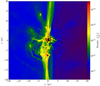 |
Fig. 1 Snapshot of an infant Pop III star cluster obtained with ENZO. We utilized these data to construct models of the assembly and further evolution of embedded Pop III star clusters. |
2.2 Models for the evolution of a Pop III star cluster
We took the positions, velocities, masses, and accretion rates of Pop III stars, along with the mass of the parent gas cloud and the gas inflow rate into the cluster, from the ENZO simulation. These were then used to perform N-body simulations within the AMUSE framework. We modeled six different Pop III star clusters based on the ENZO simulation output, which are listed in Table 1. To account for the effect of gas, we modeled it as a background analytic potential and increase its strength in proportion to the gas inflow rate. For unresolved SF, we assumed three different SF efficiencies - 10%, 20%, and 30% - to decide the total stellar mass. We also included gas accretion onto the stars, using mass-radius relations appropriate for Pop III stars (see Sect. 2.3), and considered stellar collisions and the associated mass loss (see Sect. 2.8). In total, we performed 18 simulations and evolved them for 2 Myr, which corresponds to the lifetime of the most massive Pop III star. The simulations were carried out using the AMUSE2 framework (see Portegies Zwart et al. 2009, 2013; Pelupessy et al. 2013; Portegies Zwart & McMillan 2018), by coupling the pure N-body code PH4 (McMillan & Hut 1996) with an analytic background potential using the BRIDGE method (Fujii et al. 2007). These processes are described in more detail below.
2.3 Mass-radius relation
To account for stellar growth, we used the mass-radius relation based on the work of Hosokawa & Omukai (2009) and Hosokawa et al. (2012, 2013). This relation is applicable to accreting protostars and main-sequence stars of primordial composition. For a detailed description, we refer the reader to Reinoso et al. (2023). In Fig. 2, we present the mass-radius relation for different mass accretion rates, along with the positions of the stars at the start of our simulations, which are taken from the ENZO run. We note that all stellar collisions in our simulations involve main-sequence stars only.
All the models with the corresponding parameters.
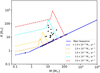 |
Fig. 2 Mass-radius relations for accreting Pop III stars. Dashed lines show the relations followed by protostars accreting at different rates, and the solid blue line is the relation followed by main sequence stars. The filled circles show the mass and radius for each particle at the beginning of our simulations. The stellar radii for the black circles were obtained with the accretion rates provided by ENZO, whereas the stellar radii for the red circles were obtained assuming ṁ = 0.0 M⊙/yr. |
2.4 The background potential
To model the gravitational effects of the gas on the cluster, we employed an analytic background potential of the form described in Binney & Tremaine (2008):
 (1)
(1)
and the enclosed mass given as
 (2)
(2)
We set  , r0 = 0.6 pc, and α = 1.1, to match the enclosed mass at 2 pc from the ENZO run, as shown in Fig. 3.
We further mimic gas accretion onto the cluster by modifying ρ0 as follows:
 (3)
(3)
and
 (4)
(4)
with r = 2 pc and Ṁgas = 2 M⊙ yr −1 taken from the ENZO run. This results in a value of  , which is used as the inflow rate for five models. We also explored a case with a higher inflow rate of Ṁgas = 0.9 M⊙ yr−1 at r = 1 pc, resulting in
  .
.
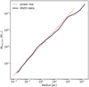 |
Fig. 3 Radial profile of the enclosed gas mass at the end of the ENZO run (solid black line), along with the enclosed mass for the power-law potential given by Eq. (1) (dotted red line), which is used as a background potential to mimic the gas in our models. |
2.5 The IMF
We constructed an IMF based on the output of the ENZO run and used it for all models. For this purpose, we employed a (four-part) power law of the form
 (5)
(5)
where

We present the comparison of constructed power law IMF with the ENZO output in Fig. 4.
To account for unresolved or subsequent SF, we assume a fixed SF efficiency (εSF) for 2 Myr. This determines the total stellar mass for our models as  . By varying εSF, we obtain three different values for MIMF. The adopted values of εSF and the resulting MIMF are listed in Table 1.
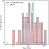 |
Fig. 4 Comparison of the IMF at the end of the ENZO run, with a sampling of the four-part power law IMF defined in Eq. (5). Both samples contain a total mass of 1497 M⊙ distributed among 68 particles. The four-part power law IMF is used to draw stars during SF episodes in our simulations. |
2.6 Star formation
For five of our models, we treated SF as a continuous process lasting for tSF = 2 Myr, which we refer to as continuous SF models. New stars were inserted into the simulation at time-intervals of
 (6)
(6)
with MSF = 200 M⊙ being the total mass in newly formed stars. The value of MSF was set to be higher than the maximum mass in the adopted IMF, ensuring that high-mass stars can also be created. For εSF = 0.1, dtSF = 1000 yr. We also included a model for which the SF process lasts for only tSF = 0.5 Myr, which we refer to as the rapid SF model. We achieved this by fixing dtSF = 1000 yr and allowing a maximum mass of MSF = 800 M⊙ per SF episode such that the same total number of stars are formed but in a shorter time span.
During the simulations we defined the star formation efficiency as
 (7)
(7)
where Mgas,2 is the gas mass enclosed within the central 2 pc, and Mstars is the current stellar mass. The amount of gas that is converted into new stars Mnew stars was defined as
 (8)
(8)
where εSF is the SF efficiency assumed for our model, as presented in Table 1. The use of εSF now allowed us to maintain a SF efficiency close to εSF during the entire simulation.
Once the total mass in new stars has been decided, we drew stars from the IMF until the required mass had been reached. A safety check was imposed such that if Mnew stars > Mgas,2, then star formation was postponed to the next timestep.
The newly formed stars were initialized with a Plummer density profile (Plummer 1911) with a Rv = 1.0 pc (scale length a = 0.589 pc) and in virial equilibrium, considering all the mass enclosed within 1 pc. We also imposed a cutoff radius of rcut = 3.5a = 2.06 pc to prevent new stars from forming too far from the cluster center. The mass transformed into stars was removed from the background potential by modifying ρ0 as follows:
 (9)
(9)
with r = 2 pc.
2.7 Gas accretion by individual stars
We modeled gas accretion onto the individual stars by assuming the Bondi-Hoyle-Lyttleton accretion rate. For this, we first calculated the Bondi radius as follows:
 (10)
(10)
where m is the mass of the accreting star, v is the velocity of the star, and cs is the sound speed. For the sound speed, we assumed constant values of γ = 5/3, T = 200 K, and μ = 1.43. The Bondi radius was used to calculate the accretion rate as
 (11)
(11)
where r is the radial position of the accreting star. The use of the Bondi radius prevents a singularity at r = 0. The accretion rate was recalculated at each timestep and an upper limit of  was imposed for main sequence stars. We also considered one model in which we set
  . The accreted mass was removed from the background potential by modifying ρ0.
To prevent dramatic changes in individual stellar masses, we used an adaptive timestep approach that imposes a maximum mass increase of 10 M⊙ per timestep. At the end of each timestep, the required timestep was computed as follows:
 (12)
(12)
where max(ṁi) is the maximum accretion rate among all the stars. If dtreq ≤ dt, the current timestep is modified as
 (13)
(13)
where j is the minimum integer for which the condition dtnew < dtreq is fulfilled. On the other hand, if dtreq ≥ 2dt, then dtnew = 2dt. We note that this timestep reduction is rarely triggered in our simulations and is only relevant for high-mass stars.
2.8 Stellar collisions and the associated mass loss
Stellar collisions are detected during the integration with the N-body code PH4. A stellar collision occurs if
 (14)
(14)
where d is the separation between two stars, and R1 and R2 are the stellar radii. Once a stellar collision was detected, we replaced the colliding particles with a new particle placed at the center of mass, with a velocity calculated assuming linear momentum conservation. We included a mass loss recipe based on the work of Glebbeek et al. (2013). The mass loss depends on the mass ratio q = m1/m2 (with m2 ≥ m1) and on the stellar structure through the parameters R0.86 and R0.5, which represent the radii containing 86% and 50% of the stellar mass, respectively. We assumed that all merging stars are on the main sequence and model them as n = 3 polytropes to obtain the required parameters. Using this approach, the fraction of mass lost during a collision can be calculated as follows:
 (15)
(15)
The mass of the collision product is estimated as
 (16)
(16)
The mass lost during the collision is also assumed to be lost from the system. The stellar radius of newly formed star is calculated using the mass radius relation in Sect. 2.3, with the accretion rate taken as the maximum of accretion rate among the colliding stars.
3 Results
We present here the main findings of our models, beginning with a description of the evolution of the star clusters and the formation of the most massive objects (MMOs). We then discuss the processes that lead to variations in the final masses of the MMOs.
3.1 Cluster and core contraction
Our simulations show a continuous contraction of the cluster core in all models. However, we note that the contraction rate depends on the εSF and the timescale over which SF occurs. In Fig. 5, we present the Lagrangian radii of our simulated clusters as a function of time for different models. Each line represents the average of three simulations, with the shaded region indicating one-sigma errors. A clear difference is immediately apparent in model E6 with rapid SF, where the clusters undergo core collapse, as traced by the 10% Lagrangian radius. For the remaining models, the clusters contract globally and continuously without reaching core collapse.
We also compared the contraction rates of the clusters by fitting an exponential function of the form
 (17)
(17)
to the 10% Lagrangian radii, for all the clusters. Here a and b are constants to be determined by the fit. The fit is performed between 0.25 and 1.25 Myr for all clusters, except for the models with rapid SF, where we selected the interval 0.25-0.6 Myr to avoid the core collapse phase, as illustrated in Fig. 5. The parameter a indicates the contraction rate of the cluster. We find that the contraction rate is anticorrelated with εSF, i.e., meaning faster contraction occurs for lower εSF. This result can be understood in terms of the relaxation timescale of a star cluster, which is given by (Spitzer 1987)
 (18)
(18)
with N being the number of stars and tcross the crossing time. We therefore expect trh to be longer in a cluster with more stars (provided tcross remains unchanged). Thus, when εSF is higher, N is larger and trh is longer. We also find that the contraction rate between 0.25 and 0.6 Myr is slower in clusters with rapid SF. The same argument applies here; the number of stars during the time span considered for this analysis is higher, which increases the relaxation time. As a result, the cluster contracts more slowly.
For the case of a higher gas inflow rate into the cluster, i.e., model E5 ( ), we also see a lower contraction rate for the cluster core. Two factors contribute to this effect. On one hand, the gas reservoir grows more rapidly, leading to more frequent episodes of SF, as implied by Eq. (6). This results in a larger N at any given time, thus increasing the relaxation timescale and slowing the core contraction. On the other hand, a higher gas inflow rate leads to more massive clusters, where stellar velocities are higher compared to those in clusters with lower inflow rates (Kroupa et al. 2020). Higher stellar velocities delay the relaxation processes (Reinoso et al. 2020), further slowing the core contraction rate.
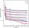 |
Fig. 5 Lagrangian radius evolution of some star cluster models. Solid lines represent the average of three simulations, and the shaded area represents one sigma errors. A fit to the core radius of the form Rc = beat is shown with a dashed brown line. We find that the core contraction rate depends on the SF efficiency. Additionally, we see the signature of a core collapse for models in which all stars form in a shorter time span (E6). |
3.2 Core collapse of clusters with rapid star formation
From Fig. 5 it is clear that for clusters with rapid SF, a core collapse occurs at around 1.75 Myr. This effect is also evident in the average mass of the MMO in Table 1. The only difference between models E1 and E6 is the timescale over which SF occurs, yet there is a factor of ~10 difference in the mass of the MMO. This difference arises from core collapse, which increases stellar density and, consequently, the number of collisions, as shown in Fig. 6. We note that the cores of clusters with rapid SF tend to be more compact even before the onset of core collapse, which increases the collision probability, as reflected in Fig. 6. Additionally, the first collisions tend to occur between 0.25 and 0.75 Myr for clusters with rapid SF, while they tend to occur later, between 1.25 and 1.5 Myr, for clusters with continuous SF. The high collision rate seen at ~1.75 Myr in Fig. 6 is also a distinctive feature of the core collapse in star clusters that triggers a runaway collision process (see, e.g., Portegies Zwart et al. 2004; Sakurai et al. 2017; Reinoso et al. 2020; Vergara et al. 2023).
Now, we explain why a core collapse occurs when SF is rapid. It is important to recall that in our model, stars are initialized with a Plummer density profile with Rv =1 pc, and in virial equilibrium, accounting for all the mass enclosed within the central parsec. From the virial theorem σν ∝ M, meaning that the larger the mass enclosed, the higher the velocity dispersion of the newly formed stars. This implies that for higher εSF, σν increases more rapidly, as shown in Fig. 7. For clusters with rapid SF, the vrms of stars in the core no longer increases as quickly once SF ceases. We interpret this result as follows: the continuous injection of stars in virial equilibrium effectively provides a source of kinetic energy into the cluster. Once this source is removed, the velocity changes of the stars are driven solely by the growing background potential and two-body relaxation effects with existing stars. Without this continuous kinetic energy injection, the clusters are able to undergo relaxation, which can lead to core collapse in a shorter timescale.
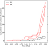 |
Fig. 6 Cumulative number of collisions as a function of time for two models that differ only in the timescale over which SF occurs. We see the signature of runaway stellar collisions in clusters for which SF occurs in a shorter time span. |
3.3 Emergence of the most massive object
In all our simulations, we find that the object that becomes the MMO forms early, within the first 50 kyr of evolution, and is formed outside the cluster core but within the half-mass radius. This object initially has a mass ranging from 80-150 M⊙, i.e., in the high-mass end of the IMF, and gradually sinks to the cluster core. An example of this process for different simulations is presented in Fig. 8. For  , the MMO consistently gains a total of 100-200 M⊙ through gas accretion, while the remainder of its mass growth comes from collisions with other stars as shown in Fig. 9. The relative contribution from accretion (collisions) is lower (higher) for more massive objects. Collisions with the MMO tend to occur rather late in the simulation at te > 1.25 Myr.
Our simulations show that most of the stars in the high-mass end of the IMF, i.e., with an initial mass M > 100 M⊙, typically form outside the core and therefore never experience a collision. In fact, the fraction of these stars that survive until the end of the simulation is typically >98%. Moreover, stars that experience a collision are typically the ones that are formed in between the cluster core and the half-mass radius, whereas the majority of the stars formed in the core (≳90%) survive until the end of the simulation. This means that even though the collisions occur in the cluster core, the colliding stars are typically formed outside. This is somewhat different in model E6, in which the clusters experience core collapse. In this case, the survival rate of M > 100 M⊙ stars is ~95%, and the majority of the high mass stars in the core (>60%) experience a collision.
The stochastic nature of stellar collisions makes it difficult to identify a single factor that can predict which object will become the MMO. Moreover, it is always a collision with a star of similar mass that marks the emergence of the MMO in the core. As shown in Fig. 10, we find that our star cluster models produce stars with masses greater than 103 M⊙ when εSF ≥ 0.3, or when a burst of SF assembles the cluster in ≤0.5 Myr. If high accretion rates onto individual stars are sustained (i.e., E4 model), the MMO can reach masses ≥104 M⊙.
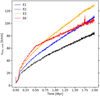 |
Fig. 7 Root-mean-square velocity of stars in the cluster core as a function of time for all the models with |

3.4 Higher accretion rate onto stars
Here, we present the case of a higher accretion rate onto the stars. Model E4 is identical to E1 except that its maximum accretion rate is ṁmax = 10−3 M⊙ yr−1. We note that the final mass of the MMO is approximately 30-40 times larger in E4. This is due to both a higher mass gained through accretion (by a factor of ~5) and a greater number of collisions (by a factor of ~8). Additionally, the typical mass of stars colliding with the MMO is around 1000 M⊙ due to the higher accretion rate.
The emergence of the MMO is similar to other models. A star with an initial mass of 70-120 M⊙ forms between the cluster core and the half-mass radius, and then sinks to the center as it gains mass through accretion. The key difference in this case is that the mass growth occurs much more rapidly, with the star typically gaining ~ 1400 M⊙ by accretion. Stellar collisions begin at earlier times, typically around 0.5-0.7 Myr, similar to the model with rapid SF. Notably, our results suggest that the onset of stellar collisions occurs once the number density of stars reaches 105 pc−3, with this quantity being a more reliable predictor than the stellar-mass density.
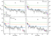 |
Fig. 8 Lagrangian radius evolution (10%, 50%, and 90%), radial position of the MMO (gray line), radial position at formation for stars that collide with the MMO (star symbols), and radial position of the same stars at the moment of the collision (filled circles) for simulations with different εSF and for a simulation with rapid SF (E6). In general, we see that the object that becomes the MMO is formed early on in the cluster evolution and rapidly sinks to the cluster core, where it eventually experiences the collisions that turn it into the MMO. The formation of the MMO is marked with a black star symbol. The moment at which SF ends is indicated by a vertical dashed black line. |
 |
Fig. 9 Fraction of the final mass gained through collisions (fcol), accretion (facc), and the initial mass (fini) for the MMO and second MMO, for models with different εSF. We present one simulation in each panel. In general, the initial mass is always in the range 80-150 M⊙, and the mass gained by accretion is always in the range 100-200 M⊙; the difference comes from the total mass gained through collisions. |
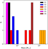 |
Fig. 10 Mass distribution of the MMOs formed in each of our models, including all three simulations per model. In general, the mass of the MMO increases with the SF efficiency, as well as with higher accretion rates onto stars (E4), or when all the stars are formed in a shorter time span (E6). |
3.5 MMOs in binary systems
We investigated whether the MMOs are part of a binary system at the end of the simulations. To do this, we first identified all the stars that are gravitationally bound to the MMO in the final snapshot. A pair of stars was considered gravitationally bound if their specific orbital energy (∊) is negative, as given by
 (19)
(19)
where v is the relative velocity, r is the distance between the pair, and μ = G(m1 + m2). We find that in most of our models, multiple stars are bound to the MMO. However, we are primarily interested in long-lived binary systems, not just gravitationally bound pairs. Therefore, we also considered the perturbations induced by the other stars as they can disrupt the binary system. To this end, we calculated a perturbation parameter, which we defined as
 (20)
(20)
where Fp,max is the maximum force acting on the primary star (i.e., the most massive one) due to the rest of the stars (excluding the secondary). Fs,max is analogous to Fp,max but for the secondary star. Fp,s is the gravitational force between the primary and secondary star.
To classify a bound pair as an unperturbed binary, we imposed the condition γ < 0.1, which ensures that we were considering pairs of particles that are dynamically separated from the rest of the system. We note that this perturbation parameter has been previously used to determine when to apply regularization in the NBODY code series (Aarseth 1999; Spurzem 1999; Wang et al. 2015; Nitadori & Aarseth 2012; Kamlah et al. 2022). Another criterion for selecting potentially long-lived binaries is to compare the binary’s semimajor axis to the hard-soft boundary aHS, which we computed as
 (21)
(21)
with M being the mass of the MMO, and vvrms,01 the root-meansquare velocity of all the stars in a sphere of r = 0.1 pc centered on the MMO. In general, hard binaries (a < aHS) tend to harden, while soft binaries (a > aHS) tend to soften (Heggie 1975; Hills 1975). We therefore also imposed the condition a/aHS < 1 in order to classify the pair as a potentially long-lived binary.
In Table 2, we list the number of stars bound to the MMO, the minimum value of γ among the bound stars (γmin), the mass of the star for which γ = γmin, and the ratio a/aHS. Based on the adopted criteria, we identify only three potentially long-lived binaries in our simulations.
4 Conclusion and discussion
Our models of Pop III star clusters are based on realistic initial conditions taken directly from a cosmological simulation. We have developed a model for their subsequent assembly and evolution. We find that BHs of up to a few thousand solar masses are formed through this scenario. These BH seeds are heavier compared to the single Pop III remnant scenario. Additionally, the fact that the BH is embedded in a massive star cluster will further aid its sinking into the deep potential well of the galaxy (Mukherjee et al. 2025). In particular, we might expect the system of stars and BH to experience subsequent episodes of gas accretion. BHs in such environments have been shown to grow at rates that can exceed the Eddington limit, with e-folding times of 200-300 Myr (Partmann et al. 2025). This pathway therefore offers a promising alternative to the DCBH scenario. The higher abundance of BH seeds forming through this channel can explain the recently observed abundance of AGNs at high z as found in high-resolution cosmological simulations (Mayer et al. 2025), along with the potential for further efficient growth. However, certain effects are still not included in our models, and we discuss some of these caveats below.
We have neglected mass loss due to stellar winds, given the zero metallicity of the stars considered in our models (Krtićka & Kubát 2006). It is worth noting that although rotating Pop III star models experience mass loss through winds, this only occurs once the stars become red giants (Meynet et al. 2006). Therefore, our results are robust against this effect, particularly with respect to the final masses of BHs, which would form via direct collapse (Heger et al. 2003). We did not include the effect of dynamical friction in our models either. Doing so would lead to a faster sinking of massive stars into the cluster core and subsequently may increase the total number of collisions. This may ultimately increase the mass of the MMO.
We have also neglected the stellar feedback during AMUSE simulations, which could increase the gas temperature and prevent further SF. However, previous studies show that the SN feedback is unable to expel the gas from massive embedded star clusters (Krause et al. 2016; Grudić et al. 2018; Lahén et al. 2025). Moreover, SF can still continue in such a system despite pre-SN feedback since the gas forms a disk in the cluster core (Lahén et al. 2025). Therefore, we expect that our results would not be changed significantly by such effects.
Perhaps one of the most surprising results of this study is that the continuous insertion of stars during the simulation (to mimic SF) delays the core-collapse of the star clusters. This effect is related to the numerical modeling as we assumed all newborn stars to be in virial equilibrium. This must be considered in future models. One potential way to mitigate this is to relax the assumption of virial equilibrium when inserting new stars and instead assume some degree of sub-viriality. For our models, this would likely result in clusters that can reach core-collapse within 2 Myr, triggering a runaway collision growth of the MMO and increasing the final masses of the BHs. In this regard, our results likely represent a lower limit on the mass of the BHs.
We evolved our simulations only up to 2 Myrs, as stellar evolution was not included, and thus we are unable to reliably track the fate of the remnants that form at this stage. However, we can assume that each MMO evolves into a BH of the same mass, with further growth possible through tidal disruption events (TDEs). Sakurai et al. (2019) explored the role of TDEs during BH growth in dense star clusters and found that the TDE rate is
 (22)
(22)
In our model with less favorable conditions, we have MBH ~ 400 M⊙, implying ~2 TDEs per megayear. For our model with MBH ~ 5000 M⊙, we get ~7 TDEs per megayear. In the most optimistic scenario, where 100 M⊙ stars are completely accreted, we might expect an increase of 200 to 700 M⊙ in the mass of these BHs. Thus, our results likely represent a lower limit for the final BH masses.
An important aspect to consider is the retention of BHs in the star clusters, as subsequent BH mergers can result in high-velocity recoil kicks. We estimated the recoil velocities by assuming that the two MMOs in each cluster will merge. These objects tend to form binary systems, and their typical masses are presented in Table 2. Our estimates are based on the fitting formulae provided by Merritt et al. (2004).
We began by considering our less massive clusters, which contain a total mass of 4 × 10⁵ M⊙ and a corresponding escape velocity of ~76 km s−1. In these clusters, the second MMO lies in the pair-instability supernova (PISN) mass range, so we considered a merger between BHs with masses of 420 and 140 M⊙. The recoil velocity ranges from 29 to 429 km s−1, indicating that BH ejection is possible in this case. For our clusters with a total mass of 6× 10⁵ M⊙, the escape velocity is 108 km s−1. The recoil velocities range from 10 to 235 km s−1 for the pair with 1000 and 754 M⊙, 24 to 352 km s−1 for the pair with 591 and 329 M⊙, and 3 to 68 km s−1 for the pair with 140 and 2317 M⊙. In this case, BH retention is almost certain for one pair but remains uncertain for the other two. For our clusters with a total mass of 1 × 10⁶ M⊙, the escape velocity is 132 km s−1. The recoil velocities range from 2 to 27 km s−1 for the pair with 3950 and 140 M⊙, 26 to 398 km s−1 for the pair with 532, and 140 M⊙, and 4 to 69 km s−1 for the pair with 2317 and 140 M⊙. In this case, it is highly likely that these clusters will retain their massive BHs. Next, we considered the clusters with rapid SF, which have a stellar mass of 4 × 10⁵ M⊙ and an escape velocity of 76 km s−1. The recoil velocities range from 5 to 88 km s−1 for the pair with 4227 and 335 M⊙, 1 to 20 km s−1 for the pair with 4699, and 140 M⊙, and 1 to 20 km s−1 for the pair with 4685 and 140M⊙. Again, it is very likely that these clusters will retain their massive BHs.
Ideally, one would need to follow the dynamical evolution of these BHs and their spins over longer timescales, as in Rantala et al. (2024). All of these BHs could grow further through TDEs and if the new stars are initialized in a sub-virial state; as discussed above, the final BH masses could be a factor of ~10 higher. This increase in mass would drastically reduce the recoil kick velocity, meaning that all of these BHs would most likely be retained in their clusters. In general, our simple estimates suggest that the most massive clusters are highly likely to retain their BHs as they merge with other significantly less massive BHs.
Parameters related to the identification of binary systems that involve the MMO in each simulation.
Acknowledgements
We gratefully acknowledge the Federal Ministry of Education and Research and the state governments of Chile for supporting this project as part of the funding of the Kultrun cluster hosted at the Departamento de Astronomía, Universidad de Concepción. BR acknowledges funding through ANID (CONICYT-PFCHA/Doctorado acuerdo bilateral DAAD/62180013), DAAD (funding program number 57451854), the International Max Planck Research School for Astronomy and Cosmic Physics at the University of Heidelberg (IMPRS-HD), and the support by the European Research Council via ERC Consolidator grant KETJU (no. 818930). DRGS thanks for funding via the Alexander von Humboldt - Foundation, Bonn, Germany and the ANID BASAL project FB210003.
Appendix A Orbital parameters that led to stellar collisions
In this section we present a compilation of orbital parameters for several pairs of stars that collide in our simulations. For each of the collisions in our simulations we searched for the colliding stars in the snapshot just prior to the event. We then calculated the specific orbital energy of the pair and computed the orbital parameters. Finally, we calculated the pericenter distance rp of the orbit. For all the systems in which rp ≤ R1 + R2, we presumed that the orbit derived from this analysis is the orbit that finally led to the stellar collision. We present in Table A.1 the orbital parameters for all these systems, as they serve for producing realistic initial conditions for the study of stellar collisions between massive stars in dense star clusters.
Subset of collisions from our simulations.
Appendix B Gas inflow and halo growth
The gaseous collapse in the mini-halo was prevented in a similar fashion as in Latif et al. (2022b), and cold dense gas inflows resulted in rapid gas accretion, as shown in Fig. B.1. Turbulent motions prevented gas infall until the halo grew to a few times 107 M⊙ and large inflow velocities overcame the turbulent motions leading to catastrophic collapse (see Fig. B.2). We also present a snapshot of the halo on a scale of the virial radius in Fig. B.3.
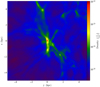 |
Fig. B.1 Large-scale view of the halo showing its environment and cold dense streams of gas that drive turbulent motions at the center. |
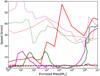 |
Fig. B.2 Gas velocity profiles versus the enclosed mass. Dotted lines show the turbulent velocities, solid lines the infall velocities, and dashed lines thermal sound speeds. Magenta, green, and red colors show time evolution, from earlier to later times. |
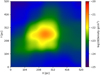 |
Fig. B.3 View of the halo on a scale corresponding to the virial radius, which is equal to 260 pc. |
References
- Aarseth, S. J. 1999, PASP, 111, 1333 [NASA ADS] [CrossRef] [Google Scholar]
- Abel, T., Anninos, P., Zhang, Y., & Norman, M. L. 1997, New Astron., 2, 181 [NASA ADS] [CrossRef] [Google Scholar]
- Adamo, A., Bradley, L. D., Vanzella, E., et al. 2024, Nature, 632, 513 [NASA ADS] [CrossRef] [Google Scholar]
- Alvarez, M. A., Wise, J. H., & Abel, T. 2009, ApJ, 701, L133 [NASA ADS] [CrossRef] [Google Scholar]
- Arca Sedda, M., Kamlah, A. W. H., Spurzem, R., et al. 2023, MNRAS, 526, 429 [NASA ADS] [CrossRef] [Google Scholar]
- Arca Sedda, M., Kamlah, A. W. H., Spurzem, R., et al. 2024, MNRAS, 528, 5119 [NASA ADS] [CrossRef] [Google Scholar]
- Banados, E., Venemans, B. P., Mazzucchelli, C., et al. 2018, Nature, 553, 473 [NASA ADS] [CrossRef] [Google Scholar]
- Bañados, E., Mazzucchelli, C., Momjian, E., et al. 2021, ApJ, 909, 80 [CrossRef] [Google Scholar]
- Behroozi, P. S., Wechsler, R. H., & Wu, H.-Y. 2013, ApJ, 762, 109 [NASA ADS] [CrossRef] [Google Scholar]
- Binney, J., & Tremaine, S. 2008, Galactic Dynamics, 2nd edn. [Google Scholar]
- Boekholt, T. C. N., Schleicher, D. R. G., Fellhauer, M., et al. 2018, MNRAS, 476, 366 [Google Scholar]
- Bogdán, A., Goulding, A. D., Natarajan, P., et al. 2024, Nat. Astron., 8, 126 [Google Scholar]
- Bovino, S., Latif, M. A., Grassi, T., & Schleicher, D. R. G. 2014, MNRAS, 441, 2181 [Google Scholar]
- Bryan, G. L., Norman, M. L., O’Shea, B. W., et al. 2014, ApJS, 211, 19 [Google Scholar]
- Chon, S., & Omukai, K. 2020, MNRAS, 494, 2851 [Google Scholar]
- Chon, S., & Omukai, K. 2025, MNRAS, 539, 2561 [Google Scholar]
- Chon, S., Hosokawa, T., & Yoshida, N. 2018, MNRAS, 475, 4104 [CrossRef] [Google Scholar]
- Davies, M. B., Miller, M. C., & Bellovary, J. M. 2011, ApJ, 740, L42 [NASA ADS] [CrossRef] [Google Scholar]
- Escala, A. 2021, ApJ, 908, 57 [NASA ADS] [CrossRef] [Google Scholar]
- Fan, X., Strauss, M. A., Richards, G. T., et al. 2006, AJ, 131, 1203 [NASA ADS] [CrossRef] [Google Scholar]
- Federrath, C., Sur, S., Schleicher, D. R. G., Banerjee, R., & Klessen, R. S. 2011, ApJ, 731, 62 [NASA ADS] [CrossRef] [Google Scholar]
- Fujii, M., Iwasawa, M., Funato, Y., & Makino, J. 2007, PASJ, 59, 1095 [NASA ADS] [Google Scholar]
- Furtak, L. J., Labbé, I., Zitrin, A., et al. 2024, Nature, 628, 57 [NASA ADS] [CrossRef] [Google Scholar]
- Gaete, B., Schleicher, D. R. G., Lupi, A., et al. 2024, A&A, 690, A378 [NASA ADS] [CrossRef] [EDP Sciences] [Google Scholar]
- Giersz, M., Askar, A., Hypki, A., et al. 2025, A&A, 699, A76 [NASA ADS] [CrossRef] [EDP Sciences] [Google Scholar]
- Glebbeek, E., Gaburov, E., Portegies Zwart, S., & Pols, O. R. 2013, MNRAS, 434, 3497 [NASA ADS] [CrossRef] [Google Scholar]
- Goulding, A. D., Greene, J. E., Setton, D. J., et al. 2023, ApJ, 955, L24 [NASA ADS] [CrossRef] [Google Scholar]
- Greene, J. E., Labbe, I., Goulding, A. D., et al. 2024, ApJ, 964, 39 [CrossRef] [Google Scholar]
- Greif, T. H., Johnson, J. L., Klessen, R. S., & Bromm, V. 2008, MNRAS, 387, 1021 [NASA ADS] [CrossRef] [Google Scholar]
- Grudic, M. Y., Hopkins, P. F., Quataert, E., & Murray, N. 2018, MNRAS, 483, 5548 [Google Scholar]
- Habouzit, M., Volonteri, M., Latif, M., Dubois, Y., & Peirani, S. 2016, MNRAS, 463, 529 [NASA ADS] [CrossRef] [Google Scholar]
- Hahn, O., & Abel, T. 2011, MNRAS, 415, 2101 [Google Scholar]
- Heger, A., Fryer, C. L., Woosley, S. E., Langer, N., & Hartmann, D. H. 2003, ApJ, 591, 288 [CrossRef] [Google Scholar]
- Heggie, D. C. 1975, MNRAS, 173, 729 [NASA ADS] [CrossRef] [Google Scholar]
- Hills, J. G. 1975, AJ, 80, 809 [NASA ADS] [CrossRef] [Google Scholar]
- Hirano, S., Hosokawa, T., Yoshida, N., & Kuiper, R. 2017, Science, 357, 1375 [CrossRef] [Google Scholar]
- Hosokawa, T., & Omukai, K. 2009, ApJ, 703, 1810 [NASA ADS] [CrossRef] [Google Scholar]
- Hosokawa, T., Omukai, K., & Yorke, H. W. 2012, ApJ, 756, 93 [Google Scholar]
- Hosokawa, T., Yorke, H. W., Inayoshi, K., Omukai, K., & Yoshida, N. 2013, ApJ, 778, 178 [Google Scholar]
- Johnson, J. L., & Bromm, V. 2007, MNRAS, 374, 1557 [NASA ADS] [CrossRef] [Google Scholar]
- Kamlah, A. W. H., Leveque, A., Spurzem, R., et al. 2022, MNRAS, 511, 4060 [NASA ADS] [CrossRef] [Google Scholar]
- Katz, H., Sijacki, D., & Haehnelt, M. G. 2015, MNRAS, 451, 2352 [Google Scholar]
- King, A. 2024, MNRAS, 531, 550 [NASA ADS] [CrossRef] [Google Scholar]
- Kocevski, D. D., Finkelstein, S. L., Barro, G., et al. 2025, ApJ, 986, 126 [Google Scholar]
- Kokorev, V., Fujimoto, S., Labbe, I., et al. 2023, ApJ, 957, L7 [NASA ADS] [CrossRef] [Google Scholar]
- Kokorev, V., Caputi, K. I., Greene, J. E., et al. 2024, ApJ, 968, 38 [NASA ADS] [CrossRef] [Google Scholar]
- Kovács, O. E., Bogdán, A., Natarajan, P., et al. 2024, ApJ, 965, L21 [CrossRef] [Google Scholar]
- Krause, M. G. H., Charbonnel, C., Bastian, N., & Diehl, R. 2016, A&A, 587, A53 [NASA ADS] [CrossRef] [EDP Sciences] [Google Scholar]
- Kroupa, P., Subr, L., Jerabkova, T., & Wang, L. 2020, MNRAS, 498, 5652 [Google Scholar]
- Krtićka, J., & Kubát, J. 2006, A&A, 446, 1039 [NASA ADS] [CrossRef] [EDP Sciences] [Google Scholar]
- Lahén, N., Naab, T., Rantala, A., & Partmann, C. 2025, MNRAS, submitted, [arXiv:2504.18620] [Google Scholar]
- Lambrides, E., Chiaberge, M., Long, A. S., et al. 2024a, ApJ, 961, L25 [NASA ADS] [CrossRef] [Google Scholar]
- Lambrides, E., Garofali, K., Larson, R., et al. 2024b, arXiv e-prints, [arXiv:2409.13047] [Google Scholar]
- Larson, R. L., Finkelstein, S. L., Kocevski, D. D., et al. 2023, ApJ, 953, L29 [NASA ADS] [CrossRef] [Google Scholar]
- Latif, M. A., & Khochfar, S. 2020, MNRAS, 497, 3761 [Google Scholar]
- Latif, M. A., & Volonteri, M. 2015, MNRAS, 452, 1026 [CrossRef] [Google Scholar]
- Latif, M. A., Schleicher, D. R. G., Schmidt, W., & Niemeyer, J. 2013, MNRAS, 433, 1607 [NASA ADS] [CrossRef] [Google Scholar]
- Latif, M. A., Schleicher, D. R. G., Bovino, S., Grassi, T., & Spaans, M. 2014, ApJ, 792, 78 [NASA ADS] [CrossRef] [Google Scholar]
- Latif, M. A., Schleicher, D. R. G., & Hartwig, T. 2016, MNRAS, 458, 233 [NASA ADS] [CrossRef] [Google Scholar]
- Latif, M. A., Khochfar, S., Schleicher, D., & Whalen, D. J. 2021, MNRAS, 508, 1756 [NASA ADS] [CrossRef] [Google Scholar]
- Latif, M. A., Whalen, D., & Khochfar, S. 2022a, ApJ, 925, 28 [NASA ADS] [CrossRef] [Google Scholar]
- Latif, M. A., Whalen, D. J., Khochfar, S., Herrington, N. P., & Woods, T. E. 2022b, Nature, 607, 48 [CrossRef] [Google Scholar]
- Liempi, M., Schleicher, D. R. G., Benson, A., Escala, A., & Vergara, M. C. 2025, A&A, 694, A42 [NASA ADS] [CrossRef] [EDP Sciences] [Google Scholar]
- Lupi, A., Colpi, M., Devecchi, B., Galanti, G., & Volonteri, M. 2014, MNRAS, 442, 3616 [NASA ADS] [CrossRef] [Google Scholar]
- Lupi, A., Trinca, A., Volonteri, M., Dotti, M., & Mazzucchelli, C. 2024, A&A, 689, A128 [NASA ADS] [CrossRef] [EDP Sciences] [Google Scholar]
- Maio, U., Dolag, K., Ciardi, B., & Tornatore, L. 2007, MNRAS, 379, 963 [NASA ADS] [CrossRef] [Google Scholar]
- Maiolino, R., Scholtz, J., Witstok, J., et al. 2024, Nature, 627, 59 [NASA ADS] [CrossRef] [Google Scholar]
- Maiolino, R., Risaliti, G., Signorini, M., et al. 2025, MNRAS, 538, 1921 [Google Scholar]
- Matthee, J., Naidu, R. P., Brammer, G., et al. 2024, ApJ, 963, 129 [NASA ADS] [CrossRef] [Google Scholar]
- Mayer, L., van Donkelaar, F., Messa, M., Capelo, P. R., & Adamo, A. 2025, ApJ, 981, L28 [Google Scholar]
- McGreer, I. D., & Bryan, G. L. 2008, ApJ, 685, 8 [CrossRef] [Google Scholar]
- McMillan, S. L. W., & Hut, P. 1996, ApJ, 467, 348 [CrossRef] [Google Scholar]
- Merritt, D., Milosavljevic, M., Favata, M., Hughes, S. A., & Holz, D. E. 2004, ApJ, 607, L9 [NASA ADS] [CrossRef] [Google Scholar]
- Meynet, G., Ekström, S., & Maeder, A. 2006, A&A, 447, 623 [NASA ADS] [CrossRef] [EDP Sciences] [Google Scholar]
- Mirocha, J., Skory, S., Burns, J. O., & Wise, J. H. 2012, ApJ, 756, 94 [Google Scholar]
- Mortlock, D. J., Warren, S. J., Venemans, B. P., et al. 2011, Nature, 474, 616 [Google Scholar]
- Mukherjee, D., Zhou, Y., Chen, N., Di Carlo, U. N., & Di Matteo, T. 2025, ApJ, 981, 203 [Google Scholar]
- Naidu, R. P., Matthee, J., Katz, H., et al. 2025, arXiv e-prints, [arXiv:2503.16596] [Google Scholar]
- Napolitano, L., Castellano, M., Pentericci, L., et al. 2024, ApJ, submitted, [arXiv:2410.18763] [Google Scholar]
- Nitadori, K., & Aarseth, S. J. 2012, MNRAS, 424, 545 [NASA ADS] [CrossRef] [Google Scholar]
- O’Brennan, H., Regan, J. A., Brennan, J., et al. 2025, Open J. Astrophys., 8, 88 [Google Scholar]
- Omukai, K., Schneider, R., & Haiman, Z. 2008, ApJ, 686, 801 [Google Scholar]
- Onoue, M., Kashikawa, N., Matsuoka, Y., et al. 2019, ApJ, 880, 77 [Google Scholar]
- Pacucci, F., Natarajan, P., Volonteri, M., Cappelluti, N., & Urry, C. M. 2017, ApJ, 850, L42 [NASA ADS] [CrossRef] [Google Scholar]
- Partmann, C., Naab, T., Lahén, N., et al. 2025, MNRAS, 537, 956 [Google Scholar]
- Patrick, S. J., Whalen, D. J., Latif, M. A., & Elford, J. S. 2023, MNRAS, 522, 3795 [NASA ADS] [CrossRef] [Google Scholar]
- Pelupessy, F. I., van Elteren, A., de Vries, N., et al. 2013, A&A, 557, A84 [NASA ADS] [CrossRef] [EDP Sciences] [Google Scholar]
- Planck Collaboration XIII. 2016, A&A, 594, A13 [NASA ADS] [CrossRef] [EDP Sciences] [Google Scholar]
- Plummer, H. C. 1911, MNRAS, 71, 460 [Google Scholar]
- Portegies Zwart, S., & McMillan, S. 2018, Astrophysical Recipes; The art of AMUSE [Google Scholar]
- Portegies Zwart, S. F., Baumgardt, H., Hut, P., Makino, J., & McMillan, S. L. W. 2004, Nature, 428, 724 [Google Scholar]
- Portegies Zwart, S., McMillan, S., Harfst, S., et al. 2009, New A, 14, 369 [NASA ADS] [CrossRef] [Google Scholar]
- Portegies Zwart, S., McMillan, S. L. W., van Elteren, E., Pelupessy, I., & de Vries, N. 2013, Comput. Phys. Commun., 184, 456 [Google Scholar]
- Rantala, A., Naab, T., & Lahén, N. 2024, MNRAS, 531, 3770 [NASA ADS] [CrossRef] [Google Scholar]
- Reed, S. L., Banerji, M., Becker, G. D., et al. 2019, MNRAS, 487, 1874 [Google Scholar]
- Regan, J. A., & Downes, T. P. 2018, MNRAS, 475, 4636 [NASA ADS] [CrossRef] [Google Scholar]
- Regan, J. A., & Haehnelt, M. G. 2009a, MNRAS, 396, 343 [CrossRef] [Google Scholar]
- Regan, J. A., & Haehnelt, M. G. 2009b, MNRAS, 393, 858 [NASA ADS] [CrossRef] [Google Scholar]
- Regan, J., & Volonteri, M. 2024, Open J. Astrophys., 7, 72 [NASA ADS] [CrossRef] [Google Scholar]
- Regan, J. A., Wise, J. H., Woods, T. E., et al. 2020, Open J. Astrophys., 3, 15 [NASA ADS] [Google Scholar]
- Reinoso, B., Schleicher, D. R. G., Fellhauer, M., Klessen, R. S., & Boekholt, T. C. N. 2018, A&A, 614, A14 [NASA ADS] [CrossRef] [EDP Sciences] [Google Scholar]
- Reinoso, B., Schleicher, D. R. G., Fellhauer, M., Leigh, N. W. C., & Klessen, R. S. 2020, A&A, 639, A92 [NASA ADS] [CrossRef] [EDP Sciences] [Google Scholar]
- Reinoso, B., Klessen, R. S., Schleicher, D., Glover, S. C. O., & Solar, P. 2023, MNRAS, 521, 3553 [CrossRef] [Google Scholar]
- Rusakov, V., Watson, D., Nikopoulos, G. P., et al. 2025, Nature, submitted [arXiv:2503.16595] [Google Scholar]
- Saavedra-Bastidas, J., Schleicher, D. R. G., Klessen, R. S., et al. 2024, A&A, 690, A186 [NASA ADS] [CrossRef] [EDP Sciences] [Google Scholar]
- Sakurai, Y., Yoshida, N., Fujii, M. S., & Hirano, S. 2017, MNRAS, 472, 1677 [NASA ADS] [CrossRef] [Google Scholar]
- Sakurai, Y., Yoshida, N., & Fujii, M. S. 2019, MNRAS, 484, 4665 [Google Scholar]
- Sassano, F., Schneider, R., Valiante, R., et al. 2021, MNRAS, 506, 613 [CrossRef] [Google Scholar]
- Schaerer, D. 2002, A&A, 382, 28 [NASA ADS] [CrossRef] [EDP Sciences] [Google Scholar]
- Schleicher, D. R. G., Reinoso, B., Latif, M., et al. 2022, MNRAS, 512, 6192 [NASA ADS] [CrossRef] [Google Scholar]
- Schleicher, D. R. G., Reinoso, B., & Klessen, R. S. 2023, MNRAS, 521, 3972 [NASA ADS] [CrossRef] [Google Scholar]
- Schneider, R., Valiante, R., Trinca, A., et al. 2023, MNRAS, 526, 3250 [NASA ADS] [CrossRef] [Google Scholar]
- Smith, B. D., Regan, J. A., Downes, T. P., et al. 2018, MNRAS, 480, 3762 [NASA ADS] [CrossRef] [Google Scholar]
- Spitzer, L. 1987, Dynamical evolution of globular clusters [Google Scholar]
- Spurzem, R. 1999, J. Computat. Appl. Math., 109, 407 [Google Scholar]
- Tagawa, H., Haiman, Z., & Kocsis, B. 2020, ApJ, 892, 36 [Google Scholar]
- Trinca, A., Valiante, R., Schneider, R., et al. 2024, A&A, submitted [arXiv:2412.14248] [Google Scholar]
- Vergara, M. Z. C., Schleicher, D. R. G., Boekholt, T. C. N., et al. 2021, A&A, 649, A160 [NASA ADS] [CrossRef] [EDP Sciences] [Google Scholar]
- Vergara, M. C., Escala, A., Schleicher, D. R. G., & Reinoso, B. 2023, MNRAS, 522, 4224 [NASA ADS] [CrossRef] [Google Scholar]
- Vergara, M. C., Schleicher, D. R. G., Escala, A., et al. 2024, A&A, 689, A34 [NASA ADS] [CrossRef] [EDP Sciences] [Google Scholar]
- Wang, L., Spurzem, R., Aarseth, S., et al. 2015, MNRAS, 450, 4070 [NASA ADS] [CrossRef] [Google Scholar]
- Wang, F., Yang, J., Fan, X., et al. 2021, ApJ, 907, L1 [Google Scholar]
- Wise, J. H., Regan, J. A., O’Shea, B. W., et al. 2019, Nature, 566, 85 [NASA ADS] [CrossRef] [Google Scholar]
- Woods, T. E., Heger, A., Whalen, D. J., Haemmerlé, L., & Klessen, R. S. 2017, ApJ, 842, L6 [Google Scholar]
- Wu, X.-B., Wang, F., Fan, X., et al. 2015, Nature, 518, 512 [Google Scholar]
- Yoshida, N., Omukai, K., & Hernquist, L. 2007, ApJ, 667, L117 [NASA ADS] [CrossRef] [Google Scholar]
See https://github.com/jwise77/enzo-mrp-music for details.
All Tables
Parameters related to the identification of binary systems that involve the MMO in each simulation.
All Figures
|
Fig. 1 Snapshot of an infant Pop III star cluster obtained with ENZO. We utilized these data to construct models of the assembly and further evolution of embedded Pop III star clusters. |
| In the text | |
|
Fig. 2 Mass-radius relations for accreting Pop III stars. Dashed lines show the relations followed by protostars accreting at different rates, and the solid blue line is the relation followed by main sequence stars. The filled circles show the mass and radius for each particle at the beginning of our simulations. The stellar radii for the black circles were obtained with the accretion rates provided by ENZO, whereas the stellar radii for the red circles were obtained assuming ṁ = 0.0 M⊙/yr. |
| In the text | |
|
Fig. 3 Radial profile of the enclosed gas mass at the end of the ENZO run (solid black line), along with the enclosed mass for the power-law potential given by Eq. (1) (dotted red line), which is used as a background potential to mimic the gas in our models. |
| In the text | |
|
Fig. 4 Comparison of the IMF at the end of the ENZO run, with a sampling of the four-part power law IMF defined in Eq. (5). Both samples contain a total mass of 1497 M⊙ distributed among 68 particles. The four-part power law IMF is used to draw stars during SF episodes in our simulations. |
| In the text | |
|
Fig. 5 Lagrangian radius evolution of some star cluster models. Solid lines represent the average of three simulations, and the shaded area represents one sigma errors. A fit to the core radius of the form Rc = beat is shown with a dashed brown line. We find that the core contraction rate depends on the SF efficiency. Additionally, we see the signature of a core collapse for models in which all stars form in a shorter time span (E6). |
| In the text | |
|
Fig. 6 Cumulative number of collisions as a function of time for two models that differ only in the timescale over which SF occurs. We see the signature of runaway stellar collisions in clusters for which SF occurs in a shorter time span. |
| In the text | |
|
Fig. 7 Root-mean-square velocity of stars in the cluster core as a function of time for all the models with |
| In the text | |
|
Fig. 8 Lagrangian radius evolution (10%, 50%, and 90%), radial position of the MMO (gray line), radial position at formation for stars that collide with the MMO (star symbols), and radial position of the same stars at the moment of the collision (filled circles) for simulations with different εSF and for a simulation with rapid SF (E6). In general, we see that the object that becomes the MMO is formed early on in the cluster evolution and rapidly sinks to the cluster core, where it eventually experiences the collisions that turn it into the MMO. The formation of the MMO is marked with a black star symbol. The moment at which SF ends is indicated by a vertical dashed black line. |
| In the text | |
|
Fig. 9 Fraction of the final mass gained through collisions (fcol), accretion (facc), and the initial mass (fini) for the MMO and second MMO, for models with different εSF. We present one simulation in each panel. In general, the initial mass is always in the range 80-150 M⊙, and the mass gained by accretion is always in the range 100-200 M⊙; the difference comes from the total mass gained through collisions. |
| In the text | |
|
Fig. 10 Mass distribution of the MMOs formed in each of our models, including all three simulations per model. In general, the mass of the MMO increases with the SF efficiency, as well as with higher accretion rates onto stars (E4), or when all the stars are formed in a shorter time span (E6). |
| In the text | |
|
Fig. B.1 Large-scale view of the halo showing its environment and cold dense streams of gas that drive turbulent motions at the center. |
| In the text | |
|
Fig. B.2 Gas velocity profiles versus the enclosed mass. Dotted lines show the turbulent velocities, solid lines the infall velocities, and dashed lines thermal sound speeds. Magenta, green, and red colors show time evolution, from earlier to later times. |
| In the text | |
|
Fig. B.3 View of the halo on a scale corresponding to the virial radius, which is equal to 260 pc. |
| In the text | |
Current usage metrics show cumulative count of Article Views (full-text article views including HTML views, PDF and ePub downloads, according to the available data) and Abstracts Views on Vision4Press platform.
Data correspond to usage on the plateform after 2015. The current usage metrics is available 48-96 hours after online publication and is updated daily on week days.
Initial download of the metrics may take a while.