| Issue |
A&A
Volume 700, August 2025
|
|
|---|---|---|
| Article Number | A221 | |
| Number of page(s) | 11 | |
| Section | Astronomical instrumentation | |
| DOI | https://doi.org/10.1051/0004-6361/202554903 | |
| Published online | 21 August 2025 | |
Faraday synthesis in direction-dependent imaging
1
Hamburger Sternwarte, Universität Hamburg,
Gojenbergsweg 112,
21029
Hamburg,
Germany
2
GEPI, Observatoire de Paris, Universié PSL, CNRS,
5 Place Jules Janssen,
92190
Meudon,
France
3
Department of Physics & Electronics, Rhodes University,
PO Box 94,
Grahamstown
6140,
South Africa
4
Max Planck Institute for Astrophysics,
Karl-Schwarzschild-Str. 1,
85748
Garching,
Germany
5
Deutsches Zentrum für Astrophysik,
Postplatz 1,
02826
Görlitz,
Germany
6
Ludwig-Maximilians-Universität München,
Geschwister-Scholl-Platz 1,
80539
Munich,
Germany
7
Excellence Cluster ORIGINS,
Boltzmannstr. 2,
85748
Garching,
Germany
8
Departamento de Física de la Tierra y Astrofísica & IPARCOS-UCM, Universidad Complutense de Madrid,
28040
Madrid,
Spain
9
INAF – Istituto di Radioastronomia,
via P. Gobetti 101,
40129
Bologna,
Italy
★ Corresponding author.
Received:
31
March
2025
Accepted:
25
June
2025
Abstract
Context. Modern radio interferometers enable high-resolution polarization imaging, providing insights into cosmic magnetism through rotation measure (RM) synthesis. Traditional 2+1D RM synthesis treats the 2D spatial transform and the 1D transform in frequency space separately. A fully three-dimensional approach transforms the data directly from two spatial frequencies and one wave frequency (u, υ, v) to sky-Faraday depth space, using a 3D Fourier transform. Faraday synthesis uses the entire dataset for improved reconstruction, but also requires a 3D deconvolution algorithm to subtract artifacts from the residual image. However, applying this method to modern interferometers requires corrections for direction-dependent effects (DDEs).
Aims. We extend Faraday synthesis by incorporating direction-dependent corrections, allowing for accurate polarized imaging in the presence of instrumental and ionospheric effects.
Methods. We implemented this method within DDFACET, introducing a direction-dependent deconvolution algorithm (DDFSCLEAN) that applies DDE corrections in a faceted framework. Additionally, we parametrized the CLEAN components and evaluated the model on a larger subset of frequency channels, naturally correcting for bandwidth depolarization. We tested our method on both synthetic and real interferometric data.
Results. Our results show that Faraday synthesis enables deeper deconvolution, reducing artifacts and increasing the dynamic range. The bandwidth depolarization correction improves the recovery of polarized flux, allowing coarser frequency resolution without losing sensitivity at high Faraday depths. From the 3D reconstruction, we also identified a polarized source in a LOFAR survey pointing that was not detected by previous RM surveys. Faraday synthesis is memory-intensive due to the large transforms between the visibility domain and the Faraday cube, and thus is only now becoming practical. Nevertheless, our implementation achieves comparable or faster runtimes than the 2+1D approach, making it a competitive alternative for polarization imaging.
Key words: magnetic fields / polarization / methods: data analysis / techniques: interferometric / techniques: polarimetric
© The Authors 2025
 Open Access article, published by EDP Sciences, under the terms of the Creative Commons Attribution License (https://creativecommons.org/licenses/by/4.0), which permits unrestricted use, distribution, and reproduction in any medium, provided the original work is properly cited.
This article is published in open access under the Subscribe to Open model. This email address is being protected from spambots. You need JavaScript enabled to view it. to support open access publication.
1 Introduction
Modern radio interferometers, such as MeerKAT (Jonas & MeerKAT Team 2016), the Australian Square Kilometre Array Pathfinder (ASKAP; Vanderwoude et al. 2024), the LOw Frequency ARray (LOFAR; van Haarlem et al. 2013), and the Expanded Very Large Array (EVLA; Perley et al. 2011), have enabled high-resolution, wide-field imaging across broad frequency ranges. Among their many applications, the study of linear polarization provides a unique window into the magnetic fields of astrophysical objects, as well as the intervening medium through which the radio waves they emit propagate (Anderson et al. 2024; Böckmann et al. 2023; O’Sullivan et al. 2023; De Rubeis et al. 2024, e.g.). Over the past two decades, Faraday rotation measure (RM) synthesis (Brentjens & de Bruyn 2005) has become an important technique to study magnetic fields in general, and cosmic magnetism in particular. This method decomposes the line-of-sight (LOS) Faraday rotating signal into its constituent components as a function of Faraday depth, defined as
 (1)
(1)
where ne is the net number density of thermal electrons and positrons, accounting for their opposite charges, and Bz is the LOS component of the magnetic field. Faraday depth quantifies the rate at which the polarization angle, χ, changes as the electric field vector of electromagnetic radiation rotates while propagating through a magnetized plasma. The amount of rotation at wavelength λ is given by
 (2)
(2)
where χ0 is the intrinsic polarization angle at the source of emission. In the simplest case, when there is a single Faraday rotating screen along the LOS and no internal Faraday rotation within the emitting source, the Faraday depth is equivalent to the rotation measure. In this scenario, as described by Burn (1966), the polarization angle varies linearly with the square of the wavelength, and the RM is defined as
 (3)
(3)
The RM synthesis algorithm is traditionally applied to each LOS independently of spatially deconvolved radio interferometric images, a technique we will refer to as 2+1D. Bell & Enßlin (2012) introduced a 3D framework called Faraday synthesis that unifies radio interferometric aperture synthesis with RM synthesis. This approach transforms data directly from baseline-frequency coordinates (u,υ,v) to sky-Faraday depth space (l, m, ϕ), using a 3D Fourier transform.
While a 2+1D Fourier transform is mathematically equivalent to a 3D Fourier transform, the image reconstructions from 2+1D RM synthesis and 3D Faraday synthesis are generally not equivalent. This is because both methods apply nonlinear operations to reconstruct unmeasured information-RM synthesis does so sequentially in 2D and 1D, while Faraday synthesis applies it in 3D – and these operations are not equivalent. Bell & Enßlin (2012) therefore introduced a novel deconvolution algorithm based on the CLEAN algorithm (Högbom 1974), called FSCLEAN, which uses full data-space sampling to construct a 3D point spread function (PSF) that is used to subtract artifacts from the residual image. Simultaneously, the model image is populated with point-source components in the sky-Faraday depth space, corresponding to the brightest point in the residual cube. Using a major-minor cycle scheme, as introduced by Clark (1980), the algorithm performs a series of minor iterations in the sky domain, followed by a transformation of the predicted sky model to data space, where the next set of residual visibilities are computed. This process is repeated multiple times, progressively refining the model until convergence is achieved and ensuring alignment between the sky model and the visibility-frequency data. Although this technique was able to achieve great improvements in dynamic range, spatial resolution, artifact reduction, and accurate reconstruction of low signal-to-noise sources, its adoption by the radio astronomy community has been limited. One challenge is adapting the method to modern interferometers, which require corrections for direction-dependent effects (DDEs), such as complex beam patterns and ionospheric Faraday rotation. A similar method is discussed in Offringa & Smirnov (2017) and is planned for implementation in the next release of WSCLEAN1. In this approach, individual LOS is Fourier transformed during deconvolution to more accurately model the Faraday-rotating Stokes Q and U parameters. However, because the identified CLEAN components are transformed back to the sampled λ2 domain, any information reconstructed beyond this sampling is lost. As a result, RM synthesis and RM deconvolution must be repeated, but without access to the full data-space sampling, limiting reconstruction to the frequency dimension alone. Furthermore, the deconvolution algorithm searches for peaks in the 2D polarized intensity map, which, due to Rician bias, can include noise peaks, potentially causing the algorithm to stall prematurely. In contrast, FSCLEAN is driven by peaks in the full Faraday cube, leading to a more accurate detection of real signal features.
In this work, we extend the approach of Bell & Enßlin (2012) to incorporate DDEs by integrating Faraday synthesis into DDFACET (Tasse et al. 2018), a state-of-the-art imaging tool designed for wide-field radio interferometry. The DDFACET software uses the faceting approach, introduced by van Weeren et al. (2016), dividing the field of view into smaller regions and independently applying DDE corrections to each facet during the (de)gridding process. By combining Faraday synthesis with DDFACET, we create a unified framework that systematically reconstructs the Faraday dispersion while applying DDE corrections, enabling effective analysis of polarization data from modern interferometers. Furthermore, to the best of our knowledge, we present the first demonstration of the advantages of Faraday synthesis using real observational data.
This paper is structured as follows. Section 2 presents the direction-dependent Faraday synthesis technique, in terms of linear algebra. Building on the derivation in Tasse et al. (2018), we extend the approach to incorporate RM synthesis. In Sect. 3, we describe the deconvolution algorithm for Faraday synthesis. In Sections 4 and 5, we present the results of applying the reconstruction method to simulated and observational data, respectively, while comparing with the traditional 2+1D approach. The results are discussed in Sect. 6, before we conclude in Sect. 7.
2 Direction-dependent Faraday synthesis
For a given direction s in the sky, the 2 × 2 visibility correlation matrix Vpq,(tv) for antennas p and q, at time t and frequency v, is described by the radio interferometry measurement equation (RIME; see, e.g., Smirnov 2011):
 (4)
(4)
 (5)
(5)
where Xs is the true sky electric field correlation tensor for the direction s = [l m n]T, bpq is the baseline vector [upq,t υpq,t wpq,t]T, and n(pq),tv is a random variable describing the system noise, which, for the rest of this derivation, we assume is zero. The matrices Gpstv and  are the Jones matrices for antennas p and q, respectively, where GH denotes the Hermitian transpose of G. These 2 × 2 matrices represent DDEs that influence the signal as it travels from the source to the antennas, such as the primary beam, ionospheric distortions, and Faraday rotation. These Jones matrices vary over time, frequency, and position in the sky.
For the remainder of this paper, we decompose Eq. (4) into linear transformations as
 (6)
(6)
where vbv is the visibility 4-vector, sampled by baseline b = (p, q, t) at frequency v; 𝓜bv is a (4nx) × (4nx) block diagonal matrix representing the DDEs over the image domain; 𝓕 is the Fourier transform operator of size (4nv) × (4nx), transforming from sky coordinates (l, m) to visibility coordinates (u, υ); 𝓢bv is the sampling matrix of size 4 × (4nv), which selects the 4 visibilities corresponding to bv; and xv is the true sky image vector of size 4nx.
To describe the forward mapping from the image domain to the visibility domain for all nv 4-visibilities associated with a specific channel v, we define the set of visibilities as Ωv. When bv ϵ Ωv, the index bv spans from 1 to nv, representing each visibility. By stacking nv instances of Eq. (6), we can express the forward (image-to-visibility) mapping as
![Mathematical equation: ${{\rm{v}}_v} = \left[ {\matrix{ \vdots \cr {{A_{{{\bf{b}}_v}}}} \cr \vdots \cr } } \right]{{\bf{x}}_v}\mathop = \limits^{{\rm{def}}\,{A_v}} \,{A_v}{{\bf{x}}_v}.$](/articles/aa/full_html/2025/08/aa54903-25/aa54903-25-eq8.png) (7)
(7)
In this formulation, 𝓐v represents the overall mapping from the image domain to the visibility domain, applying a specific direction-dependent effect at each pixel. Although pixelizing the sky introduces some approximation, 𝓐v can be considered as an accurate representation of the instrument’s response. Because implementing 𝓐v in the forward process is computationally expensive, we introduce  , which results from assuming that the DDEs in each facet can be approximated by a single
  , where sφ is the direction of a subsample of the sky (facet). For the purposes of our derivation, we assume that the approximation is perfect, i.e.,
  .
.
So far, the derivation follows Tasse et al. (2018). Now we introduce RM synthesis into Eq. (7). The first step is to add a dimension to Eq. (7), and thus not only considering a single frequency v, but instead stacking the entire set of channels. The forward mapping from image cube to visibility cube is
![Mathematical equation: ${\rm{v}} = \left[ {\matrix{ \vdots \cr {{A_v}} \cr \vdots \cr } } \right]{\bf{x}}\mathop = \limits^{{\rm{def}}\,{A_v}} \,A{\bf{x}}.$](/articles/aa/full_html/2025/08/aa54903-25/aa54903-25-eq12.png) (8)
(8)
Since RM synthesis operates on the linear Stokes parameters Q and U, we consider only the contribution of x from these parameters. The conversion from the linear Stokes vector to the linear correlation products2 is achieved using the matrix S:
![Mathematical equation: $s = {1 \over {\sqrt 2 }}\left[ {\matrix{ 1 \hfill & 0 \hfill \cr 0 \hfill & 1 \hfill \cr 0 \hfill & 1 \hfill \cr { - 1} \hfill & 0 \hfill \cr } } \right].$](/articles/aa/full_html/2025/08/aa54903-25/aa54903-25-eq13.png) (9)
(9)
This conversion yields the linear correlation vector x as
 (10)
(10)
where s = [Q, U]T is the linear Stokes vector. We introduce the RM synthesis measurement equation
 (11)
(11)
which transforms the Faraday dispersion function Fϕ to the complex polarized intensity  at wavelength λ. In terms of linear algebra, the RM synthesis forward operator 𝓡 is a
  matrix, where each (2 × 2) block is the kernel of the RM synthesis basis
  . Separating the real and imaginary terms yields the RM synthesis forward step in terms of the linear transformation 𝓡:
 (12)
(12)
![Mathematical equation: ${\rm{with}}\,{R_{ij}} = \left[ {\matrix{ {\cos \left( {2{\phi _i}\lambda _j^2} \right)} & { - \sin \left( {2{\phi _i}\lambda _j^2} \right)} \cr {\sin \left( {2{\phi _i}\lambda _j^2} \right)} & {\cos \left( {2{\phi _i}\lambda _j^2} \right)} \cr } } \right],$](/articles/aa/full_html/2025/08/aa54903-25/aa54903-25-eq20.png) (13)
(13)
where s′ = [Q′, U′]T is the Faraday dispersion with real and imaginary parts Q′ and U′, respectively, and  is the sampling matrix of size
  that selects the
  sampled channels for each Stokes parameter. The forward step from (l, m, ϕ) to (u, υ, v) is then expressed as
 (14)
(14)
Forming the dirty Faraday cube involves estimating the adjoint operator 𝓑H, which, due to factors such as calibration errors, serves as an approximation of the true adjoint operator. The dirty Faraday cube is then computed as
 (15)
(15)
where 𝓦 is a diagonal matrix containing the set of weights for each baseline-time-frequency point.
As noted by Tasse et al. (2018), the full PSF is a (4nx) × (4nx) matrix per facet, where the diagonal terms correspond to the I, Q, U, and V PSFs. Obtaining all PSFs requires independently simulating four sources – one for each Stokes parameter – and computing their respective full polarization response. For example, the PSF for Stokes I is computed by simulating a source with the Stokes vector [1, 0, 0, 0]T, while the PSF for Stokes Q requires [0, 1, 0, 0]T, and similarly for Stokes U and V. In this work, we assume that the PSF is polarization invariant and that the Stokes I PSF is a good approximation of the |Q + iU| PSF. We tested this approximation by producing the PSF for each polarization for the MeerKAT L-band and found that they differ by at most a few percent, leading us to conclude that this approximation is sufficiently accurate for practical purposes. However, further investigation is required to determine whether this approximation remains valid for LOFAR, where the linear feeds are not necessarily orthogonal to the pointing center, and their orientations vary between stations, potentially introducing larger systematic differences. To minimize the potential impact of using an incorrect PSF, we implement early stopping in the deconvolution minor cycles, and trust that any errors are corrected for in the major cycle.
The 3D PSF is defined as the response of the system to a polarized point source of unit amplitude located at the position (l, m, ϕ). However, since we are approximating the polarization PSF with the Stokes I PSF, the backward step is not simply the Hermitian transpose of the forward step. Instead, the 3D PSF yı is computed as
 (16)
(16)
where 01 is a vector that contains zeros everywhere except the central pixel, which is set to [I, Q, U, V] = [1, 0, 0, 0] for each frequency channel. This operation is performed for each facet, applying the facet-dependent 𝓜 and its Hermitian transpose during the forward and backward step, respectively.
3 Deconvolution
In this section, we describe the deconvolution method used for Faraday synthesis. We introduce modifications to the approach developed by Bell & Enßlin (2012) to better integrate it into the DDFACET framework, resulting in direction-dependent Faraday synthesis CLEAN (DDFSCLEAN). The algorithm is outlined in Algorithm 1, and we provide a more detailed explanation below.
The algorithm begins by averaging the visibilities from the measurement set across the entire set of frequency channels, vMS, down to the gridding frequency channels, vGrid. The dirty Faraday cube is then constructed according to Eq. (15), along with the PSF, as described in Eq. (16). The noise level, σQU, is calculated from
 (17)
(17)
 (18)
(18)
where N is the number of gridding channels. This noise level is used as a final threshold for the cleaning process. However, due to the positive bias of the Rice distribution, the false detection rate is higher compared to Gaussian statistics. As a result, a higher threshold in terms of σQU must be used to mitigate spurious detections (George et al. 2012). Once initialized, the algorithm identifies the brightest point in the polarized intensity cube and performs a least-squares fit between the peak Faraday dispersion and a 1D Gaussian profile, 𝒢(ϕ). The best-fit parameters, with the flux scaled by the loop gain, α, and corrected for Rician bias following George et al. (2012), along with the phase interpolated to the corrected Faraday depth, are then added to the model. The operator Θ maps the component parameters onto the Faraday cube and applies a convolution with the facet PSF. The resulting component is then scaled by the loop gain and subtracted from the residual image. This iterative procedure continues until a user-defined stopping criterion is met, either when the peak flux falls below a specified threshold, t, or when the maximum number of minor iterations is reached. At this point, the model parameters are evaluated onto the degridding frequencies, νDegrid, and forward-mapped to data space according to Eq. (14). This step includes applying direction-dependent Jones matrices and correcting for bandwidth depolarization (see Appendix A). In data space, the residual visibilities are computed as the difference between the observed data and the modeled visibilities. These residuals are then mapped back to the sky-Faraday depth space (Eq. (15)), forming a new residual cube that is used to drive the next cycles of deconvolution. Once the residual peak flux is below the final threshold, the deconvolution process is terminated. The model cube is constructed by applying the operator Π that maps the model parameters onto an empty Faraday cube. The restored cube is then obtained by convolving the model cube with a 3D Gaussian to match the desired resolution, represented by the convolution operator 𝓒, and adding it to the final residual Faraday cube.
4 Simulation
In order to test direction-dependent Faraday synthesis under observationally representative conditions, we used the MeerKAT L-band measurement set from de Gasperin et al. (2022), replacing the visibilities with our simulation while retaining the original flagging. A summary of the observation configuration is provided in Table 1.
The visibilities were produced using the forward mapping of DDFACET, incorporating time-baseline-frequency direction-dependent beam effects3. The simulation consisted of 100 point sources randomly distributed over a 1° × 1° field of view (FOV). The Stokes I fluxes were drawn from an inverse gamma distribution, which has a wide tail that allowed for extremely bright sources. The emission was assumed to be spectrally flat across the observed frequency range. The fractional polarizations were limited to a maximum of 70%, resulting in a range of 0.26 mJy to 2.69 Jy. Rotation measures were restricted to |700| rad m−2, and the intrinsic polarization angles were uniformly drawn from the right-half plane. Gaussian white noise was added to the visibilities, scaled by the square root of the number of visibilities and channels. Depending on the weighting scheme, this resulted in a root mean square (RMS) of 1 mJy beam−1 before primary beam correction.
Data: v, y, t, α
Initialization:  ;
;
1 /* Start ncycle major cycles */;
2 for iCycle ϵ range(nCycle) do
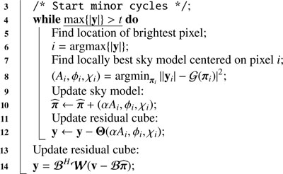
15 Compute model cube:  ;
;
16 Compute restored cube: 
For 2+1D deconvolution, we followed the standard approach for cleaning polarization data, while accounting for DDEs. To achieve approximately the same resolution across the bandwidth, we first applied a sigmoid taper in the uυ-plane, resulting in a resolution of 9.6″ × 9.1″. We used Briggs weighting throughout this work with a robust factor of 0. Although the resolution could be improved for both reconstruction methods by adjusting the weighting scheme, optimizing resolution was not the focus of this work and was not investigated further.
The imaging began with a 2D deconvolution driven by the peak polarized intensity map, |P| defined as
 (19)
(19)
where Qi and Ui denote the linear polarization components at channel i and N is the number of gridding channels. In each minor iteration, the flux corresponding to the brightest pixel in the peak polarized map, scaled by the loop gain, was added to the model cube, while the scaled and shifted spectral PSF was subtracted from the residual image. When the peak flux reached the minor loop threshold, each facet of the model cube was Fourier transformed to data space, where it was compared with the data to compute the next residual. Once the final threshold was reached, each channel of the model cube was convolved with a common restoring beam corresponding to the lowest resolution of the bandwidth. To assess the impact of time-dependent beam effects, we also performed a deconvolution without correcting for beam variations, applying only the mean beam afterward. However, this did not produce significant differences from the previous 2+1D reconstruction, and therefore we do not present these results here.
For RM synthesis, the absolute RM search range was set based on the mean channel width in λ2, resulting in a minimum sensitivity of ~70% at the edges of the sampled Faraday depth. The Faraday depth was sampled at 10 points per full width at half maximum (FWHM) of the RM synthesis dirty beam. We performed RM synthesis and RMCLEAN using the RM-TOOLS package, with a cleaning threshold of 5σQU. Uniform weighting was used for RM synthesis, for both the 2+1D and 3D reconstructions.
The 3D reconstruction was created following the procedure described in Sect. 3. We used RM-TOOLS to perform RM synthesis, as it employs the fast Fourier transform, which significantly accelerated the process. From a Gaussian fit to the real part of the main lobe of the 3D PSF, we obtained a restoring beam FWHM of 8.9″ × 8.6″ × 39.0 rad m−2.
Both deconvolution algorithms were run for a total of ten major iterations, with a maximum of 10 000 minor iterations. We adopted early stopping in the minor cycles, stopping at half the initial peak flux. After deconvolution, we fitted a 3D Gaussian to peaks at the positions of the true signals, using the peak flux and the corresponding RM as initial estimates. The intrinsic polarization angle was recovered by linear interpolation between the adjacent sampling in ϕ. and the flux was corrected for polarization bias following George et al. (2012).
In Fig. 1, we compare the 2+1D and 3D deconvolution algorithms in terms of their ability to recover the input parameters. Detections with a signal-to-noise ratio below four are excluded from the plot to minimize false positives. Both methods successfully recovered the input RM, with no significant difference between them. The 3D reconstruction shows an accurate recovery of the flux across the dynamic range, with no significant correlation with the input RM. In contrast, the 2+1D deconvolution systematically underestimates the flux of high-RM components due to bandwidth depolarization, as indicated by the marker sizes in the figure. Regarding the polarization angle, both methods show errors centered on zero, with mean absolute errors of 3.2° and 3.4° for the 2+1D and 3D algorithms, respectively.
Fig. 2 provides a clearer view of the bandwidth depolarization effect of channel averaging. When bandwidth depolarization is not corrected for, the recovered flux exhibits a systematic trend with Faraday depth. The 2+1D method underestimates flux at high Faraday depths, while the bandwidth-corrected 3D reconstruction yields errors that are generally centered around zero. The error bars tend to increase as a function of |φ|, due to the lower signal-to-noise ratio at lower sensitivities. In Appendix A we attempt to correct the 2+1D reconstruction for bandwidth depolarization, using a tool from the RM-TOOLS package.
To evaluate the performance of the two deconvolution methods independently of the bandwidth depolarization correction, we examined the flux distribution in the residual spectral cube (Fig. 3). The 2+1D reconstruction shows a clear shift in the peak position of the distribution, indicating a higher residual root mean square. Additionally, the presence of higher flux values is a result of the shallower deconvolution, leaving more signal flux in the residuals.
Table 2 lists the run times of the 2+1D and 3D imaging techniques. Both algorithms were executed on an AMD EPYC 7H12 CPU, running at a clock frequency of 2.6 GHz, using up to 128 threads for parallelization and a maximum of 500 GB of memory. The main bottleneck of the 3D deconvolution was the degridding step onto the larger set of frequency channels. The minor iterations contributed only a small fraction of the total runtime. As a result, although the 2+1D deconvolution required more iterations, this did not significantly impact its total runtime. Summing the run times of the 2+1D method, the total was longer than for the 3D method. The 3D deconvolution can be further accelerated by reducing the number of degridding channels, at the cost of less accurate bandwidth depolarization correction.
Observation configuration of synthetic MeerKAT data.
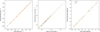 |
Fig. 1 Reconstructed source parameters compared to the input of the synthetic MeerKAT dataset. Blue dots denote the 2+1D reconstruction while orange crosses denote the 3D reconstruction. Left: true vs. recovered RM. Middle: true vs. recovered flux. Right: true vs. recovered intrinsic polarization angle. Marker sizes are proportional to the absolute RM. |
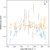 |
Fig. 2 Comparison of the 2+lD (blue) and 3D (orange) methods for the effects of bandwidth depolarization. Only signals with a signal-to-noise above 8σQU are shown. |
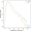 |
Fig. 3 Flux distribution in the residual spectral cube for the 2+1D (blue) and 3D (orange) deconvolution methods. |
Runtimes on synthetic MeerKAT data.
Observation configuration of LOFAR data.
5 LOFAR observation
In this section, we apply our implementation of the 3D imaging technique to a LOFAR HBA pointing from LoTSS DR2 (Shimwell et al. 2022). From the catalog of polarized sources produced by O’Sullivan et al. (2023) (hereafter referred to as OS23), we selected the region with the highest density of polarized sources per square degree and used the corresponding pointing for our analysis. The imaging configuration of the dataset is shown in Table 3. We used the full frequency resolution in both image and data space, resulting in a maximum observable Faraday depth of ± 170 rad m−2 at full sensitivity and ±450 rad m−2 at 50% sensitivity. We used the same sampling as OS23, with a maximum Faraday depth of ±120 rad m−2 and a sampling of 0.05 rad m−2, yielding 4801 samples in φ. As our goal was to produce a polarized intensity map and an RM map, we used the RMSYNTH3D function from RM-TOOLS for 2+1D RM synthesis. Due to the varying noise level across the field, as a consequence of the primary beam correction, a 3D noise map would be required to use the inverse-variance weighting. Since this functionality is not yet implemented in either RM-TOOLS or our software, we instead applied uniform weighting for RM synthesis. An attempt was made to taper the visibilities for the 2+1D method, but this introduced severe artifacts that were not removed during deconvolution. Instead, we applied a common restoring beam, set by the lowest frequency, with a resolution of 7.42″. Although the 3D method achieved a higher resolution of 6.31″, we used the same restoring beam as in the 2+1D approach to enable a direct comparison between the resulting polarized intensity images. As we were using the same frequency resolution in image space as in data space, we did not apply any correction for bandwidth depolarization. We divided the FOV into 7 × 7 facets and applied the direction-dependent calibration solutions, as well as the primary beam correction, during imaging. Due to the higher sampling in φ, we ran the code on a high-memory computing cluster, on a single node with 3 TB of available RAM.
Figure 4 presents a zoom-in on the polarized sources detected by OS23, comparing the 2+1D and 3D deconvolution methods. Although the sources were recorded as six separate entries in the catalog, we identified four as originating from the same double-lobed galaxy. The most notable difference between the reconstructions is the presence of artifacts around bright sources in the 2+1D case, which are largely absent in the 3D reconstruction. The presence of bright Stokes I sources within the FOV introduces leakage into the linear polarization components, delaying the deconvolution of polarized sources until later stages. The 2+1D method struggles to recover faint emission near the noise level, which leads to incomplete deconvolution of the sources shown here. Although the flux appears brighter in the 2+1D image, this can be attributed to undeconvolved extended emission, which also leads to smoother emission and blends small-scale structures. In contrast, the 3D reconstruction better preserves compact features and reduces contamination from sidelobes, resulting in a more accurate representation of the underlying source structure. We do not observe a significant difference in noise levels between the reconstructions, as both images have a σQU of 45 µJy beam−1 in source-free regions.
Figure 5 shows the RM maps from the 2+1D and 3D reconstructions. The RM is obtained from a Gaussian fit to the peaks above 5.5 σQU in the Faraday cube. Only pixels with flux above 8σQU, after correcting for polarization bias, are included in the final RM map. While the 2+1D recovers more flux above the 8σQU level, some of the artifacts around the compact sources also exceed this level, resulting in false detections. In contrast, with the 3D approach, we can lower the detection threshold to 6.5σQU without introducing spurious detections. However, since this would not be a fair comparison, we do not include it here. For the 3D reconstruction, we find that all sources found by OS23 are above the 8σQU level, although some exhibit a slight positional shift, likely due to the different resolution.
Table 4 compares the recovered RMs from the two reconstructions with those reported by OS23. We computed the RM from a Gaussian fit to the highest peak in φ, located at the positions recorded by OS23. The errors were calculated in the standard manner, as the FWHM of the PSF in φ divided by twice the signal-to-noise ratio. We did not compare the Galactic RM-corrected values, as the correction procedure would be identical for both our work and that of OS23, adding no additional information.
We find that only one RM value from the 3D reconstruction is consistent with those reported in OS23. The discrepancy between the values is not unexpected given the differences in resolutionb - both spatially and in φ - as OS23 applies inverse-variance weighting in frequency, while we weighted each channel uniformly. The 2+1D reconstruction generally agrees more with OS23, with the exception of one source (9h28m22s, +41°42′22″), which, as shown in Fig. 5, is significantly contaminated by artifacts. Furthermore, the RM is close to the Stokes I leakage at φ = 0, potentially causing the shift to a lower recovered RM. We also compared the flux densities with those from OS23. The fluxes from OS23 are systematically higher than those in our study, likely because the larger beam size integrates over a broader region, capturing more extended emission. Furthermore, the positions are slightly shifted from those identified in the 2+1D and 3D approaches due to differences in resolution. Although shifting to the positions detected by our method increases the peak flux, the resulting RM values do not align more closely with those reported by OS23.
Figure 6 shows a polarized source not detected by OS23. The source is located 0.75° west of the sources in Fig. 4 and, from the Stokes I image, appears to be a double-lobed galaxy. However, only one of the lobes is detected in polarized emission outside the Stokes I leakage range. From a Gaussian fit to the main peak, we obtain an RM of −6.20 + 0.05, in contrast to the positive RMs of the other sources in the field. Whether this difference arises due to foreground Faraday rotation, intrinsic properties of the source, or its surroundings requires further analysis. Since OS23 determines the noise level from the wings of the dirty Faraday dispersion (|φ| > 100 rad m−2), it is likely an overestimate of the noise, particularly for bright or high-RM sources. This could explain why their search algorithm does not detect this source.
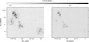 |
Fig. 4 Polarized source reconstructions using 2+1D (left) and 3D (right) methods. Red circles mark six polarized sources from OS23. The 2+1D reconstruction contains significant artifacts around the northern lobe and isolated unresolved sources. |
Comparison of the RM and flux values obtained from the two reconstruction methods for the six polarized sources identified in OS23.
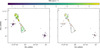 |
Fig. 5 Rotation measure maps from the 2+1D (left) and 3D (right) reconstructions, centered on the six polarized sources from OS23, indicated as red circles. Only pixels with a flux higher than 8σQU are shown. The Stokes I 10σI noise level is shown as a black contour. |
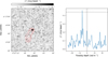 |
Fig. 6 Polarized source previously not detected by OS23, found using our 3D reconstruction method. Left: polarized intensity map centered on the source. The Stokes I (10, 20, 50) × σI noise levels are shown as red contours. Right: magnitude of the LOS profile at the brightest pixel, with the local 8σQU level shown as a dashed black line. The shaded area indicates the range of Stokes I leakage between −1 and 1 rad m−2. |
6 Discussion
Since the 2+1D deconvolution is driven by the mean flux map from the entire bandwidth, rather than convolving a series of Stokes Q and U images, we do not observe the same source flux underestimation as reported in Bell & Enßlin (2012), where the reconstruction of low-flux sources was limited by the noise in individual frequency channels. Instead, the observed bias in Fig. 1 is not dependent on source flux, but rather on the input RM, as a result of bandwidth depolarization. Correcting for bandwidth depolarization could, in principle, be applied to the 2+1D reconstruction. However, such a correction would require additional information that is typically not well known after deconvolution, making it more of an approximation than a reliable recovery of the true depolarization. As these corrections are not widely implemented to our knowledge, our main comparison in Sect. 5 does not apply such a correction. However, in Appendix A, we evaluate the accuracy of the adjoint transform correction, as presented in Fine et al. (2023).
Our 3D reconstruction inherently accounts for the effects of channel averaging during imaging, incorporates flagged channel information, and the mapping between frequency resolutions to determine their relative bandwidth depolarization. This approach becomes particularly advantageous in the later stages of deconvolution, where false positives amplified by the correction are naturally corrected in the major cycle. This correction can only be applied if the frequency resolution of the data is higher than that of the image products. In the case of a LOFAR observation, where essentially full frequency resolution is required to achieve high sensitivity at high Faraday depths, alternative approaches must be used, such as those presented by Fine et al. (2023).
While the improvements achieved by our reconstruction technique for simulated unresolved sources arise primarily from bandwidth depolarization correction rather than Faraday synthesis alone, its true advantages become evident for spatially resolved structures, as shown in Fig. 4. The large number of degrees of freedom ( ) in the 2+1D reconstruction leads to overfitting of the true source flux, allowing noise and artifacts from the PSF of nearby pixels to be incorporated into the model. In contrast, the 3D reconstruction is parametrized only by the Gaussian fit parameters and the intrinsic polarization angle of the source, enabling a more stable, faster, and deeper deconvolution. This deeper deconvolution improves the accuracy of polarized emission reconstruction and increases the dynamic range, potentially enhancing RM grid densities by detecting more polarized sources.
Following Bell & Enßlin (2012), we assumed that Faraday synthesis eliminates the need for resolution matching, as spectral variations in resolution across the bandwidth are inherently accounted for in the 3D PSF. However, this assumption is only valid if the source structure can be well approximated by a single point, as assumed in the CLEAN algorithm. If this condition is not met, resolution matching remains necessary unless the magnetic field is ordered and the RM is approximately constant within the beam area. Otherwise, frequency-dependent beam depolarization occurs due to the varying resolution, which is not modeled by the 3D PSF. As our implementation of Faraday synthesis used the CLEAN algorithm for deconvolution, we assumed that the first condition was met, and thus did not perform resolution matching. However, for sources with extended emission or complex Faraday dispersions, this assumption may lead to inaccuracies due to unmodeled frequency-dependent beam depolarization. Future studies should investigate how such effects influence the reconstruction of Faraday dispersions and whether incorporating resolution matching into the deconvolution process improves accuracy.
Furthermore, the 3D PSF constructed in this work assumes a flat spectrum across the bandwidth. In contrast, a common approach in RM synthesis is to account for the spectral dependence by either applying a spectral index correction or performing RM synthesis on the fractional polarizations,
 (20)
(20)
where  is the modeled Stokes I flux, excluding noise. However, since DDFACET jointly deconvolves all Stokes parameters, this correction cannot be applied within the current framework. Future work will explore the incorporation of a user-defined spectral index across the entire field, which may improve RM recovery for sources with steep spectra.
The main challenge of Faraday synthesis is the high memory demand associated with large transformations. In particular, the Fourier transform from λ2 to φ is the most computationally expensive step, making it impractical for large fields of view and high-spectral-resolution data. As a result, the LOFAR example presented in this work was limited to a field of view of 1° × 1°, as larger images would have exceeded memory constraints, even with 3 TB of available RAM. Memory usage can be reduced by, for example, computing only a small patch of the PSF in φ, similar to typical CLEAN practice. While DDFACET generally processes each facet in parallel, memory-intensive operations can be run sequentially, though at a significant cost in computation time. Most computational time for LOFAR polarization deconvolution is spent on deconvolving polarization leakage, characterized by a peak around φ = 0. Future studies will explore the possibility of excluding this leakage range, as it does not contribute to scientific analysis and would otherwise be blanked, as in OS23. This would significantly reduce the computation time for LOFAR data, as only a fraction of the current number of minor iterations would be necessary for a given deconvolution threshold.
One potential application for direction-dependent Faraday synthesis is the International LOFAR Two-metre Sky Survey4 (ILoTSS), which will deliver high-resolution (0.3″) data products of radio sources across the northern sky. To accurately analyze these data, polarization deconvolution will be essential for a correct recovery of the RMs and magnetic field structure in these well-resolved sources with complex magnetoionic environments.
While the MeerKAT L-band offers a spatial resolution comparable to that of LoTSS, its channel width in λ2 is significantly narrower. This results in a much higher maximum observable Faraday depth, given by
 (21)
(21)
for a given number of frequency channels. Consequently, only a few tens of channels are needed to achieve sensitivity to Faraday depths relevant to most cosmic magnetism studies. With access to high-memory computing clusters, Faraday synthesis could also be applied to ASKAP cosmic magnetism studies (POSSUM; Vanderwoude et al. 2024), potentially increasing the RM grid density. Combined with the bandwidth depolarization correction implemented in this work, Faraday synthesis becomes a viable approach for high-resolution polarization imaging.
7 Conclusions
We have incorporated Faraday synthesis into DDFACET, a modern radio imaging tool designed for wide-field, wide-band interferometric imaging. Additionally, we have introduced a novel implementation of a direction-dependent Faraday synthesis deconvolution algorithm, and tested the algorithm on both synthetic data, modeled on MeerKAT observations, and observational data from LOFAR. The 3D deconvolution method shows a significant reduction in artifacts, while increasing both the dynamic range and resolution. Although our Faraday synthesis algorithm requires more memory, it achieves faster runtimes compared to the 2+1D approach. Our method has led to the detection of a previously unidentified polarized source. Our bandwidth depolarization correction has been shown to accurately recover the intrinsic flux of depolarized sources, allowing us to image polarization data at a coarser frequency resolution while still maintaining high sensitivity at large Faraday depths. Future interferometers, such as MeerKAT+ and eventually the SKA, will require direction-dependent imaging to account for variations between antennas. In this context, direction-dependent Faraday synthesis is a promising approach for polarization studies. The code implementing this method will be made publicly available shortly after the publication of this paper as part of the DDFACET repository5.
Acknowledgements
VG acknowledges support by the German Federal Ministry of Education and Research (BMBF) under grant D-MeerKAT III. MB acknowledges funding by the Deutsche Forschungsgemeinschaft (DFG, German Research Foundation) under Germany’s Excellence Strategy – EXC 2121 “Quantum Universe” – 390833306 and the DFG research unit “Relativistic Jets”. SPO acknowledges support from the Comunidad de Madrid Atracción de Talento program via grant 2022-T1/TIC-23797, and grant PID2023-146372OB-I00 funded by MICIU/AEI/10.13039/501100011033 and by ERDF, EU. FdG acknowledges support from the ERC Consolidator Grant ULU 101086378. We acknowledge data storage and computational facilities by the University of Bielefeld which are hosted by the Forschungszentrum Jülich and that were funded by German Federal Ministry of Education and Research (BMBF) projects D-LOFAR IV (05A17PBA) and D-MeerKAT-II (05A20PBA), as well as technical and operational support by BMBF projects D-LOFAR 2.0 (05A20PB1) and D-LOFAR-ERIC (05A23PB1), and German Research Foundation (DFG) project PUNCH4NFDI (460248186). We thank the anonymous referee for their constructive comments and suggestions, which have helped to improve the manuscript.
Appendix A Bandwidth depolarization
Bandwidth depolarization arises from the finite bandwidth of frequency channels, leading to signal averaging within each bin. This effect is visible as a function of |φ|, where rapid Faraday rotation within a channel causes partial cancellation of Stokes Q and U, reducing the observed polarization.
With our 3D deconvolution method, correcting for bandwidth depolarization is a requirement rather than an optional improvement, as neglecting it would leave significant residuals in the major cycle, preventing proper convergence. This is due to the different frequency resolutions in image space and data space, where less depolarization is experienced in the higher resolution data space. The approach is analogous to the time-dependent beam correction in DDFACET: while the residual image represents the time-averaged sky brightness distribution, the forward step applies time-dependent beam Jones matrices to ensure consistency with the visibility data. However, our correction does not require a facet-based approach, as the number of data points in φ is significantly smaller than the number of pixels in image space. Instead, we compute the correction by simulating channel averaging from degridding to gridding frequencies on synthetic samples with an RM corresponding to each sampled point in φ. By performing RM synthesis on each sample and comparing the output flux to the input, we obtain a correction factor as a function of |φ|.
In an attempt to correct the 2+1D reconstruction for bandwidth depolarization, we used the bwdepol module within RM-TOOLS. The depolarization estimate is produced using the adjoint transform, discussed in Fine et al. (2023). Before we fit a Gaussian to the peaks in the deconvolved Faraday cubes, we divide the Faraday dispersion by the sensitivity estimate. The results are seen in Fig. A.1. We see that the correction is an overestimate of the true depolarization, as the errors appear to increase as a function of |φ|.
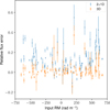 |
Fig. A.1 A comparison between the bandwidth depolarization corrected 2+1D (blue) and 3D (orange) methods on the effects of bandwidth depolarization. Only signals with a signal to noise above 8σQU are included in the figure. |
References
- Anderson, C. S., McClure-Griffiths, N. M., Rudnick, L., et al. 2024, MNRAS, 533, 4068 [NASA ADS] [CrossRef] [Google Scholar]
- Bell, M. R., & Enßlin, T. A. 2012, A&A, 540, A80 [NASA ADS] [CrossRef] [EDP Sciences] [Google Scholar]
- Böckmann, K., Brüggen, M., Heesen, V., et al. 2023, A&A, 678, A56 [NASA ADS] [CrossRef] [EDP Sciences] [Google Scholar]
- Brentjens, M. A., & de Bruyn, A. G. 2005, A&A, 441, 1217 [Google Scholar]
- Burn, B. J. 1966, MNRAS, 133, 67 [Google Scholar]
- Clark, B. G. 1980, A&A, 89, 377 [Google Scholar]
- de Gasperin, F., Rudnick, L., Finoguenov, A., et al. 2022, A&A, 659, A146 [NASA ADS] [CrossRef] [EDP Sciences] [Google Scholar]
- De Rubeis, E., Stuardi, C., Bonafede, A., et al. 2024, A&A, 691, A23 [NASA ADS] [CrossRef] [EDP Sciences] [Google Scholar]
- Fine, M. A., Van Eck, C. L., & Pratley, L. 2023, MNRAS, 520, 4822 [Google Scholar]
- George, S. J., Stil, J. M., & Keller, B. W. 2012, PASA, 29, 214 [Google Scholar]
- Högbom, J. A. 1974, A&AS, 15, 417 [Google Scholar]
- Jonas, J., & MeerKAT Team 2016, in MeerKAT Science: On the Pathway to the SKA, 1 [Google Scholar]
- Offringa, A. R., & Smirnov, O. 2017, MNRAS, 471, 301 [Google Scholar]
- O’Sullivan, S. P., Shimwell, T. W., Hardcastle, M. J., et al. 2023, MNRAS, 519, 5723 [CrossRef] [Google Scholar]
- Perley, R. A., Chandler, C. J., Butler, B. J., & Wrobel, J. M. 2011, ApJ, 739, L1 [Google Scholar]
- Shimwell, T. W., Hardcastle, M. J., Tasse, C., et al. 2022, A&A, 659, A1 [NASA ADS] [CrossRef] [EDP Sciences] [Google Scholar]
- Smirnov, O. M. 2011, A&A, 527, A106 [NASA ADS] [CrossRef] [EDP Sciences] [Google Scholar]
- Tasse, C., Hugo, B., Mirmont, M., et al. 2018, A&A, 611, A87 [NASA ADS] [CrossRef] [EDP Sciences] [Google Scholar]
- Vanderwoude, S., West, J. L., Gaensler, B. M., et al. 2024, AJ, 167, 226 [CrossRef] [Google Scholar]
- van Haarlem, M. P., Wise, M. W., Gunst, A. W., et al. 2013, A&A, 556, A2 [NASA ADS] [CrossRef] [EDP Sciences] [Google Scholar]
- van Weeren, R. J., Williams, W. L., Hardcastle, M. J., et al. 2016, ApJS, 223, 2 [Google Scholar]
As the linear Stokes vectors only yields the (RL, LR) circular correlations, we use the linear correlations in this paper.
The beam effects were simulated using https://github.com/ratt-ru/eidos?tab=readme-ov-file
All Tables
Comparison of the RM and flux values obtained from the two reconstruction methods for the six polarized sources identified in OS23.
All Figures
|
Fig. 1 Reconstructed source parameters compared to the input of the synthetic MeerKAT dataset. Blue dots denote the 2+1D reconstruction while orange crosses denote the 3D reconstruction. Left: true vs. recovered RM. Middle: true vs. recovered flux. Right: true vs. recovered intrinsic polarization angle. Marker sizes are proportional to the absolute RM. |
| In the text | |
|
Fig. 2 Comparison of the 2+lD (blue) and 3D (orange) methods for the effects of bandwidth depolarization. Only signals with a signal-to-noise above 8σQU are shown. |
| In the text | |
|
Fig. 3 Flux distribution in the residual spectral cube for the 2+1D (blue) and 3D (orange) deconvolution methods. |
| In the text | |
|
Fig. 4 Polarized source reconstructions using 2+1D (left) and 3D (right) methods. Red circles mark six polarized sources from OS23. The 2+1D reconstruction contains significant artifacts around the northern lobe and isolated unresolved sources. |
| In the text | |
|
Fig. 5 Rotation measure maps from the 2+1D (left) and 3D (right) reconstructions, centered on the six polarized sources from OS23, indicated as red circles. Only pixels with a flux higher than 8σQU are shown. The Stokes I 10σI noise level is shown as a black contour. |
| In the text | |
|
Fig. 6 Polarized source previously not detected by OS23, found using our 3D reconstruction method. Left: polarized intensity map centered on the source. The Stokes I (10, 20, 50) × σI noise levels are shown as red contours. Right: magnitude of the LOS profile at the brightest pixel, with the local 8σQU level shown as a dashed black line. The shaded area indicates the range of Stokes I leakage between −1 and 1 rad m−2. |
| In the text | |
|
Fig. A.1 A comparison between the bandwidth depolarization corrected 2+1D (blue) and 3D (orange) methods on the effects of bandwidth depolarization. Only signals with a signal to noise above 8σQU are included in the figure. |
| In the text | |
Current usage metrics show cumulative count of Article Views (full-text article views including HTML views, PDF and ePub downloads, according to the available data) and Abstracts Views on Vision4Press platform.
Data correspond to usage on the plateform after 2015. The current usage metrics is available 48-96 hours after online publication and is updated daily on week days.
Initial download of the metrics may take a while.