| Issue |
A&A
Volume 700, August 2025
|
|
|---|---|---|
| Article Number | A207 | |
| Number of page(s) | 11 | |
| Section | Cosmology (including clusters of galaxies) | |
| DOI | https://doi.org/10.1051/0004-6361/202555018 | |
| Published online | 20 August 2025 | |
Individual halo bias in models of f(R) gravity
1
Departamento de Física, Universidad de Córdoba, E-14071 Córdoba, Spain
2
Departamento de Física, Universidad Técnica Federico Santa María, Avenida Vicuña Mackenna 3939, San Joaquín, Santiago, Chile
3
Instituto de Astrofísica de Canarias, s/n, E-38205 La Laguna, Tenerife, Spain
4
Departamento de Astrofísica, Universidad de La Laguna, E-38206 La Laguna, Tenerife, Spain
⋆ Corresponding author: This email address is being protected from spambots. You need JavaScript enabled to view it.
Received:
3
April
2025
Accepted:
11
July
2025
Abstract
Context. Halo bias links the statistical properties of the spatial distribution of dark matter (DM) halos to those of the underlying DM field, providing insights into clustering properties in both general relativity (GR) and modified-gravity such as f(R) models. While the primary halo mass-dependent bias has been studied in detailed, the secondary bias, which accounts for the additional dependencies on other internal halo properties, can offer a sensitive probe for testing gravity beyond the Λ-cold dark matter (ΛCDM) model.
Aims. The aim of this study is to quantify any potential deviations between ΛCDM and f(R) gravity models in halo clustering, at both the primary and secondary level, as well as in the distributions of halo properties in the cosmic web.
Methods. Using N-body simulations of f(R) gravity models, we assessed the scaling relations and the primary and secondary bias signals of halo populations on the basis of a halo-by-halo estimator of large-scale effective bias. Our analysis was performed using halo number density as the independent variable.
Results. The relative difference in the effective bias between the f(R) models and ΛCDM is sensitive, albeit slightly, to the power index of modified gravity. The largest deviations from GR are measured for low-mass halos, where the average bias at a fixed number density decreases by up to 5% for fixed scaling indices. We also show that the scaling relations for some environmental properties, including neighbour statistics, Mach number, and local overdensity, exhibit small but non-negligible deviations (3–5%) from GR for a wide range of number densities. Our results suggest that the properties of halos in sheets and voids show the largest departures from GR (> 10% in some cases). In terms of secondary bias, we do not find any statistically significant deviations with respect to ΛCDM for any of the properties explored in this work.
Key words: methods: numerical / galaxies: halos / large-scale structure of Universe
© The Authors 2025
 Open Access article, published by EDP Sciences, under the terms of the Creative Commons Attribution License (https://creativecommons.org/licenses/by/4.0), which permits unrestricted use, distribution, and reproduction in any medium, provided the original work is properly cited.
This article is published in open access under the Subscribe to Open model. This email address is being protected from spambots. You need JavaScript enabled to view it. to support open access publication.
1. Introduction
The physical origin of the late-time accelerated expansion of the Universe remains one of the most pressing open problems in modern cosmology. This challenge is further compounded by the latest cosmological constraints from the Dark Energy Spectroscopic Instrument (DESI) (DESI Collaboration 2025). Cosmic acceleration can potentially be explained through two primary avenues: either by invoking dark energy models characterised by an equation of state that generates a negative pressure, possibly with a time-dependent variation, or alternatively by modifying general relativity (GR), a framework that remains largely untested on cosmological scales.
Recent studies show that while modified gravity (MG) does not unequivocally outperform the standard ΛCDM model, it offers a robust physical mechanism for safely crossing the phantom divide (see, e.g. Bamba et al. 2008; de Haro et al. 2023; Odintsov et al. 2024). This is investigated in the context of the general scalar-tensor Horndeski theory, a MG framework that encompasses the widely studied f(R) theory (see, e.g. Chudaykin & Kunz 2024). The f(R) models, extensively explored in the literature (for a concise review see Koyama 2016; Nojiri et al. 2017), are of particular interest because they represent a minimal yet significant modification of GR. A family of f(R) models, including the popular Hu & Sawicki (2007) parametrisation, in light of DESI data, has also been tested alongside other cosmological data (Ishak et al. 2024; Plaza & Kraiselburd 2025). At the same time, forecasts from the Euclid space mission (Laureijs et al. 2011) suggest that it will be capable of distinguishing f(R) gravity from the ΛCDM model with a confidence level exceeding 3σ by combining spectroscopic and photometric probes (Casas et al. 2023; Frusciante et al. 2024). Additional insights into f(R) gravity, derived from the full-shape galaxy power spectrum, are discussed in Aviles (2025).
Beyond its potential to explain cosmic acceleration and provide an accurate description of cosmic microwave background observations and galaxy clustering (Berti et al. 2015), f(R) gravity presents a compelling alternative to dark energy models by preserving the source tensor while introducing modifications to the field equations themselves. Plausible modifications of gravity employ a screening mechanism that suppresses the effect of the fifth force in regimes where strong constraints on gravity are set by observations, such as the Solar System. In this study, we consider the Hu & Sawicki (2007) parametrisation of f(R), combined with a screening mechanism as described by Khoury & Weltman (2004). In this framework, the modification of gravity manifests as the addition of a scalar field coupled to matter, which introduces changes in the density field. As a result, deviations from GR are expected to appear in the clustering properties of biased cosmic tracers, such as galaxies, DM halos, and quasars. A variety of approaches have been employed with the aim of distinguishing potential variations in gravity from the standard ΛCDM model, with efforts including the study of redshift-space distortions (Jennings et al. 2012; Wright et al. 2019; García-Farieta et al. 2019, 2020; Hernández-Aguayo et al. 2019; Fiorini et al. 2022; Liu et al. 2025), tracer bias and sample selection (Arnalte-Mur et al. 2017; García-Farieta et al. 2021), the bispectrum of lensing (Chudaykin et al. 2025) and matter (Gil-Marín et al. 2011), cosmic voids (Zivick et al. 2015; Voivodic et al. 2017; Perico & Tamayo 2017; Contarini et al. 2021), halo mass functions (Hagstotz et al. 2019; Gupta et al. 2022), weak-lensing statistics (Peel et al. 2018; Giocoli et al. 2018; Maggiore et al. 2025) and a variety of complementary methodologies such as (Peel et al. 2019) and (Corasaniti et al. 2020).
In this work, we investigate the effect of assuming different f(R) models on the linear bias of DM halos, focusing on its multiple dependencies. The term secondary halo bias is used to represent all dependencies of halo bias that are measured at a fixed halo mass; the dependence of bias on halo (virial) mass is considered here the primary dependence, arising from the fundamental connection between bias and the peak height of density fluctuations (see, e.g. Kaiser 1984; Bardeen et al. 1986; Mo & White 1996; Sheth & Tormen 1999; Sheth et al. 2001; Tinker et al. 2010). Secondary bias have been measured for a large number of internal halo properties, including concentration, formation time, shape or spin, to name but a few1 (see, e.g. Sheth & Tormen 2004; Gao et al. 2005; Wechsler et al. 2006; Gao & White 2007; Dalal et al. 2008; Angulo et al. 2008; Li et al. 2008; Faltenbacher & White 2010; Lazeyras et al. 2017; Salcedo et al. 2018; Mao et al. 2018; Han et al. 2019; Sato-Polito et al. 2019; Johnson et al. 2019; Ramakrishnan et al. 2019; Contreras et al. 2019; Montero-Dorta et al. 2020, 2021, 2025; Tucci et al. 2021; Contreras et al. 2021b; Balaguera-Antolínez et al. 2024; Montero-Dorta & Rodriguez 2024).
At a fixed halo mass, the bias also correlates with the properties of the environment that halos inhabit, including the local overdensity, the anisotropy of the tidal field, the distance to cosmic-web features, or even the Mach number (e.g. Paranjape et al. 2018; Montero-Dorta & Rodriguez 2024; Balaguera-Antolínez et al. 2024). The significance of some of these environmental properties resides in the fact that they can be seen as mediators linking bias and the internal properties of halos (Paranjape et al. 2018; Ramakrishnan et al. 2019). In Balaguera-Antolínez et al. (2024), we analysed the secondary bias signals produced by a variety of internal and environmental properties, along with the dependence of the trends on the location of halos within the cosmic web.
To facilitate the analysis of bias for different f(R) models, we use a halo-by-halo bias estimator (Paranjape et al. 2018; Contreras et al. 2021a; Balaguera-Antolínez et al. 2024; Montero-Dorta et al. 2025), which provides significant analytical advantages as compared to the traditional approach based on ratios of correlation functions or power spectra (see Balaguera-Antolínez et al. 2024 for more information).
The outline of this paper is as follows. In Sect. 2, we briefly describe the background theory, summarising the modified gravity model we consider and describing our set of simulations. Section 3 details the method used to assign the individual effective halo bias and its application to the f(R) simulations. The results of the effective bias, as well as the primary and secondary bias relations measured in the f(R) halo catalogues, are presented in Sect. 4. Finally, in Sect. 5, we summarise our main findings and discuss the implications of our results.
2. Models and simulations
The f(R) theory of gravity is a notable example of a non-standard cosmological model developed to address some of the issues present in the ΛCDM model (see Clifton et al. 2012; Sotiriou & Faraoni 2010, for in-depth details). Among the various parametrisations of this theory, the Hu & Sawicki (2007) one is particularly well studied due to its physical motivation and the fact that it remains a viable model, not yet ruled out by observations (Aviles 2025; Dainotti et al. 2025; Liu et al. 2016; Landim et al. 2024; Artis et al. 2024; Vogt et al. 2025). This model modifies the Einstein-Hilbert action by replacing the Ricci scalar with a function, f(R), such that R ↦ R + f(R). The function, f(R) can be adjusted to match, to first order, the background expansion of the ΛCDM model and, for the Hu-Sawicki parametrisation, it is modelled as a broken power law of the Ricci scalar, given by
 (1)
(1)
where Λ and μ2 serve as free parameters for each value of the power index, n. In the limit of small deviations from GR, i.e., R ≫ μ, the f(R) function is approximately equal to
 (2)
(2)
where R0 denotes the background Ricci scalar at the current epoch and fR0 is the derivative of f(R) with respect to R (i.e.,  ) evaluated at the present time. This dynamical degree of freedom is typically interpreted as a scalar field and can be approximated as fR0 = −2nΛμ2n/R0n + 1. Note that if |fR0|→0, the boundary condition f(R)→ − 2Λ is satisfied as a consequence of requiring equivalence with ΛCDM. We recall that here n ≥ 0 is an integer, and while most past simulations in f(R) have focused on the scenario where n = 1, the scenario with n = 2 has not been as thoroughly investigated. This paper examines both scenarios within its set of simulations, comparing the results against the standard ΛCDM model.
We used the MG simulation suite described in García-Farieta et al. (2024), which consists of a set of seven high-resolution COLA simulations performed with the FML-COLA solver2. The simulations are consistent with the best-fit parameters of Planck 2018 cosmology: Ωm = 0.311, Ωcdm = 0.2621, Ωb = 0.0489, h = 0.6766, ns = 0.9665, and As = 2.105 × 10⁻⁹ (Planck Collaboration VI 2020). They feature the dynamics of 20483 DM particles in a comoving box of 1 h−1Gpc on each side. The simulations are started at redshift z = 99, at which time non-linear effects are negligible, and evolved up to redshift z = 0.5 using 100 time steps. All the MG models use the same initial conditions as ΛCDM, which were generated using the 2LPTic code (Scoccimarro 1998; Crocce et al. 2006) implemented in FML-COLA. This set-up achieves a mass resolution of Mp = 1.005 × 10¹⁰ h−1 M⊙, ensuring sufficient detail for accurate halo identification. We use the ROCKSTAR halo-finding algorithm (Behroozi et al. 2013) to identify halos in the simulation containing at least 80 DM particles each. To mitigate the small-scale uncertainty of COLA, we adjusted the force resolution in the ROCKSTAR parameter file to be close to the grid size of the simulations. To focus on more massive structures, we applied an additional mass threshold of 1012 h−1 M⊙, retaining only halos exceeding this limit. For our analysis, we considered only the MG models that are not completely ruled out by current constraints, leaving us with four models: (|fR0|, n)∈{(10−5, 1), (10−6, 1), (10−5, 2), (10−6.5, 2)}, which are denoted as {F51, F61, F52, F6.52}.
3. Assignment of individual effective bias
We implemented the approach of Paranjape et al. (2018), in which large-scale (or effective) bias can be assigned to individual tracers in a simulation. This approach implements the estimator for large-scale bias based on the cross-correlation between the halo tracer field and its underlying DM density field (see e.g. Smith et al. 2007; Pollack et al. 2012; Balaguera-Antolínez 2014). Briefly, for a DM tracer at position ri, we assigned individual bias as3
 (3)
(3)
where δdm(k) is the Fourier transform of the underlying DM density field, Pdm(kj) its power spectrum and  is the number of Fourier modes in the j-th spherical bin in Fourier space (see e.g. Ramakrishnan et al. 2019; Han et al. 2019; Paranjape & Alam 2020; Contreras et al. 2021a; Balaguera-Antolínez et al. 2024; Balaguera-Antolínez & Montero-Dorta 2024; Montero-Dorta et al. 2025). The sum is carried over the range of wavenumbers kj < kmax in which the ratio between the halo and the DM power spectra is constant4. Balaguera-Antolínez et al. (2024) showed that the effective bias as a function of multiple halo properties, as obtained from standard approaches (for example, measurements of the auto and cross-power halo power spectrum in bins of a that halo property, see e.g. Balaguera-Antolínez (2014), Pollack et al. (2014)), is consistent with the results obtained from Eq. (3) and with known calibrations in the literature, such as the halo bias – mass relation (Tinker et al. 2010, see also Paranjape et al. 2018). This way of assigning bias to objects has also been proven advantageous as a means of including the clustering signal (up to a given scale kmax) in the machinery for assigning halo properties in the context of so-called calibrated methods, as is discussed by Balaguera-Antolínez & Montero-Dorta (2024).
Figure 1 displays maps of the halo effective bias in slices of 12 h−1Mpc thickness, which vary spatially under different MG models, as labelled. The individual halo effective bias was computed using equation Eq. (3) for all the MG models at z = 0.5. A zoomed-in region, representing a portion of 100 × 100 h−2Mpc2, highlights subtle differences that are visible to the naked eye. In particular, MG models tend to alter the clustering of halos compared to the standard ΛCDM model, resulting in sharper or more fragmented structures in some cases. These differences arise from changes in the gravitational dynamics, which influence the formation and distribution of halos.
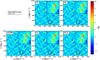 |
Fig. 1. Slices of the ∼12 h−1Mpc thickness in the MG simulations (at z = 0.5) showing the individual bias field. The zoom-in region represents a 100 × 100 h−2Mpc−2 slice. |
4. Results
In this analysis, and to facilitate a fair comparison among the different MG models, we chose to use number density as the independent variable (i.e., the primary halo property) rather than halo mass, as the latter is model-dependent. This choice is motivated by previous research, such as Arnalte-Mur et al. (2017) and García-Farieta et al. (2021), where the clustering statistics of MG models are analysed in terms of halo populations defined by fixing the number density for each catalogue. This approach is essentially a simplified version of halo abundance matching. Figure 2 shows the cumulative halo mass function (HMF)  for the different f(R) models. As is demonstrated by the HMF trend, f(R) models predict a higher number of halos than the ΛCDM model for masses above 1012 h−1 M⊙ due to the enhanced gravitational effects. The zoom-in section of Fig. 2 highlights the intermediate mass range between 1013 and 3 × 10¹³ h−1 M⊙, where all models show slightly different HMF values. As was expected, the F6 family of models closely aligns with ΛCDM, as they exhibit the least gravity enhancement, resulting in a halo mass distribution that resembles that of ΛCDM, with deviations of less than 5%, as shown in the lower panel of Fig. 2. In contrast, the remaining f(R) models, specifically the F5 models, show an excess in halo mass, producing 10–15% more halos than predicted by ΛCDM. As a consequence, the mass cuts corresponding to a given number density vary across the various f(R) catalogues. Therefore, from this point onwards, we present our results in terms of the number density,
  . This choice is made for the sake of a fair comparison among models, and is also motivated by the fact that the virial halo mass is not an observable. Therefore, a sample selection with a fixed Mmin cannot be directly replicated in a real galaxy sample.
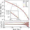 |
Fig. 2. Cumulative halo mass function for the different MG models taken at redshift z = 0.5. The bottom panel shows the relative deviation with respect to the ΛCDM model with lines connecting the data points to guide the eye. |
4.1. Primary bias: scaling relations
We obtained the large-scale halo bias using the object-by-object estimator of Eq. (3), which offers an approach to investigate its dependencies on several halo properties as presented in Balaguera-Antolínez et al. (2024). Figure 3 shows the individual halo effective bias as a function of number density for different f(R) models at z = 0.5. The black points represent the mean bias within a number density bin, with error bars computed as the standard error of the mean for each bin. The colour bar in Fig. 3 represents the number of tracers, Nh, while the contours outline regions with an equal number of tracers. As we see in the figure, the effective bias for the MG models follows a trend similar to that of the baseline ΛCDM model. However, slight differences are observed at low number densities in the f(R) models, mainly due to the large scatter introduced by very massive halos. Notably, models such as F52 and F6.52 exhibit more pronounced shifts and deeper dips, indicating stronger deviations from standard gravity effects at lower number densities ( ).
).
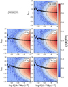 |
Fig. 3. Halo effective bias, bhm, computed at z = 0.5 as a function of the number density. The points denote the mean bias in different mass bins, with errorbars denoting the standard error of the mean. The contours indicate a region of an equal number of tracers Nh. |
In Fig. 4, we compare the relative deviations of the f(R) effective halo bias from ΛCDM, computed as described above, with the shaded bands representing the expected error bars derived from the standard error of the mean halo bias5. As the value of |fR0| increases, the halo bias tends to decrease because halos of a fixed number density become more common and thus less biased. For the F5 models, we observe the effect of the power index on the bias, with visible differences between n = 1 and n = 2. Specifically, for low number densities ( ), no significant impact of the power index is observed, while for
  , we find that F51 is more biased than F52, with a deviation from ΛCDM of about 5% for F51 and approximately 2.5% for F52. In contrast, both F6 models with n = 1 and ones with n = 2 are consistent with ΛCDM within the error bars across the entire number density range, with departures from ΛCDM of up to 2.5%. The impact of the power index in these models is less clear, as they exhibit different amplitudes for the scalaron field |fR0|.
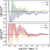 |
Fig. 4. Ratios of the effective halo bias in the f(R) simulations at z = 0.5, measured in bins of the halo viral mass. Symbols denote the mean halo-mass bias ⟨bhm|logMvir⟩. |
In a study on halo statistics, Schmidt et al. (2009) found that in full simulations of f(R) cosmologies – such as the ones in the present work – the difference in bias is reduced compared to simulations that do not account for gravity modifications in the deep potential wells of cosmic structures. According to these findings, the largest deviations from GR for the F51 model occur in low-mass halos (high number density), while for the F61 model, the differences are more noticeable in halos of intermediate mass, rather than in the lowest mass halos. This observation is consistent with the results of our analysis. At background field values of |fR0|≲10−5, current observations show that the enhancement of the gravitational force is suppressed inside halos, significantly reducing the effects on the properties of the most massive halos. Schmidt et al. (2009) pointed out that the scaling relations still have applicability for establishing conservative upper limits on modifications to gravity, even in simpler cases where the halo bias is derived by dividing the halo cross power spectrum by the matter power spectrum. This limitation motivates our approach, which uses the object-by-object bias to set more reliable constraints on modifications to gravity.
We also investigated the behaviour of scaling relations among various halo properties across different simulations, including novel environmental properties introduced by Balaguera-Antolínez et al. (2024), which are based on both the underlying DM field and halo properties. These scaling relations are expected to vary as halos change in mass, or equivalently, as their number density evolves. Differences in the occupancy of the bins of the scaling relations in the f(R) cosmologies can arise through gravitational evolution and the time- and scale-dependence of the growth factor in these models (see e.g. García-Farieta et al. 2024). We assessed the strength of the relationships of the halo scaling relations with secondary properties, as well as their impact on the signal of both the primary and secondary halo bias in these cosmologies. Below, we briefly describe the quantities considered in the scaling relations (for more details, see Balaguera-Antolínez et al. 2024):
-
The maximum circular velocity, Vmax, is defined as Vmax = Max(Vc), where Vc(r) is the Newtonian circular velocity of the halo. Vmax serves as a probe of the potential well of DM halos. Arnold et al. (2016) showed, using zoomed-in simulations of Milky Way-like halos in f(R) cosmologies, that the gravitational potential drops below a crucial threshold for halos with masses greater than 2.3 × 10¹² h−1M⊙. This results in a rapid suppression of the fifth force of MG, leading to significant deviations from the ΛCDM model. However, at a close radius of r200 (the radius that encloses a sphere with a mean density 200 times the critical density), Vmax tends to remain unchanged relative to ΛCDM due to the screening mechanism of MG.
-
The halo ellipticity, denoted as ℰh, measures the shape of the halo and is defined as the ratio of the semi-axes a, b, and c of the halo’s ellipsoid, given by
 , where q = b/a and s = c/a, with the condition a > b > c. The semi-axes, a, b, and c, were determined using the ROCKSTAR halo finder. The halo ellipticity has two special cases: in the spherical limit, ℰh → 0, and in nonspherical or aspherical configurations, ℰh > 0.
 -
The relative local Mach number, ℳ5, is a measure of the local kinematic temperature of the tracer distribution. It quantifies the bulk motion of patches of the Universe relative to the velocity dispersion of random motions within those regions. This quantity has been shown to exhibit correlations with various galaxy and halo properties. The relative Mach number was computed from the relative velocity between a DM halo and its neighbouring halos, with velocities measured inside spheres of radius R, where R = 5 h−1Mpc in this work.
-
The neighbour statistics, 𝒟5, is a quantity introduced to probe the statistics of pair separations around each tracer. This estimator was computed as the ratio of the mean separation of halos within spheres of radius R from the main tracer to the population variance. Neighbour statistics is expected to encapsulate information on the small-scale clustering of halos, as they are specifically designed to capture and compress the first two moments of the distribution of pair separations.
-
The local halo overdensity, Δ5, quantifies the density of tracers within a specific region relative to the expected density in a random distribution, based on populations associated with the relative Mach number. Δ5 was computed by counting the number of tracers used to measure either the relative Mach number or neighbour statistics, and then taking the logarithm of the ratio between the actual number of tracers within a given sphere and the expected number of tracers in a sphere of the same size if they were randomly distributed.
-
The tidal anisotropy, 𝒯A, measures the degree of anisotropy in the DM density field, capturing the directional dependence of gravitational tidal forces. It is characterised by the eigenvalues {λi} of the tidal tensor, which describe how matter is stretched or compressed along different axes due to the large-scale structure of the cosmic web. In this work, 𝒯A was computed from the invariants of the tidal field, based on the set of eigenvalues derived from the cosmic web classification (see, e.g. Hahn et al. 2007; van de Weygaert et al. 2009; Balaguera-Antolínez et al. 2024).
Figure 5 shows the mean scaling relations between halo number density and various halo properties across different MG cosmologies at redshift z = 0.5. The properties examined include a) Vmax, b) ℰh, c) ℳ5, d) Δ5, e) 𝒟5 and f) 𝒯A, as labelled in the figure. The error bars represent the uncertainty in the mean for each number density bin. We observe that for Vmax, all models for the selected samples show a nearly identical relationship with halo number density. In fact, Vmax appears to be largely unaffected by modifications of gravity, with any deviations, if present, remaining well below 1% compared to the ΛCDM model. However, when considering the ellipticity of halos, we find that only the F5 family of models (power indices 1 and 2, represented by the blue and yellow lines, respectively in Fig. 5) shows deviations greater than 1% below the expectations of ΛCDM for low-mass halos with densities in the range  . This roughly corresponds to halo masses in the range [1.20 × 10¹², 1.62 × 10¹³] h−1M⊙ in the ΛCDM cosmology. Below this number density, no significant deviations are observed in any of the models. In fact, all deviations remain consistent within the error bars, as seen in panel b) of Fig. 5, where the shaded regions highlight this consistency. A similar behaviour is observed in the local Mach number (panel c of Fig. 5), where deviations only appear for halos with a number density of
  . In particular, we see a monotonic increase in the ratio of ℳ5 (see lower panel of c) starting at
  , with departures from ΛCDM above 1% for
  . For the F6 family of MG models, no significant deviations are observed across any of the number densities considered. Moving on to the next property analysed, we observe that for the local overdensity, there are no significant deviations in the F6 models compared to ΛCDM; all deviations remain below 1%. In contrast, the F5 family of models shows clear differences relative to ΛCDM. Specifically, the ratio Δ5MG/Δ5ΛCDM decreases monotonically as the number density increases. The trend is identical for both F5 models, indicating no distinction in the impact of the power index of modified gravity. This behaviour of Δ5 is expected, as stronger modifications to gravity lead to faster expansion of density peaks, resulting in more massive structures at later times, which in turn increases the mean halo number density above a given halo mass threshold. For a comparison of scaling relationships with a different mass definition and threshold in low-resolution f(R) simulations, see Arnold et al. (2014, 2016).
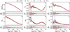 |
Fig. 5. Mean scaling relations between halo number density and selected non-local halo properties across different f(R) cosmologies at redshift z = 0.5. The properties plotted are Vmax, ℰh, ℳ5, Δ5, 𝒟5, and 𝒯A. The lower panels show the ratio of each property in f(R) with respect to ΛCDM. The error bars represent the uncertainty in the mean for each mass bin. |
For the neighbour statistics, 𝒟5, we observe that the MG models generally follow the overall trend of the ΛCDM model. In the lower panel of Fig. 5e, the ratio of neighbour statistics of MG to ΛCDM, 𝒟5MG/𝒟5CDM, fluctuates around 1%, indicating only minor deviations from the reference model. The F6 family of models remains virtually indistinguishable from ΛCDM, whereas the neighbour statistics in F5 models exhibit some significant variations. In this case, 𝒟5 shows fluctuations at low number densities ( ), with deviations reaching up to approximately 5% relative to the ΛCDM. As the number density increases, the ratio stabilises, remaining within 1%, which suggests that the F5 models align closely with standard gravity at higher densities. A slight turnaround is observed around
  , where the ratio dips just below 1% before recovering. Beyond this point, the neighbour statistics consistently remain below 3%, further indicating their close alignment with ΛCDM at higher densities. Lastly, and equally important, we analyse the triaxiality of MG halos. In the Fig. 5f, we observe that the results from MG models align with the overall trend of halo triaxiality of standard gravity. Focusing on the ratio of triaxiality (see the lower panel), at low number densities (
 ), the measurements are scattered enough to not show any conclusive departures from ΛCDM. However, beyond this threshold, a small deviation becomes apparent in all MG models, remaining constant up to
  . This deviation is around 1% for the F51 model and below 1% for the F52 and the remaining F6 models. Notably, triaxiality is the only property where we observe an effect of the power index of MG.
Table 1 presents the percent differences of the scaling relations for three non-local halo properties in f(R) models relative to the ΛCDM model, i.e., 100(ΘMG/ΘΛCDM − 1)[%], as a function of the mean number density. The table includes the properties 𝒟5 (first row, dark grey), ℳ5 (second row, medium grey), and Δ5 (third row, white), which are the ones that exhibit the largest deviations from standard gravity across different number density. Notably, these deviations are most pronounced for low-mass halos (higher number densities). We see that the quantity showing the largest deviation from ΛCDM is the local overdensity across most of the number density range, as already shown in Fig. 5. Specifically, for model F51, Δ5 is approximately 4% lower than the value expected in ΛCDM at ![Mathematical equation: $ \bar{n} \approx 6.43 \, [h^{-1} \, \mathrm{Mpc}]^{-3} $](/articles/aa/full_html/2025/08/aa55018-25/aa55018-25-eq20.gif) , while considering the power index n = 2, this difference decreases to about 3.3%. For the F6 models, the local overdensities remain below 1% over a wide range of number densities.
, while considering the power index n = 2, this difference decreases to about 3.3%. For the F6 models, the local overdensities remain below 1% over a wide range of number densities.
Percent differences in nonlocal halo property scaling relations for f(R) models relative to ΛCDM at z = 0.5
Figure 6 shows the relative mean scaling relations in the cosmic web for f(R) cosmologies as a function of number density at redshift z = 0.5. Each row displays the behaviour of a property –Vmax, ℰh, ℳ5, Δ5, 𝒟5, and 𝒯A– across different cosmic web environments: knots, filaments, sheets, and voids, as labelled in the columns6. As in previous figures, the error bars represent the uncertainty in the mean for each number density bin, and the grey region indicates a 5% error reference. We observe that sheets and voids are the most sensitive cosmic environments, showing notable differences when modifications to gravity are considered. The other environments, knots and filaments, are relatively insensitive to variations in the gravity model, with any discrepancies from ΛCDM remaining below 5% for all the f(R) models considered. In the case of sheets, however, the differences are above 5% compared to ΛCDM, especially for properties like the local Mach number, local overdensity, neighbour statistics, and tidal anisotropy of halos. This can be attributed to the fact that sheets are regions of intermediate density, positioned between dense clusters and less dense voids. Consequently, the impact of modified gravity on the local overdensity causes halos in sheets to evolve differently compared to those in more extreme environments. In sheets, the halo abundance is neither as high as in clusters nor as sparse as in voids, indicating a balanced density of halos.
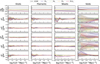 |
Fig. 6. Relative mean scaling relations in the cosmic web. The lines represent different halo properties in f(R) cosmologies as a function of number density at redshift z = 0.5. The rows show the ratio ΘMG/ΘΛCDM for the properties Vmax, ℰh, ℳ5, Δ5, 𝒟5, and 𝒯A. Each column corresponds to a different element of the cosmic web classification, i.e., knots, filaments, sheets, and voids. The error bars represent the uncertainty in the mean for each number density bin. |
An interesting feature observed in the properties of halos within sheets, such as tidal anisotropy, local overdensity, and Mach number, is that this environment appears to maximise the impact of the power index of MG as shown in Fig. 6. For the model F52, these properties closely align with ΛCDM, with deviations well below 5%. However, for F51, significant differences emerge with respect to ΛCDM: 5% in ℳ5 at  ; 12% in Δ5 at
  ; and 15% in 𝒯A at
  . A similar trend is observed when comparing F61 with F62, where differences with respect to ΛCDM are 7% in ℳ5; 10% in Δ5, and 15% in 𝒯A, for the same number density values as those for F5 models. These findings suggest a potential connection between the power index of f(R) and the evolution of large-scale structures in sheets. However, a more detailed investigation of this trend is beyond the scope of this paper and may be the subject of future work.
4.2. Secondary bias
The signal of the clustering of DM halos has been shown to depend on various secondary halo properties, rather than only halo mass. The secondary bias refers to the clustering of a population of matter tracers selected based on a secondary property, as a function of a primary property–in this case, the halo number density. The secondary bias is calculated by dividing the sample into quartiles of the secondary property and measuring the mean effective halo bias in bins of halo number density (for details on the procedure, see e.g. Montero-Dorta et al. 2020; Montero-Dorta & Rodriguez 2024; Balaguera-Antolínez et al. 2024). In this work, we focus on six representative secondary properties: Vmax, ℰh, M5, Δ5, D5, and 𝒯a.
Figures 7 and 8 show the measurements of mean effective bias in the first (lower) and fourth (upper) quartiles of all these properties for f(R) models with power index n = 1 and n = 2, respectively, with the ΛCDM results as reference in both cases (black data points). All the properties shown in these figures exhibit signatures of secondary bias, with significance that vary with number density, but overall remains stable across the different f(R) models. In fact, we see that the f(R) models considered, closely mimic the secondary bias of ΛCDM. This is evidenced by the agreement in bias signature between the two quartiles, indicating that these type of halo properties do not exhibit significant secondary bias; for example, Vmax and ℰh. On the other hand, properties such as ℳ5, Δ5, 𝒟5, and 𝒯A display, as was expected, clear secondary bias signatures (see, for example Balaguera-Antolínez et al. 2024; Balaguera-Antolínez & Montero-Dorta 2024, for a comparison).
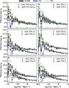 |
Fig. 7. Secondary halo bias: mean halo effective bias |

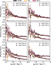 |
Fig. 8. Same as Fig. 7 but for the remaining MG models, F52 (orange) and F6.52 (dark purple) alongside results from the ΛCDM reference (black), all of them at the same redshift, z = 0.5. |
To quantify the extent of deviation in the secondary bias of f(R) models with respect to ΛCDM, we computed the significance of the signal, defined as
 (4)
(4)
where ⟨bh|θp⟩i(s) represents the mean sample bias measured in bins of the primary property θp for the i-th quartile of the secondary property θs. The standard error of the mean bias in the i-th quartile of the secondary property is denoted by σs, i. In our analysis, i = 4 and j = 1 correspond to the fourth (upper) and first (lower) quartiles, respectively. Therefore, the significance is  , with p representing
  and s being one of the secondary properties: Vmax, ℰh, ℳ5, Δ5, 𝒟5, and 𝒯A. One statistical indicator of a secondary halo bias signature is a significance value considerably higher than 1. This is important because some secondary qualities may have a large signal within a specific mass range (number density), but this signal might not be statistically significant. Figure 9 shows the statistical significance of the secondary halo bias as a function of halo number density for the different f(R) models (coloured lines) and ΛCDM (black lines).
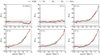 |
Fig. 9. Significance of the secondary halo bias as a function of number density, computed using Eq. (4) for different f(R) models and for the secondary properties: Vmax, ℰh, ℳ5, Δ5, 𝒟5, and 𝒯A. The dark-shaded stripe denotes a strip of |


Properties such as ℳ5, Δ5, 𝒟5, and 𝒯A clearly show a secondary bias, consistent with the results from Balaguera-Antolínez et al. (2024) for ΛCDM using the UNIT simulation. Figure 9 extends these findings to a variety of f(R) gravity models, where the strength of the secondary bias signal remains similar across all the models considered. The figure illustrates how the statistical significance changes with halo number density for the selected properties, with an uncertainty range of  included. Notably, as number density increases, the significance of the bias increases monotonically. Figure 9 shows that distinguishing the f(R) models from ΛCDM require measurements with (sub)percent precision in multiple number density bins, especially those for very massive and rare halos. Fortunately, near-future surveys expect to achieve this.
Our analysis reveals that, across all f(R) models studied, Vmax and ℰh do not exhibit secondary bias, as expected. The remaining properties, instead, display a similar statistical significance of secondary bias. At a reference number density of ∼10−7 – consistent with the expected comoving number densities of surveys such as DESI and Euclid (see e.g. Euclid Collaboration: Mellier 2025; Zhou et al. 2023) – we do observe notable deviations. Specifically, the significance levels are 18 units for ℳ5, 28 for Δ5, 20 for 𝒟5, and 22 for 𝒯A, consistently across all f(R) models. These results hold irrespective of the power index or the fR0 parameter (see Fig. 9).
To quantify the bias, we employed the methodology described by Paranjape et al. (2018), which was later implemented by Contreras et al. (2021a) and Balaguera-Antolínez et al. (2024). This approach uses an object-by-object estimator to calculate halo bias and assess secondary bias signatures in DM halos identified with ROCKSTAR. Our results extend the findings reported in Balaguera-Antolínez et al. (2024) on secondary halo bias to the context of f(R) cosmologies for the first time, while also validating the method in the ΛCDM scenario.
5. Conclusions
In this work, we present the measurements of primary and secondary bias for DM halos, extracted from the high-resolution simulations of MG cosmologies introduced by García-Farieta et al. (2024). The MG models correspond to the Hu-Sawicki parametrisation of the f(R) function. We consider two sets of models, each defined by specific combinations of the fR0 and n parameters, chosen to represent models that remain consistent with current observational constraints. Specifically, we investigate four MG models in addition to the reference ΛCDM model, (|fR0|, n)∈{(10−5, 1), (10−6, 1), (10−5, 2), (10−6.5, 2)}, which are denoted as {F51, F61, F52, F6.52} throughout this work.
We have explored the signal of bias using a number of halo properties derived from the halo finder. Among these, intrinsic properties are the maximum circular velocity and halo ellipticity. As a primary property, we have used the mean number density (interpolated from each f(R) catalogue) instead of halo mass, as the latter depends also on the MG models used. We have also analysed the impact on environmental properties such as the Mach number and the neighbour statistics, introduced by Balaguera-Antolínez et al. (2024). Our main conclusions can be summarised as follows:
-
The relative difference in the effective bias among the f(R) models when compared to ΛCDM, encodes information of the power index impact on the bias. For a fixed power index n = 1, the halo bias decreases as |fR0| increases, with maximum deviations of about 5%. This occurs because halos with a fixed number density become more abundant, leading to a bias reduction. This result is consistent with previous studies such as Schmidt et al. (2009), where the largest deviations from GR appear in low-mass halos. However, when the power index is fixed at n = 2, the suppression of the halo bias with respect to ΛCDM is no longer evident. Instead, the bias remains consistent across models with different |fR0|, such as F52 and F6.52, except for rare halos with low number densities. The impact of n manifests better in the F5 models, where increasing the power index reduces the suppression of the bias across a wide range of number densities.
-
The scaling relations for the full f(R) catalogues with the properties, Vmax, ℰh, ℳ5, Δ5, 𝒟5 and 𝒯A are presented in Fig. 5. Our analysis reveals that Vmax exhibits a nearly universal relationship with halo number density across all models, showing negligible deviations (< 1%) from ΛCDM. In contrast, halo ellipticity displays significant deviations (> 1%) only in the F5 models (for both power indices) within the low-mass range [1.20 × 10¹², 1.62 × 10¹³] h−1M⊙, while no notable differences arise at lower number densities (
 ). For the Mach number, departures from ΛCDM emerge at
  , with a monotonic increase in ℳ5 ratios beginning at
  , whereas the F6 models remain consistent across all densities. Similarly, the local overdensity shows no significant deviations in most models, except for the F5 family, where Δ5MG/Δ5ΛCDM decreases monotonically with increasing number density, unaffected by the power index.
 -
The halo properties studied through scaling relations were analysed across different environments of the cosmic web to quantify their environmental impact. The results show that sheets and voids are the most responsive environments to f(R), exhibiting deviations across multiple halo properties. In these environments, the tidal anisotropy, local overdensity, and Mach number appear to be sensitive to the power index of f(R), with differences exceeding 5% compared to ΛCDM, reaching up to 12% in Δ5 and 15% in 𝒯A for the F51 model. On the contrary, knots and filaments remain largely unaffected, with any discrepancy below 5%. We found that, while F52 closely aligns with ΛCDM (deviations < 5%), F51 and F61 exhibit stronger departures (e.g. 7–15% in ℳ5, Δ5, and 𝒯A), which hints at the impact of the power index on cosmic tracers that inhabit underdense regions. These findings suggest that traces of f(R) gravity are environment-dependent, with sheets and voids potentially serving as probes for deviations from GR.
-
The measurements of the secondary bias across halo properties (including Vmax, Eh, ℳ5, Δ5, 𝒟5, and 𝒯A), show a consistent behaviour that persists across all f(R) models. We found that the f(R) models closely reproduce the secondary bias of ΛCDM with high fidelity in all cases. We report that while properties such as Vmax and halo ℰh have a negligible secondary bias, as expected, ℳ5, Δ5, 𝒟5, and 𝒯A exhibit statistically significant trends, albeit remaining fully compatible with ΛCDM.
-
We quantified the extent of the deviation in the secondary bias of f(R) halos relative to ΛCDM by computing the significance of the signal, accounting for the intrinsic scatter in the measurements. For halo properties such as ℳ5, Δ5, 𝒟5, and 𝒯A, we find a statistical significance of the secondary bias consistent with the ΛCDM results reported by Balaguera-Antolínez et al. (2024). When extending this analysis to f(R) halos, the signal strength remains remarkably similar across all investigated parameter combinations, regardless of variations in both fR0 and the power index. In general, we do not find any statistically significant deviation from ΛCDM in the secondary halo bias for the different f(R) models explored in this work.
We anticipate several extensions of the analysis presented in this work. In particular, the set of simulations we have employed can be combined with various filament and void identification schemes to explore in more detail the sensitivity of the relationship between large-scale bias and the cosmic web to variations in the underlying cosmology.
The secondary dependencies directly related to the different accretion histories of halos are specifically called halo assembly bias.
The assignment of individual halo bias has been performed using the CosmiCCcodes library at https://github.com/balaguera/CosmicCodes.
We have used a maximum wavenumber of kmax = 0.08 h Mpc−1, up to which the ratio Ph(k)/Pdm(k) is compatible with a constant value at the current redshift.
Mvir is defined using the standard spherical overdensity criterion, with the commonly used value of Δvir for ΛCDM, obtained after applying the ROCKSTAR halo finder to the f(R) simulation snapshots (see e.g. Lombriser et al. 2014; Lee & Baldi 2022; Lee et al. 2023).
As in Balaguera-Antolínez et al. (2024), this classification is based on the eigenvalues of the tidal field setting a null threshold.
Acknowledgments
J.E. García-Farieta research was financially supported by the project “Plan Complementario de I+D+i en el área de Astrofísica” funded by the European Union within the framework of the Recovery, Transformation and Resilience Plan - NextGenerationEU and by the Regional Government of Andalucia (Reference AST22_00001). ABA acknowledges the Spanish Ministry of Economy and Competitiveness (MINECO) under the Severo Ochoa programme SEV-2015- 0548 grants. A.D. Montero-Dorta thanks Fondecyt for financial support through the Fondecyt Regular 2021 grant 1210612.
References
- Angulo, R. E., Baugh, C. M., & Lacey, C. G. 2008, MNRAS, 387, 921 [NASA ADS] [CrossRef] [Google Scholar]
- Arnalte-Mur, P., Hellwing, W. A., & Norberg, P. 2017, MNRAS, 467, 1569 [NASA ADS] [Google Scholar]
- Arnold, C., Puchwein, E., & Springel, V. 2014, MNRAS, 440, 833 [Google Scholar]
- Arnold, C., Springel, V., & Puchwein, E. 2016, MNRAS, 462, 1530 [Google Scholar]
- Artis, E., Ghirardini, V., Bulbul, E., et al. 2024, A&A, 691, A301 [NASA ADS] [CrossRef] [EDP Sciences] [Google Scholar]
- Aviles, A. 2025, Phys. Rev. D, 111, L021301 [Google Scholar]
- Balaguera-Antolínez, A. 2014, A&A, 563, A141 [NASA ADS] [CrossRef] [EDP Sciences] [Google Scholar]
- Balaguera-Antolínez, A., & Montero-Dorta, A. D. 2024, A&A, 692, A32 [NASA ADS] [CrossRef] [EDP Sciences] [Google Scholar]
- Balaguera-Antolínez, A., Montero-Dorta, A. D., & Favole, G. 2024, A&A, 685, A61 [NASA ADS] [CrossRef] [EDP Sciences] [Google Scholar]
- Bamba, K., Nojiri, S., & Odintsov, S. D. 2008, JCAP, 2008, 045 [Google Scholar]
- Bardeen, J. M., Bond, J. R., Kaiser, N., & Szalay, A. S. 1986, ApJ, 304, 15 [Google Scholar]
- Behroozi, P. S., Wechsler, R. H., & Wu, H.-Y. 2013, ApJ, 762, 109 [NASA ADS] [CrossRef] [Google Scholar]
- Berti, E., Barausse, E., Cardoso, V., et al. 2015, CQG, 32, 243001 [NASA ADS] [CrossRef] [Google Scholar]
- Casas, S., Cardone, V.F., Sapone, D., et al. 2023, arXiv e-prints [arXiv:2306.11053] [Google Scholar]
- Chudaykin, A., & Kunz, M. 2024, Phys. Rev. D, 110, 123524 [Google Scholar]
- Chudaykin, A., Kunz, M., & Carron, J. 2025, arXiv e-prints [arXiv:2503.09893] [Google Scholar]
- Clifton, T., Ferreira, P. G., Padilla, A., & Skordis, C. 2012, Phys. Rep., 513, 1 [NASA ADS] [CrossRef] [Google Scholar]
- Contarini, S., Marulli, F., Moscardini, L., et al. 2021, MNRAS, 504, 5021 [NASA ADS] [CrossRef] [Google Scholar]
- Contreras, S., Zehavi, I., Padilla, N., et al. 2019, MNRAS, 484, 1133 [NASA ADS] [CrossRef] [Google Scholar]
- Contreras, S., Angulo, R. E., & Zennaro, M. 2021a, MNRAS, 504, 5205 [CrossRef] [Google Scholar]
- Contreras, S., Chaves-Montero, J., Zennaro, M., & Angulo, R. E. 2021b, MNRAS, 507, 3412 [NASA ADS] [CrossRef] [Google Scholar]
- Corasaniti, P. S., Giocoli, C., & Baldi, M. 2020, Phys. Rev. D, 102, 043501 [Google Scholar]
- Crocce, M., Pueblas, S., & Scoccimarro, R. 2006, MNRAS, 373, 369 [NASA ADS] [CrossRef] [Google Scholar]
- Dainotti, M. G., De Simone, B., Garg, A., et al. 2025, J. High Energy Astrophys., 48, 100405 [Google Scholar]
- Dalal, N., White, M., Bond, J. R., & Shirokov, A. 2008, ApJ, 687, 12 [NASA ADS] [CrossRef] [Google Scholar]
- de Haro, J., Nojiri, S., Odintsov, S. D., Oikonomou, V. K., & Pan, S. 2023, Phys. Rep., 1034, 1 [Google Scholar]
- DESI Collaboration (Lodha, K., et al.) 2025, arXiv e-prints [arXiv:2503.14743] [Google Scholar]
- Euclid Collaboration (Mellier, Y., et al.) 2025, A&A, 697, A1 [Google Scholar]
- Faltenbacher, A., & White, S. D. M. 2010, ApJ, 708, 469 [NASA ADS] [CrossRef] [Google Scholar]
- Fiorini, B., Koyama, K., & Izard, A. 2022, JCAP, 2022, 028 [CrossRef] [Google Scholar]
- Frusciante, N., Pace, F., Cardone, V. F., et al. 2024, A&A, 690, A133 [NASA ADS] [CrossRef] [EDP Sciences] [Google Scholar]
- Gao, L., & White, S. D. M. 2007, MNRAS, 377, L5 [NASA ADS] [CrossRef] [Google Scholar]
- Gao, L., Springel, V., & White, S. D. M. 2005, MNRAS, 363, L66 [NASA ADS] [CrossRef] [Google Scholar]
- García-Farieta, J. E., Marulli, F., Veropalumbo, A., et al. 2019, MNRAS, 488, 1987 [Google Scholar]
- García-Farieta, J. E., Marulli, F., Moscardini, L., Veropalumbo, A., & Casas-Miranda, R. A. 2020, MNRAS, 494, 1658 [CrossRef] [Google Scholar]
- García-Farieta, J. E., Hellwing, W. A., Gupta, S., & Bilicki, M. 2021, Phys. Rev. D, 103, 103524 [CrossRef] [Google Scholar]
- García-Farieta, J. E., Balaguera-Antolínez, A., & Kitaura, F.-S. 2024, A&A, 690, A27 [NASA ADS] [CrossRef] [EDP Sciences] [Google Scholar]
- Gil-Marín, H., Schmidt, F., Hu, W., Jimenez, R., & Verde, L. 2011, JCAP, 2011, 019 [CrossRef] [Google Scholar]
- Giocoli, C., Baldi, M., & Moscardini, L. 2018, MNRAS, 481, 2813 [Google Scholar]
- Gupta, S., Hellwing, W. A., Bilicki, M., & García-Farieta, J. E. 2022, Phys. Rev. D, 105, 043538 [NASA ADS] [CrossRef] [Google Scholar]
- Hagstotz, S., Costanzi, M., Baldi, M., & Weller, J. 2019, MNRAS, 486, 3927 [Google Scholar]
- Hahn, O., Porciani, C., Carollo, C. M., & Dekel, A. 2007, MNRAS, 375, 489 [NASA ADS] [CrossRef] [Google Scholar]
- Han, J., Li, Y., Jing, Y., et al. 2019, MNRAS, 482, 1900 [NASA ADS] [CrossRef] [Google Scholar]
- Hernández-Aguayo, C., Hou, J., Li, B., Baugh, C. M., & Sánchez, A. G. 2019, MNRAS, 485, 2194 [CrossRef] [Google Scholar]
- Hu, W., & Sawicki, I. 2007, Phys. Rev. D, 76, 064004 [CrossRef] [Google Scholar]
- Ishak, M., Pan, J., Calderon, R., et al. 2024, arXiv e-prints [arXiv:2411.12026] [Google Scholar]
- Jennings, E., Baugh, C. M., Li, B., Zhao, G.-B., & Koyama, K. 2012, MNRAS, 425, 2128 [NASA ADS] [CrossRef] [Google Scholar]
- Johnson, J. W., Maller, A. H., Berlind, A. A., Sinha, M., & Holley-Bockelmann, J. K. 2019, MNRAS, 486, 1156 [CrossRef] [Google Scholar]
- Kaiser, N. 1984, ApJ, 284, L9 [NASA ADS] [CrossRef] [Google Scholar]
- Khoury, J., & Weltman, A. 2004, Phys. Rev. D, 69, 044026 [CrossRef] [Google Scholar]
- Koyama, K. 2016, Rep. Prog. Phys, 79, 046902 [Google Scholar]
- Landim, R. G., Desmond, H., Koyama, K., & Penny, S. 2024, MNRAS, 534, 349 [Google Scholar]
- Laureijs, R., Amiaux, J., Arduini, S., et al. 2011, arXiv e-prints [arXiv:1110.3193] [Google Scholar]
- Lazeyras, T., Musso, M., & Schmidt, F. 2017, JCAP, 2017, 059 [Google Scholar]
- Lee, J., & Baldi, M. 2022, ApJ, 938, 137 [NASA ADS] [CrossRef] [Google Scholar]
- Lee, J., Ryu, S., & Baldi, M. 2023, ApJ, 945, 15 [NASA ADS] [CrossRef] [Google Scholar]
- Li, Y., Mo, H. J., & Gao, L. 2008, MNRAS, 389, 1419 [NASA ADS] [CrossRef] [Google Scholar]
- Liu, X., Li, B., Zhao, G.-B., et al. 2016, Phys. Rev. Lett., 117, 051101 [NASA ADS] [CrossRef] [Google Scholar]
- Liu, W., Wu, L., Villaescusa-Navarro, F., et al. 2025, JCAP, 2025, 088 [Google Scholar]
- Lombriser, L., Koyama, K., & Li, B. 2014, JCAP, 2014, 021 [Google Scholar]
- Maggiore, L., Contarini, S., Giocoli, C., & Moscardini, L. 2025, A&A, in press, https://doi.org/10.1051/0004-6361/202554968 [Google Scholar]
- Mao, Y.-Y., Zentner, A. R., & Wechsler, R. H. 2018, MNRAS, 474, 5143 [NASA ADS] [CrossRef] [Google Scholar]
- Mo, H. J., & White, S. D. M. 1996, MNRAS, 282, 347 [Google Scholar]
- Montero-Dorta, A. D., & Rodriguez, F. 2024, MNRAS, 531, 290 [NASA ADS] [CrossRef] [Google Scholar]
- Montero-Dorta, A. D., Artale, M. C., Abramo, L. R., et al. 2020, MNRAS, 496, 1182 [NASA ADS] [CrossRef] [Google Scholar]
- Montero-Dorta, A. D., Chaves-Montero, J., Artale, M. C., & Favole, G. 2021, MNRAS, 508, 940 [NASA ADS] [CrossRef] [Google Scholar]
- Montero-Dorta, A. D., Contreras, S., Artale, M. Celeste, Rodriguez, F., & Favole, G. 2025, A&A, 695, A159 [NASA ADS] [CrossRef] [EDP Sciences] [Google Scholar]
- Nojiri, S., Odintsov, S. D., & Oikonomou, V. K. 2017, Phys. Rep., 692, 1 [NASA ADS] [CrossRef] [Google Scholar]
- Odintsov, S. D., Sáez-Chillón Gómez, D., & Sharov, G. S. 2024, arXiv e-prints [arXiv:2412.09409] [Google Scholar]
- Paranjape, A., & Alam, S. 2020, MNRAS, 495, 3233 [NASA ADS] [CrossRef] [Google Scholar]
- Paranjape, A., Hahn, O., & Sheth, R. K. 2018, MNRAS, 476, 3631 [NASA ADS] [CrossRef] [Google Scholar]
- Peel, A., Pettorino, V., Giocoli, C., Starck, J.-L., & Baldi, M. 2018, A&A, 619, A38 [NASA ADS] [CrossRef] [EDP Sciences] [Google Scholar]
- Peel, A., Lalande, F., Starck, J.-L., et al. 2019, Phys. Rev. D, 100, 023508 [Google Scholar]
- Perico, E. L. D., & Tamayo, D. A. 2017, JCAP, 2017, 026 [CrossRef] [Google Scholar]
- Planck Collaboration VI. 2020, A&A, 641, A6 [NASA ADS] [CrossRef] [EDP Sciences] [Google Scholar]
- Plaza, F., & Kraiselburd, L. 2025, arXiv e-prints [arXiv:2503.16132] [Google Scholar]
- Pollack, J. E., Smith, R. E., & Porciani, C. 2012, MNRAS, 420, 3469 [NASA ADS] [CrossRef] [Google Scholar]
- Pollack, J. E., Smith, R. E., & Porciani, C. 2014, MNRAS, 440, 555 [CrossRef] [Google Scholar]
- Ramakrishnan, S., Paranjape, A., Hahn, O., & Sheth, R. K. 2019, MNRAS, 489, 2977 [NASA ADS] [CrossRef] [Google Scholar]
- Salcedo, A. N., Maller, A. H., Berlind, A. A., et al. 2018, MNRAS, 475, 4411 [NASA ADS] [CrossRef] [Google Scholar]
- Sato-Polito, G., Montero-Dorta, A. D., Abramo, L. R., Prada, F., & Klypin, A. 2019, MNRAS, 487, 1570 [NASA ADS] [CrossRef] [Google Scholar]
- Schmidt, F., Lima, M., Oyaizu, H., & Hu, W. 2009, Phys. Rev. D, 79, 083518 [NASA ADS] [CrossRef] [Google Scholar]
- Scoccimarro, R. 1998, MNRAS, 299, 1097 [NASA ADS] [CrossRef] [Google Scholar]
- Sheth, R. K., & Tormen, G. 1999, MNRAS, 308, 119 [Google Scholar]
- Sheth, R. K., & Tormen, G. 2004, MNRAS, 350, 1385 [NASA ADS] [CrossRef] [Google Scholar]
- Sheth, R. K., Mo, H. J., & Tormen, G. 2001, MNRAS, 323, 1 [NASA ADS] [CrossRef] [Google Scholar]
- Smith, R. E., Scoccimarro, R., & Sheth, R. K. 2007, Phys. Rev. D, 75, 063512 [NASA ADS] [CrossRef] [Google Scholar]
- Sotiriou, T. P., & Faraoni, V. 2010, Rev. Mod. Phys., 82, 451 [NASA ADS] [CrossRef] [Google Scholar]
- Tinker, J. L., Robertson, B. E., Kravtsov, A. V., et al. 2010, ApJ, 724, 878 [NASA ADS] [CrossRef] [Google Scholar]
- Tucci, B., Montero-Dorta, A. D., Abramo, L. R., Sato-Polito, G., & Artale, M. C. 2021, MNRAS, 500, 2777 [Google Scholar]
- van de Weygaert, R., & Schaap, W. 2009, in Data Analysis in Cosmology, eds. V. J. Martínez, E. Saar, E. Martínez-González, & M. J. Pons-Bordería (Berlin Heidelberg: Springer), 665, 291 [NASA ADS] [CrossRef] [Google Scholar]
- Vogt, S. M. L., Bocquet, S., Davies, C. T., et al. 2025, Phys. Rev. D, 111, 043519 [NASA ADS] [CrossRef] [Google Scholar]
- Voivodic, R., Lima, M., Llinares, C., & Mota, D. F. 2017, Phys. Rev. D, 95, 024018 [CrossRef] [Google Scholar]
- Wechsler, R. H., Zentner, A. R., Bullock, J. S., Kravtsov, A. V., & Allgood, B. 2006, ApJ, 652, 71 [NASA ADS] [CrossRef] [Google Scholar]
- Wright, B. S., Koyama, K., Winther, H. A., & Zhao, G.-B. 2019, JCAP, 2019, 040 [CrossRef] [Google Scholar]
- Zhou, R., Dey, B., Newman, J. A., et al. 2023, AJ, 165, 58 [NASA ADS] [CrossRef] [Google Scholar]
- Zivick, P., Sutter, P. M., Wandelt, B. D., Li, B., & Lam, T. Y. 2015, MNRAS, 451, 4215 [NASA ADS] [CrossRef] [Google Scholar]
All Tables
Percent differences in nonlocal halo property scaling relations for f(R) models relative to ΛCDM at z = 0.5
All Figures
|
Fig. 1. Slices of the ∼12 h−1Mpc thickness in the MG simulations (at z = 0.5) showing the individual bias field. The zoom-in region represents a 100 × 100 h−2Mpc−2 slice. |
| In the text | |
|
Fig. 2. Cumulative halo mass function for the different MG models taken at redshift z = 0.5. The bottom panel shows the relative deviation with respect to the ΛCDM model with lines connecting the data points to guide the eye. |
| In the text | |
|
Fig. 3. Halo effective bias, bhm, computed at z = 0.5 as a function of the number density. The points denote the mean bias in different mass bins, with errorbars denoting the standard error of the mean. The contours indicate a region of an equal number of tracers Nh. |
| In the text | |
|
Fig. 4. Ratios of the effective halo bias in the f(R) simulations at z = 0.5, measured in bins of the halo viral mass. Symbols denote the mean halo-mass bias ⟨bhm|logMvir⟩. |
| In the text | |
|
Fig. 5. Mean scaling relations between halo number density and selected non-local halo properties across different f(R) cosmologies at redshift z = 0.5. The properties plotted are Vmax, ℰh, ℳ5, Δ5, 𝒟5, and 𝒯A. The lower panels show the ratio of each property in f(R) with respect to ΛCDM. The error bars represent the uncertainty in the mean for each mass bin. |
| In the text | |
|
Fig. 6. Relative mean scaling relations in the cosmic web. The lines represent different halo properties in f(R) cosmologies as a function of number density at redshift z = 0.5. The rows show the ratio ΘMG/ΘΛCDM for the properties Vmax, ℰh, ℳ5, Δ5, 𝒟5, and 𝒯A. Each column corresponds to a different element of the cosmic web classification, i.e., knots, filaments, sheets, and voids. The error bars represent the uncertainty in the mean for each number density bin. |
| In the text | |
|
Fig. 7. Secondary halo bias: mean halo effective bias |
| In the text | |
|
Fig. 8. Same as Fig. 7 but for the remaining MG models, F52 (orange) and F6.52 (dark purple) alongside results from the ΛCDM reference (black), all of them at the same redshift, z = 0.5. |
| In the text | |
|
Fig. 9. Significance of the secondary halo bias as a function of number density, computed using Eq. (4) for different f(R) models and for the secondary properties: Vmax, ℰh, ℳ5, Δ5, 𝒟5, and 𝒯A. The dark-shaded stripe denotes a strip of |
| In the text | |
Current usage metrics show cumulative count of Article Views (full-text article views including HTML views, PDF and ePub downloads, according to the available data) and Abstracts Views on Vision4Press platform.
Data correspond to usage on the plateform after 2015. The current usage metrics is available 48-96 hours after online publication and is updated daily on week days.
Initial download of the metrics may take a while.