| Issue |
A&A
Volume 700, August 2025
|
|
|---|---|---|
| Article Number | L17 | |
| Number of page(s) | 5 | |
| Section | Letters to the Editor | |
| DOI | https://doi.org/10.1051/0004-6361/202555311 | |
| Published online | 15 August 2025 | |
Letter to the Editor
SN 2022jli modeled with a 56Ni double layer and a magnetar
1
Laboratorio de Investigación Científica en Astronomía, UNRN, Sede Andina, Mitre 630 (8400), Bariloche, Argentina
2
Consejo Nacional de Investigaciones Científicas y Técnicas (CONICET), Godoy Cruz 2290, Buenos Aires, Argentina
3
Instituto de Astrofísica de La Plata (IALP), CCT-CONICET-UNLP, Paseo del Bosque s/n, B1900FWA La Plata, Argentina
4
Facultad de Ciencias Astronómicas y Geofísicas, UNLP, Paseo del Bosque s/n, 1900 La Plata, Buenos Aires, Argentina
5
Kavli IPMU (WPI), UTIAS, The University of Tokyo, Kashiwa, Chiba 277-8583, Japan
6
Institut d’Estudis Espacials de Catalunya (IEEC), Edifici RDIT, Campus UPC, 08860 Castelldefels, (Barcelona), Spain
7
Institute of Space Sciences (ICE, CSIC), Campus UAB, Carrer de Can Magrans, s/n, E-08193 Barcelona, Spain
⋆ Corresponding author: This email address is being protected from spambots. You need JavaScript enabled to view it.
Received:
27
April
2025
Accepted:
25
July
2025
Abstract
Context. We study the bolometric evolution of the exceptional Type Ic supernova SN 2022jli, aiming to understand the underlying mechanisms responsible for its distinctive double-peaked light curve morphology, extended timescales, and the rapid, steep decline in luminosity observed at around 270 days after the SN discovery.
Aims. We present a quantitative assessment of two leading models through the use of hydrodynamic radiative simulations: two shells enriched with nickel and a combination of nickel and magnetar power.
Methods. We explored the parameter space of a model in which the supernova (SN) is powered by radioactive decay while assuming a bimodal nickel distribution. Though this setup can reproduce the early light curve properties, it faces problems explaining the prominent second peak. We therefore considered a hybrid scenario with a rapidly rotating magnetar as an additional energy source.
Results. We find that the observed light curve morphology can be well reproduced by a model combining a magnetar engine and a double-layer 56Ni distribution. The best-fitting case consists of a magnetar with a spin period of P ≃ 22 ms and a bipolar magnetic field strength of B ≃ 5 × 10¹⁴ G and a radioactive content with a total M(56Ni) of 0.15 M⊙ distributed across two distinct shells within a pre-SN structure of 11 M⊙. To reproduce the abrupt drop in luminosity at ∼270 d, the energy deposition from the magnetar must be rapidly and effectively switched off.
Key words: supernovae: general / supernovae: individual: SN 2022jli
© The Authors 2025
 Open Access article, published by EDP Sciences, under the terms of the Creative Commons Attribution License (https://creativecommons.org/licenses/by/4.0), which permits unrestricted use, distribution, and reproduction in any medium, provided the original work is properly cited.
This article is published in open access under the Subscribe to Open model. This email address is being protected from spambots. You need JavaScript enabled to view it. to support open access publication.
1. Introduction
Type Ic supernovae (SNe Ic) are thought to be core-collapse SNe resulting from the final explosion of massive stars that have been stripped of both their hydrogen and helium envelopes before the explosion. Their spectra are defined by the absence of hydrogen and helium lines (e.g. Filippenko 1997; Gal-Yam 2017; Modjaz et al. 2019). Although the mechanism of total helium removal remains an open question in stellar evolution (Ertl et al. 2020), SNe Ic progenitors are debated to be either very massive stars that lose their outer layers through strong stellar winds (Heger et al. 2003; Georgy et al. 2009) or stars in binary systems that were stripped via interaction with a companion (e.g., Podsiadlowski et al. 1992; Nomoto et al. 1995; Eldridge et al. 2008).
The observed diversity among SNe Ic has grown significantly in recent years, largely thanks to the advent of wide-field sky surveys. One remarkable example is SN 2022jli. The optical light curves of this SN displayed an unusual re-brightening approximately one month after discovery, as reported by Moore et al. (2023), Chen et al. (2024), Cartier et al. (2024). A conspicuous second peak comparable in luminosity to the first peak reached maximum light around ≳59 days post-discovery, making this an unprecedented light curve (LC). Cartier et al. (2024) determined the epoch of the first maximum brightness (tmax) of this LC to be MJD = 59709.6 ± 1.2 days based on a polynomial fit. This corresponds to roughly five days after its discovery on 2022 May 5 (Monard 2022). However, the explosion time remains poorly constrained, with the last non-detection occurring 87.5 days before the discovery (Chen et al. 2024).
The relatively nearby distance of SN 2022jli (∼23 Mpc; Moore et al. 2023) enabled high-cadence follow-up through extensive photometric and spectroscopic campaigns. One of the most remarkable features of SN 2022jli is the presence of periodic fluctuations in its light curves during the decline phase. These modulations, with a period of 12.4 days and an amplitude of ∼1% of the SN’s peak luminosity, persist for at least ∼200 days (Moore et al. 2023). Spectroscopically, helium lines are weak, while hydrogen lines become visible only after the second peak. Notably, the Hα feature begins to exhibit a periodic shift in its peak, following the LC undulations (Cartier et al. 2024). Chen et al. (2024) suggest a tentative association with a Fermi γ-ray source, although no corresponding emission was detected in the radio or X-ray bands. Cartier et al. (2024) further extended the optical and near-infrared monitoring of SN 2022jli up to 600 days after discovery, revealing a significant near-infrared (NIR) excess from hot dust emission around ∼238 days.
Assuming the explosion of SN 2022jli occurred shortly before its discovery, its bolometric LC has some resemblance to other stripped-envelope SNe, such as SN 2005bf (Folatelli et al. 2006), SN 2008D (Soderberg et al. 2008; Chevalier & Fransson 2008; Modjaz et al. 2009), PTF11mnb (Taddia et al. 2018), and SN 2019cad (Gutiérrez et al. 2021). These events were similarly discovered during a phase of early rise prior to the first peak of the LC and have been modeled successfully using a double distribution of 56Ni. In this context, the LC morphology of SN 2022jli provides a compelling case for testing both the double 56Ni parametric power models (Orellana & Bersten 2022) and the hybrid models combining radioactive decay and magnetar power source, which have also been proposed for PFT11mnb (Taddia et al. 2018) and SN2019cad (Gutiérrez et al. 2021).
While various competing scenarios have already been discussed in the literature (Moore et al. 2023; Chen et al. 2024; Cartier et al. 2024), detailed hydrodynamic calculations can achieve a more robust assessment. Moore et al. (2023) considered several interpretations, including a combination of early shock-cooling emission from interaction with a circumstellar material (CSM) and a subsequent radioactively powered main peak. Using the MOSFiT code by Nicholl et al. (2017), they found that explaining the duration of the early excess required a substantial CSM mass (> 3 M⊙), which is unusually high for a Type Ic SN. This would require an exotic mass-loss mechanism shortly before the explosion. Moreover, a dense CSM structure attached to the progenitor star would likely be inconsistent with the observed early bolometric LC rise. Their modeling also implied a rather large nickel mass, M(56Ni) = fNi Mej = 0.234 M⊙, which adds further complications. This scenario could be further explored, posing a combination between CSM and magnetar, but a detailed analysis of the CSM case is beyond the focus of this work.
Accretion-powered scenarios have also been discussed as possible explanations for the late-time luminosity evolution. While not ruled out, such models and mechanisms involving collision with a binary companion remain speculative and require further investigation. Particularly, the periodic LC undulations were attributed to binarity (Chen et al. 2024), a hypothesis that has since been revised by King & Lasota (2024), who proposed that SN 2022jli may mark the ultraluminous birth of a low-mass X-ray binary.
More recently, Cartier et al. (2024) explored a scenario in which the first peak is powered by radioactive decay, which they modeled using Arnett’s prescriptions, while a magnetar powers the second peak. Their semi-analytic one-zone model based on Kasen & Bildsten (2010) reproduces the observed LC but requires the magnetar to be artificially activated ∼37 days after the explosion: a significant caveat that lacks a clear physical justification. Furthermore, their dataset is temporally sparse compared to the more densely sampled observations presented by Chen et al. (2024). We use the latter observational data in this work, which include their construction of Lpseudo = LBVRI + LNIR and a suitable correction to obtain Lbol1.
To quantitatively test the leading scenarios and understand the LC morphology of SNe 2022jli, we adopted the radiation hydrodynamic modeling framework developed by Orellana & Bersten (2022) based on a one-dimensional local thermodynamic equilibrium code (Bersten et al. 2011). This method enables us to distinguish between competing models involving either a double-peaked nickel distribution or a hybrid of nickel decay and magnetar power. Our approach is compatible with a range of physical configurations, including explosions in binary systems (Chrimes et al. 2022; Wei et al. 2024, and references) or non-standard explosion mixing-out some radioactive material (e.g., Aloy & Obergaulinger 2021). In particular, the stratified nickel structure observed in SN 2005bf-like events has been attributed to jet-like outflows during core collapse, a scenario that may also apply to SN 2022jli. Here we focus on reproducing the general evolution of the bolometric LC from early epochs but we do not attempt to explain the periodic variability in SN 2022jli.
2. Modeling the light curve with two 56Ni shells
Orellana & Bersten (2022) aimed to explain some of the diversity seen in the LC morphologies of double-peaked SNe, highlighting that an initial bolometric rise before the two peaks, such as observed in SN 2022jli, can be explained by a bimodal distribution of radioactive nickel. Their study showed that when the LC maxima are separated from each other by a long interval, typically of the order of a month, a massive progenitor is required. This ensures sufficient spatial separation of the 56Ni components in the mass coordinate, allowing their distinct influence on the LC to manifest at different times. A nickel-poor zone between these two shells enables a marked dip between the peaks, as is the case for SN 2022jli. That reasoning motivates our choice of a pre-SN structure with a relatively large mass. Here we prefer a progenitor structure that we refer to as He11 and which corresponds to a zero age main sequence mass of 30 M⊙ evolved using the MESA code (Paxton et al. 2011). For our He11 model, the ejected mass is 9.55 M⊙, which is consistent with the mass ranges estimated by Moore et al. (2023), who inferred Mej ≈ 12 ± 6 M⊙ based on the long rise to the second maximum.
After setting the progenitor mass, the explosion energy, Eexp, must be sufficiently high to impulse the massive ejecta and reproduce the observed photospheric velocities. Spectroscopic measurements at ≈16 days post explosion suggest an average Fe II velocity of  km s−1 (Cartier et al. 2024). We experimented with several energy values and ultimately adopted Eexp = 3 × 1051 erg for our simulation. This choice adequately reproduces the maximum measured velocity, though we do not intend to reproduce the entire velocity evolution. In all the calculations, we adopted a constant gamma-ray opacity of κγ = 0.03 cm2/g.
Following the formalism of Orellana & Bersten (2022), we performed one-dimensional radiative transfer hydrodynamic calculations where we varied the fractional mass coordinates for the He11 structure with different configurations of the two 56Ni enriched shells. The inner shell is located between f0 ⋅ Mej and f1 ⋅ Mej in terms of mass coordinates, and the outer shell is located between f2 ⋅ Mej and f3 ⋅ Mej. The corresponding abundances of nickel are Xin and Xout, respectively.
The first LC peak occurs approximately five days after discovery (see Figure 1), with a bolometric peak luminosity of L ∼ 1042.5 erg s−1, which can be explained by radioactive heating from the external 56Ni shell extending up to f3 = 0.99. Thus, it nearly reaches the stellar surface. However, this outer extent is poorly constrained, as it is sensitive to the assumed explosion time. In our preferred model, the first maximum occurs around 13 days post explosion. However, given the scarcity of early data (during the first ascent) and the large uncertainty associated with the timing of the explosion, the exact shape of the early LC is not entirely clear, and the same applies to the parameters obtained from its modeling. Therefore, we caution against over-interpreting the shape of the first peak.
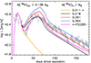 |
Fig. 1. Light curve comparison between the SN observations (gray markers; Chen et al. 2024 bolometric) and the bolometric output from our double-peaked 56Ni distribution model. The inner component of the distribution is varied, while a fixed outer component of the profile is set to provide a reasonable fit for the first maximum of the LC. The model including a magnetar component is shown in magenta. In all the cases, the external enriched 56Ni shell is fixed, and the progenitor is the He11, as detailed in the text. |
The subsequent LC decline over the following 20 days is consistent with the outer shell having an inner boundary at about f2 ≃ 0.85 and Xout ≃ 0.09. This outer component contains approximately 0.138 M⊙ of 56Ni. For a total M(56Ni) of 0.15 M⊙ (as estimated by Chen et al. 2024 and consistent with other SNe Ic), the inner shell contains 0.011 M⊙ of nickel. The resulting profile is inverted, with higher 56Ni abundance in the outer layers. However, this inversion is less extreme than in SN 2008D models found by Bersten et al. (2013) due to the different timescales involved. Inverted double nickel profiles can be expected in combination with jet-like outflows that might be responsible for the external placing of nickel (Piran et al. 2019; Bugli et al. 2021) or mixing instabilities (Hammer et al. 2010 and see also the arguments in Orellana & Bersten 2022).
To test whether the second LC maximum at ∼60 d could be powered solely by the inner 56Ni component, we allowed the total M(56Ni) to vary freely between 0.138 and 0.6 M⊙. For a compact object, namely a neutron star of Mco = 1.45 M⊙, the innermost boundary corresponds to f0 = 0.132. After exploring different configurations, we found that a second peak consistent in time with the data can be obtained for f1 = 0.2.
Figure 1 shows our results for the double 56Ni distribution models contrasted with the bolometric data of SN 2022jli. We note that these models are not fully satisfactory. If we adjust the model to match the second maximum, the late-time data (> 100 days) is significantly underestimated (black line of Fig. 1). Conversely, if the late decline is well reproduced, the second peak appears overluminous (red and blue lines of Fig. 1). Moreover, the LC minimum brightness around ∼30 d, between the two peaks, is difficult to reproduce under this scenario. If the nickel-alone scenario were to account for the late steep decline observed at ∼270 d in Chen et al. (2024) data, a strong change in the 56Ni energy leakage should be invoked. However, that hypothesis would make it difficult to explain the observed L ∼ 1.4 × 1040 erg s−1 at 400 d (Cartier et al. 2024, not shown in our plots).
The synthetic LCs that roughly emulate the second maximum of the observed data require a non-inverted 56Ni profile with Xin ∼ 0.3 − 0.5, which determine a total M(56Ni) in the range of ≈0.356 − 0.502 M⊙. In comparison more typical SNe Ic have a median M(56Ni) = 0.155 M⊙ (Anderson 2019); an average of ∼0.22 M⊙ was found by Lyman et al. (2016) and 0.16 M⊙ for the sample of Prentice et al. (2016). The aforementioned result for SN 2022jli makes the explanation with the second peak nickel-powered less plausible. Therefore, we explore another powering mechanism in the next section.
3. Magnetar as an additional power source for the second maximum
In order to improve the fit to the bolometric LC, we explored an alternative energy source: the spin-down of a magnetar Maeda et al. (2007). In this scenario, the magnetar forms during the core-collapse explosion and persistently brakes, losing rotational energy, which can be assumed to be deposited in the base of the SN ejecta, thus providing an extra source of energy (Woosley 2010; Kasen 2017). In our models, this power input follows the standard vacuum dipole braking index2.
A more realistic approach should consider the spectral energy distribution of the magnetar and its wind (e.g., Metzger et al. 2007; Thompson 2008), including effects from variable opacity of the ejecta, which could lead to different regimes of propagation (Medin & Lai 2010). Our treatment of the magnetar energy deposition is roughly valid at early times from the explosion (Vurm & Metzger 2021), but it becomes less reliable in the later (≥200 d) post-photospheric phases.
To reproduce the second maximum of the LC of SN 2022jli, we adopted magnetar parameters of initial spin period P ≃ 22 ms and a magnetic field strength of B ≃ 5 × 10¹⁴ G, yielding a rotational energy of ∼4 × 1049 erg, which is considerably less than the explosion energy, and a spin-down timescale of tp ∼ 92 days. The magnetar is combined with a small amount of 56Ni retained in the innermost ejecta and the outer shell as detailed in the previous section. The resulting LC, shown in Figure 1 (magenta line), reproduces the luminosity minimum around ∼30 days more accurately than models based solely on radioactive power.
The observed LC shows a prolonged decline after the second peak, lasting until approximately ∼270 days post explosion, followed by a sudden drop in luminosity (see Figure 2). This behavior is reminiscent of the late-time evolution seen in the hydrogen-poor superluminous SN 2020wnt (Gutiérrez et al. 2022), although the cause of this decline remains uncertain. For SN 2022jli, such a sharp drop is consistent with a sudden shutoff of the extra energy input, as mentioned by Chen et al. (2024). Although data beyond this point are sparse, a late-time measurement at ∼400 days by Cartier et al. (2024) indicates a luminosity of L ∼ 1.4 × 1040 erg s−1, consistent with residual power from the decay of ≈0.15 M⊙ of M(56Ni) and similar to our inferred value. However, we note that our code does not treat the nebular-phase radiative processes properly nor the presence of dust.
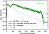 |
Fig. 2. Comparison between our preferred double-peaked 56Ni model plus magnetar (black solid line) and the SN bolometric data from Chen et al. (2024). |
While our model does not explicitly reproduce the steep decline around 270 days, this would effectively mimic a shutdown of the central engine, leaving the radioactive decay as the dominant source. Figure 2 shows an LC with a black solid line where we calibrated the onset of magnetar power suppression (i.e., the magnetar is no longer an energy source by an had oc switch off at 270 d). The transition is rapid but not instantaneous, taking about ∼18 d for the LC to return to the decline rate expected from the nickel decay alone. Similar mechanisms invoking variable thermal energy injection from a magnetar have been proposed to explain other LC morphologies, such as bumps Moriya & Murase (2022), Chugai & Utrobin (2022). Moreover, magnetars and pulsars frequently exhibit erraticspin-down behavior, including sudden spin-down rate variations with no substantial dependence on the spin frequency (Lower et al. 2025). In combination with the spin, the magnetic field might change, leading to a noticeable effect on the magnetar power (Kondić et al. 2011; Torres-Forné et al. 2016).
4. Conclusions
Among the growing diversity of double-peaked SNe, SN 2022jli stands out as a particularly remarkable case. In this work, we have focused on modeling the overall LC as a powerful diagnostic tool to infer the physical parameters of the explosion independently of other observational studies. Our analysis shows that the model relying solely on a double-peaked distribution of 56Ni faces challenges in replicating the observed LC, particularly the sharp decline at late times. Moreover, it requires a total radioactive mass M(56Ni) ≳ 0.35 M⊙, which is high compared to typical core-collapse stripped envelope SNe.
We therefore explored a hybrid energy-source scenario incorporating both radioactive decay and a magnetar as energy sources. In our preferred configuration, most of the total M(56Ni) ≈ 0.15 M⊙ is located in the outer layers of the progenitor to account for the first peak of the LC. The late luminosity reported by Cartier et al. (2024) remains consistent with this estimate.
While the energy input from the magnetar is significantly lower than that of superluminous SNe (e.g., Inserra et al. 2013; Wang et al. 2015), the long spin-down timescale aligns well with the timing of the second peak. The decline from this peak is better reproduced by energy supplied by a magnetar rather than by nickel decay alone. Although the hybrid models are not without limitations, they provide a better overall fit to the observed LC, especially to the pronounced dip between the two peaks. Furthermore, assuming that magnetar power ceases to be efficiently thermalized at ∼270 days, the sharp declining phase up to ∼290 d is well reproduced. Additional observational constraints during the data gap between ∼290 d and ∼400 d will be valuable for ruling out or validating competing models, either through our methods or by studying spectroscopic features (Maeda et al. 2007; Omand & Jerkstrand 2023; Dessart et al. 2012; and subsequent works). Among the scenarios we explored, we conclude that a hybrid model powered by both a double-peaked 56Ni distribution and a magnetar is currently the most plausible explanation for SN 2022jli, although our model does not explain the interesting undulations shown in the LC at late epochs.
The parameters obtained with our model are subject to the assumption that the contribution outside 3750−25 000 Å is small, as suggested by Chen et al. (2024).
We have found that small deviations from n = 3 have a slight effect. Major variations of n were explored by Orellana & Bersten (2020) and Omand & Sarin (2024).
Acknowledgments
This research was partially funded by UNRN PI2020 40B1039, Programa Bilateral de intercambio CSIC-iCOOP del Consejo Superior de Investigaciones Científicas de España, and the support of CONICET through project PIP 112-202001-10034. C.P.G. acknowledges financial support from the Secretary of Universities and Research (Government of Catalonia) and by the Horizon 2020 Research and Innovation Programme of the European Union under the Marie Skłodowska-Curie and the Beatriu de Pinós 2021 BP 00168 program, the support from the Spanish Ministerio de Ciencia e Innovación (MCIN) and the Agencia Estatal de Investigación (AEI) 10.13039/501100011033 under the PID2023-151307NB-I00 SNNEXT project, from Centro Superior de Investigaciones Científicas (CSIC) under the PIE project 20215AT016 and the program Unidad de Excelencia María de Maeztu CEX2020-001058-M, and from the Departament de Recerca i Universitats de la Generalitat de Catalunya through the 2021-SGR-01270 grant.
References
- Aloy, M. Á., & Obergaulinger, M. 2021, MNRAS, 500, 4365 [Google Scholar]
- Anderson, J. P. 2019, A&A, 628, A7 [NASA ADS] [CrossRef] [EDP Sciences] [Google Scholar]
- Bersten, M. C., Benvenuto, O., & Hamuy, M. 2011, ApJ, 729, 61 [NASA ADS] [CrossRef] [Google Scholar]
- Bersten, M. C., Tanaka, M., Tominaga, N., et al. 2013, ApJ, 767, 143 [NASA ADS] [CrossRef] [Google Scholar]
- Bugli, M., Guilet, J., & Obergaulinger, M. 2021, MNRAS, 507, 443 [NASA ADS] [CrossRef] [Google Scholar]
- Cartier, R., Contreras, C., Stritzinger, M., et al. 2024, A&A, submitted [arXiv:2410.21381] [Google Scholar]
- Chen, P., Gal-Yam, A., Sollerman, J., et al. 2024, Nature, 625, 253 [NASA ADS] [CrossRef] [Google Scholar]
- Chevalier, R. A., & Fransson, C. 2008, ApJ, 683, L135 [NASA ADS] [CrossRef] [Google Scholar]
- Chrimes, A. A., Levan, A. J., Fruchter, A. S., et al. 2022, MNRAS, 513, 3550 [NASA ADS] [CrossRef] [Google Scholar]
- Chugai, N. N., & Utrobin, V. P. 2022, MNRAS, 512, L71 [NASA ADS] [CrossRef] [Google Scholar]
- Dessart, L., Hillier, D. J., Li, C., & Woosley, S. 2012, MNRAS, 424, 2139 [NASA ADS] [CrossRef] [Google Scholar]
- Eldridge, J. J., Izzard, R. G., & Tout, C. A. 2008, MNRAS, 384, 1109 [Google Scholar]
- Ertl, T., Woosley, S. E., Sukhbold, T., & Janka, H. T. 2020, ApJ, 890, 51 [CrossRef] [Google Scholar]
- Filippenko, A. V. 1997, ARA&A, 35, 309 [NASA ADS] [CrossRef] [Google Scholar]
- Folatelli, G., Contreras, C., Phillips, M. M., et al. 2006, ApJ, 641, 1039 [NASA ADS] [CrossRef] [Google Scholar]
- Gal-Yam, A. 2017, in Observational and Physical Classification of Supernovae, eds. A. W. Alsabti, & P. Murdin, 195 [Google Scholar]
- Georgy, C., Meynet, G., Walder, R., et al. 2009, A&A, 502, 611 [NASA ADS] [CrossRef] [EDP Sciences] [Google Scholar]
- Gutiérrez, C. P., Bersten, M. C., Orellana, M., et al. 2021, MNRAS, 504, 4907 [CrossRef] [Google Scholar]
- Gutiérrez, C. P., Pastorello, A., Bersten, M., et al. 2022, MNRAS, 517, 2056 [CrossRef] [Google Scholar]
- Hammer, N. J., Janka, H. T., & Müller, E. 2010, ApJ, 714, 1371 [NASA ADS] [CrossRef] [Google Scholar]
- Heger, A., Fryer, C. L., Woosley, S. E., Langer, N., & Hartmann, D. H. 2003, ApJ, 591, 288 [CrossRef] [Google Scholar]
- Inserra, C., Smartt, S. J., Jerkstrand, A., et al. 2013, ApJ, 770, 128 [NASA ADS] [CrossRef] [Google Scholar]
- Kasen, D. 2017, in Unusual Supernovae and Alternative Power Sources, eds. A. W. Alsabti, & P. Murdin, 939 [Google Scholar]
- Kasen, D., & Bildsten, L. 2010, ApJ, 717, 245 [NASA ADS] [CrossRef] [Google Scholar]
- King, A., & Lasota, J.-P. 2024, A&A, 682, L22 [NASA ADS] [CrossRef] [EDP Sciences] [Google Scholar]
- Kondić, T., Rüdiger, G., & Hollerbach, R. 2011, A&A, 535, L2 [NASA ADS] [CrossRef] [EDP Sciences] [Google Scholar]
- Lower, M. E., Karastergiou, A., Johnston, S., et al. 2025, MNRAS, 538, 3104 [Google Scholar]
- Lyman, J. D., Bersier, D., James, P. A., et al. 2016, MNRAS, 457, 328 [Google Scholar]
- Maeda, K., Tanaka, M., Nomoto, K., et al. 2007, ApJ, 666, 1069 [NASA ADS] [CrossRef] [Google Scholar]
- Medin, Z., & Lai, D. 2010, MNRAS, 406, 1379 [NASA ADS] [Google Scholar]
- Metzger, B. D., Thompson, T. A., & Quataert, E. 2007, ApJ, 659, 561 [Google Scholar]
- Modjaz, M., Li, W., Butler, N., et al. 2009, ApJ, 702, 226 [NASA ADS] [CrossRef] [Google Scholar]
- Modjaz, M., Gutiérrez, C. P., & Arcavi, I. 2019, Nat. Astron., 3, 717 [NASA ADS] [CrossRef] [Google Scholar]
- Monard, L. 2022, Transient Name Server Discovery Report, 2022-1198, 1 [Google Scholar]
- Moore, T., Smartt, S. J., Nicholl, M., et al. 2023, ApJ, 956, L31 [NASA ADS] [CrossRef] [Google Scholar]
- Moriya, T. J., Murase, K., et al. 2022, MNRAS, 513, 6210 [NASA ADS] [CrossRef] [Google Scholar]
- Nicholl, M., Guillochon, J., & Berger, E. 2017, ApJ, 850, 55 [NASA ADS] [CrossRef] [Google Scholar]
- Nomoto, K. I., Iwamoto, K., & Suzuki, T. 1995, Phys. Rep., 256, 173 [CrossRef] [Google Scholar]
- Omand, C. M. B., & Jerkstrand, A. 2023, A&A, 673, A107 [NASA ADS] [CrossRef] [EDP Sciences] [Google Scholar]
- Omand, C. M. B., & Sarin, N. 2024, MNRAS, 527, 6455 [Google Scholar]
- Orellana, M., & Bersten, M. C. 2020, BAAA, 61B, 63 [Google Scholar]
- Orellana, M., & Bersten, M. C. 2022, A&A, 667, A92 [NASA ADS] [CrossRef] [EDP Sciences] [Google Scholar]
- Paxton, B., Bildsten, L., Dotter, A., et al. 2011, ApJS, 192, 3 [Google Scholar]
- Piran, T., Nakar, E., Mazzali, P., & Pian, E. 2019, ApJ, 871, L25 [NASA ADS] [CrossRef] [Google Scholar]
- Podsiadlowski, P., Joss, P. C., & Hsu, J. J. L. 1992, ApJ, 391, 246 [Google Scholar]
- Prentice, S. J., Mazzali, P. A., Pian, E., et al. 2016, MNRAS, 458, 2973 [NASA ADS] [CrossRef] [Google Scholar]
- Soderberg, A. M., Berger, E., Page, K. L., et al. 2008, Nature, 453, 469 [NASA ADS] [CrossRef] [Google Scholar]
- Taddia, F., Sollerman, J., Fremling, C., et al. 2018, A&A, 609, A106 [NASA ADS] [CrossRef] [EDP Sciences] [Google Scholar]
- Thompson, C. 2008, ApJ, 688, 499 [NASA ADS] [CrossRef] [Google Scholar]
- Torres-Forné, A., Cerdá-Durán, P., Pons, J. A., et al. 2016, MNRAS, 456, 3813 [Google Scholar]
- Vurm, I., & Metzger, B. D. 2021, ApJ, 917, 77 [NASA ADS] [CrossRef] [Google Scholar]
- Wang, S. Q., Wang, L. J., Dai, Z. G., & Wu, X. F. 2015, ApJ, 799, 107 [NASA ADS] [CrossRef] [Google Scholar]
- Wei, Y.-J., Yang, Y.-P., Wei, D.-M., & Dai, Z.-G. 2024, A&A, 688, A114 [NASA ADS] [CrossRef] [EDP Sciences] [Google Scholar]
- Woosley, S. E. 2010, ApJ, 719, L204 [NASA ADS] [CrossRef] [Google Scholar]
Appendix A: Interaction with circumstellar material
To further investigate the origin of SN 2022jli and given that circumstellar material (CSM) interaction is commonly invoked for some types of core-collapse SNe, we explored the potential contribution from CSM interaction using our code, assuming a stationary wind configuration. For SNe with the explosion date well established, these parameters can be constrained through early-time data modeling. For SN 2022jli, in accordance with the rest of the work, we assumed that the explosion coincides with the discovery date.
Although we did not conduct an thorough parameter space exploration, we performed a set of calculations, including the CSM, to estimate the mass and extent required to reproduce the first peak. We assumed a CSM expanding at a constant velocity of 115 km s−1. For our He11 progenitor model, we find that approximately 2 M⊙ of external material is needed to reach the luminosity level of the first peak and to reproduce an evolution roughly compatible with the first 30 days of the LC. This mass of CSM would extend up to 250 R⊙, i.e. about 50 times the stellar radius. We find that our estimates are broadly consistent with the results of Moore et al. (2023).
While a more detailed exploration of this scenario is beyond the scope of this work, a combined model involving both CSM interaction and magnetar input remains an interesting possibility that justifies further investigation. Importantly, if a specific CSM configuration is adopted, the magnetar parameters required to power the second peak would need to be recalibrated since the total ejected mass would increase in a non-negligible way with respect to the original model.
All Figures
|
Fig. 1. Light curve comparison between the SN observations (gray markers; Chen et al. 2024 bolometric) and the bolometric output from our double-peaked 56Ni distribution model. The inner component of the distribution is varied, while a fixed outer component of the profile is set to provide a reasonable fit for the first maximum of the LC. The model including a magnetar component is shown in magenta. In all the cases, the external enriched 56Ni shell is fixed, and the progenitor is the He11, as detailed in the text. |
| In the text | |
|
Fig. 2. Comparison between our preferred double-peaked 56Ni model plus magnetar (black solid line) and the SN bolometric data from Chen et al. (2024). |
| In the text | |
Current usage metrics show cumulative count of Article Views (full-text article views including HTML views, PDF and ePub downloads, according to the available data) and Abstracts Views on Vision4Press platform.
Data correspond to usage on the plateform after 2015. The current usage metrics is available 48-96 hours after online publication and is updated daily on week days.
Initial download of the metrics may take a while.