© The Authors 2025

1. Introduction

Twenty years ago, the High Energy Stereoscopic System (H.E.S.S.) detected orbitally modulated, very-high-energy (VHE; 100 GeV ≲ ϵ ≲ 100 TeV) emission and photons with energies reaching ϵ ∼ 30 TeV from LS 5039 (Aharonian et al. 2006a), a high-mass binary considered to be a likely GeV-emitting microquasar at the time (Paredes et al. 2000). Some years later, Fermi confirmed the source to be a GeV emitter (Abdo et al. 2009; Hadasch et al. 2012), and a re-analysis of MeV data strengthened previous evidence of detection in the MeV range (Collmar & Zhang 2014). This information was complemented by soft and hard X-ray observations, which found an orbital light curve similar to that in TeV (e.g., Bosch-Ramon et al. 2005; Hoffmann et al. 2009; Takahashi et al. 2009), and to that hinted by the MeV data re-analysis. The High-Altitude Water Cherenkov Observatory (HAWC) has recently detected the source up to ϵ ≈ 200 TeV, reaching the photon ultra-high-energy (UHE; ϵ > 100 TeV) range, with a spectral energy distribution (SED) ∝ϵ^−0.8 that shows no evidence of a high-energy cut-off (Alfaro et al. 2025). HAWC has also found 2.7σ evidence of orbital variability in the 40 − 118 TeV range, and 2.2σ evidence above 100 TeV. Furthermore, the emission detected around the inferior conjunction of the compact object (INFC; orbital phase range 0.45 − 0.9) reaches 208 TeV, whereas around the superior conjunction (SUPC) the emission reaches 118 TeV, which also suggests variability above 100 TeV.

LS 5039 was initially considered to be a microquasar due to the presence of X-ray accretion features and radio jets (Ribó et al. 1999; Paredes et al. 2000). However, several authors proposed that this system may host a young pulsar instead (Martocchia et al. 2005; Dubus 2006b), as in the case of PSR B1259-63/LS2883, which is also a TeV-emitting binary (Johnston et al. 1992; Aharonian et al. 2005). In addition, it was found that the previously found X-ray accretion features were likely to be background contamination due to the poor angular resolution of RXTE (Ribó et al. 1999; Bosch-Ramon et al. 2005). However, while a pulsar-star wind collision scenario is generally accepted to be behind the nonthermal (NT) emission in PSR B1259-63/LS2883 (e.g., Tavani & Arons 1997; Khangulyan et al. 2007; see however Yi & Cheng 2017), in LS 5039 a microquasar scenario cannot yet be fully discarded. The compact object mass has not been ascertained (Casares et al. 2005), the presence of pulsations is controversial (Yoneda et al. 2020; Kargaltsev et al. 2023; Makishima et al. 2023), and some accretion modes may not yield prominent features such as thermal emission and spectroscopic lines (Okazaki et al. 2008; Barkov & Khangulyan 2012). More exotic scenarios have been discussed as well, such as a young magnetar, prompted by the hint of pulsations with a period of ≈9 s found in X-rays (Yoneda et al. 2020). Such an object, however, seems to be at odds with the absence of a conspicuous supernova remnant surrounding the source (Ribó et al. 2002; Moldón et al. 2012), and assessing its feasibility needs further theoretical development (Bosch-Ramon & Barkov, in prep.). Therefore, the debate about the processes yielding the NT emission in LS 5039 remains far from being solved, a debate that is tightly connected to other similar systems. In particular, in LS I +61 303, which presents evidence for 269 ms radio pulsations (Weng et al. 2022) and thus disfavors the microquasar scenario (see however Jaron et al. 2024), the question of the origin of the NT emission is still open (e.g., a colliding-wind model vs. a transitional – magnetar-like – pulsar scenario; e.g., Dubus 2006b; Papitto et al. 2012).

Despite the puzzles yet to be solved, combining data and theory has helped to reach some conclusions on the properties of the accelerator and the NT emitter in LS 5039. For instance, the multiwavelength NT behavior of LS 5039, and in particular its gamma-ray orbital variability, strongly suggest inverse Compton (IC) scattering of stellar photons as the origin of this emission (e.g., Khangulyan et al. 2008; Dubus et al. 2008; Takahashi et al. 2009). It is worth noting that HAWC results match the behavior found by H.E.S.S. at an overlapping energy range well, so a different mechanism for the UHE emission seems unlikely. Moreover, the modest mass-loss rate of the stellar companion (Casares et al. 2005) further strengthens that hypothesis, as luminous proton-proton emission or relativistic Bremsstrahlung would require an unrealistic energy budget for either protons or electrons, respectively. In addition, the hard photon local fields are too diluted for efficient photo-meson production (Bosch-Ramon & Khangulyan 2009). Khangulyan et al. (2008) also showed that the detection of 30 TeV photons by H.E.S.S. favored an efficient accelerator located in the periphery of the binary to soften the strong acceleration rate requirements, but not far from it due to the presence of variability. Similar conclusions were also reached in Bosch-Ramon et al. (2007) and Bosch-Ramon et al. (2008b) for the X-ray and the VHE emitter, respectively, using arguments based on X-ray absorption and gamma-ray reprocessing. These articles also suggested that this class of scenario was more compatible with a jet-like structure, although an alternative conclusion about the X-ray emitter structure was derived by Szostek & Dubus (2011), who proposed an extended emitting region with a size similar to the system semimajor axis (a), interpreting it as the star-pulsar wind colliding region. Moreover, theoretical studies of the star-pulsar wind interaction along the orbit also predicted the acceleration of particles outside the binary due to a combination of the Coriolis force and the slow stellar wind, which should trigger a strong lateral shock on the pulsar wind as it propagates away from the orbiting binary (the Coriolis shock; e.g., Bosch-Ramon & Barkov 2011; Bosch-Ramon et al. 2012). Numerical studies also showed that the magnetic field could introduce further structure to the two-wind interaction region on the scales of the binary system (e.g., Bogovalov et al. 2019; Barkov et al. 2024).

In this work, we aimed to improve our knowledge of the NT accelerator and emitter in LS 5039 by exploring the consequences of HAWC observational results using analytical tools. This analysis, approximate but suitable for this source due to the large uncertainties involved, is based on the spectral and variability properties of the UHE emission and is conducted within the framework of IC scattering off stellar photons. We took ϵ = 100 TeV as the reference photon energy to study the orbital variability, a compromise between assuming that the modulation is only real up to ϵ ∼ 40 TeV, or that it actually goes beyond ∼100 TeV as INFC photons reach ≈208 TeV while SUPC photons reach just ≈118 TeV, and Alfaro et al. 2025 found 2.2σ evidence of orbital variability above 100 TeV. The present work strengthens the conclusions of Khangulyan et al. (2008), gets deeper into the global implications for the emitter and the accelerator, and proposes an acceleration mechanism based on Derishev et al. (2003) and Derishev & Aharonian (2012). The paper is organized as follows. The emitting and the acceleration regions are discussed in Sects. 2 and 3, respectively, and the suggested model is proposed in Sect. 4. We conclude with Sect. 5.

2. The UHE photon emitter

While the H.E.S.S. observational results presented in Aharonian et al. (2006a) already put important limits on the properties of the VHE emitter and the associated accelerator in LS 5039 (e.g., Khangulyan et al. 2008), the recent HAWC results have yielded tighter constraints, as can be seen in the discussion carried out by Alfaro et al. (2025) in the context of the leptonic scenario. This is particularly true if the emission indeed reaches higher energies around the INFC than around the SUPC. To get deeper into the consequences of the HAWC results, we start by studying the UHE emitting region adopting the framework of stellar IC for the reasons given above. For those aspects concerning IC scattering, we refer to Khangulyan et al. (2014). As mentioned in Sect. 1, we took ϵ = 100 TeV as the photon energy reference. To produce 100 TeV photons, IC scattering off stellar photons with ϵ_* ≈ 10 eV takes place deep in the Klein-Nishina regime (KN; i.e., E ≫ m_e²c⁴/ϵ_⋆), and requires electrons with E ≈ 120 TeV.

Anisotropic IC scattering and γγ absorption represent two geometrical factors that may influence the orbital phase dependence of the gamma-ray emission, but their influence is strongly suppressed in the UHE regime. Thus, the orbital UHE variability is caused by one or several of these other factors changing along the orbit: hydrodynamics (i.e., escape, adiabatic losses, or heating); intrinsic emission beaming (i.e., Doppler boosting or an anisotropic electron angular distribution); and IC target density. All these effects (including the minor geometric ones) can only be present if the emitter size (R_em) is not significantly larger than a, as otherwise orbital variability would be washed out. Moreover, the mean free path, λ, of the highest energy particles in the emitter (at least equal to their gyroradius r_g = E/qℬ_em, where q is the absolute value of the particle charge and ℬ_em is the magnetic field strength in the emitter) should fulfill (λ/r_g)r_g ≲ R_em ≲  a. Thus, electron confinement requires an emitter magnetic field

$$\begin{array}{c}\hfill {\mathcal{B}}_{\mathrm{em}}\gtrsim 0.2\left(\frac{\lambda }{r_{\mathrm{g}}}\right)\left(\frac{E}{120\mathrm{TeV}}\right){\left(\frac{R_{\mathrm{em}}}{a}\right)}^{-1}\mathrm{G},\end{array}$$(1)

for a = 2.2 × 10¹² cm (Casares et al. 2005).

Further constraints can be derived from the spectral slope in the UHE regime. Since for 120 TeV electrons the KN parameter reaches Eϵ_⋆/m_e²c⁴ ∼ 5 × 10³, one can adopt the asymptotic relation between the photon and the electron spectra. In particular, the gamma-ray differential distribution $d{N}_{ϵ}/dϵ\propto {ϵ}^{-2.83\pm 0.{09}_{-0.05}^{+0.02}}$ around INFC (Alfaro et al. 2025) requires an emitting electron spectrum similar to dN/dE ∝ E⁻² within uncertainties. Synchrotron losses modify the electron injection spectrum (dQ/dE = dN_inj/dEdt) as follows:

$$\begin{array}{c}\hfill dQ/dE\propto E^{-r}\to dN/dE\propto E^{-(r+1)}\mathrm{for}r\gtrsim 1;\mathrm{and}\end{array}$$(2)

$$\begin{array}{c}\hfill dQ/dE\propto E^{-r}\to dN/dE\propto E^{-2}\mathrm{for}r\lesssim 1.\end{array}$$(3)

Thus, considering that dN/dE ∝ E⁻², one reaches the conclusion that either dQ/dE ∝ E⁻¹ or harder, or dQ/dE ∝ E⁻² and the magnetic field is low enough to avoid dominant synchrotron losses. One can compare the synchrotron timescale and the shortest possible escape (or adiabatic) loss time, which are

$$\begin{array}{c}\hfill t_{\mathrm{sync}}\approx 3.3{\left(\frac{E}{120\mathrm{TeV}}\right)}^{-1}{\left(\frac{{\mathcal{B}}_{\mathrm{em}}}{1\mathrm{G}}\right)}^{-2}\mathrm{s}\mathrm{and}\end{array}$$(4)

$$\begin{array}{c}\hfill t_{\mathrm{esc}}\sim R_{\mathrm{em}}/c\approx 73\left(\frac{R_{\mathrm{em}}}{a}\right)\mathrm{s},\end{array}$$(5)

respectively (likely, v_em ∼ c as particles are marginally confined in the region). Assuming dominant escape (or adiabatic) losses, one obtains the constraint

$$\begin{array}{c}\hfill {\mathcal{B}}_{\mathrm{em}}\lesssim 0.2{\left(\frac{E}{120\mathrm{Tev}}\right)}^{-1/2}{\left(\frac{R_{\mathrm{em}}}{a}\right)}^{-1/2}\mathrm{G};\end{array}$$(6)

at E = 120 TeV, only for R_em ∼ a is this marginally compatible with Eq. (1). If orbital variability were limited to ϵ ≲ 40 TeV, meaning a reference electron energy of E ≈ 50 TeV, negligible synchrotron losses and the condition λ ≲ a would imply that λ ≲ 3 r_g, which is still a very strong confinement condition. Therefore, assuming negligible synchrotron losses in the emitter is narrowly consistent with r_g ≲ R_em ≲ a and seems to be disfavored (implying a very hard dQ/dE; see Sect. 4, however).

To provide further context, one can derive an (conservative) upper limit on the magnetic field strength in the emitter:

$$\begin{array}{c}\hfill {\mathcal{B}}_{\mathrm{em}}\lesssim \sqrt{\frac{L_{\mathrm{w}}}{v_{\mathrm{em}}{R}_{\mathrm{em}}^2}}\approx 3{\left(\frac{L_{\mathrm{NT}}}{{10}^{36}\mathrm{erg}/\mathrm{s}}\right)}^{1/2}{\left(\frac{v_{\mathrm{em}}}{c}\right)}^{-1/2}{\left(\frac{R_{\mathrm{em}}}{a}\right)}^{-1}\mathrm{G},\end{array}$$(7)

where v_em is the emitting flow velocity and a spherical geometry is assumed. The equation was derived taking into account that the Poynting flux cannot overcome the total power of the source (L_w), and that this power minimum value is that required to feed the NT emission in LS 5039 (i.e., L_NT ≳ 10³⁶ erg s⁻¹ from the overall MeV-peaked SED; Collmar & Zhang 2014). If electrons escaped to the stellar wind region and radiated there, they would find a magnetic field:

$$\begin{array}{c}\hfill {\mathcal{B}}_{\mathrm{em}}\lesssim \sqrt{\frac{L_{\mathrm{w},\ast }}{v_{\ast }{R}_{\mathrm{em}}^2}}\approx 11{\left(\frac{{\dot{M}}_{\ast }}{{10}^{-7}{\mathrm{M}}_{\odot }/\mathrm{yr}}\right)}^{1/2}{\left(\frac{v_{\ast }}{2000\mathrm{km}/\mathrm{s}}\right)}^{-1/2}{\left(\frac{R_{\mathrm{em}}}{a}\right)}^{-1}\mathrm{G},\end{array}$$(8)

where L_w, * is the stellar wind power, and the wind mass-loss rate (Ṁ_∗) and velocity (v_*) were normalized to values typical for LS 5039 (Casares et al. 2005). These estimates show that, at the energies considered (E ≳ 50 TeV), ℬ_em values well below equipartition can already lead to dominant synchrotron cooling.

It is informative to derive the synchrotron luminosity of the electrons behind the UHE emission (L_sync, UHE) under the assumption that R_em ∼ a. We focused on photon energies ϵ ≳ 40 TeV (E ≳ 50 TeV), for which the INFC luminosity detected by HAWC is L_HAWC ≈ 2.1 × 10³² erg s⁻¹ at a 2 kpc distance. The synchrotron luminosity is determined by the ratio of the relevant cooling times:

$$\begin{array}{c}\hfill L_{\mathrm{sync},\mathrm{UHE}}\sim \frac{t_{\mathrm{KN}}}{t_{\mathrm{sync}}}{L}_{\mathrm{HAWC}}\sim 3\times {10}^{33}{\left(\frac{{\mathcal{B}}_{\mathrm{em}}}{0.4\mathrm{G}}\right)}^2{\mathrm{erg}\mathrm{s}}^{-1},\end{array}$$(9)

where t_KN is the KN IC timescale (Khangulyan et al. 2014):

$$\begin{array}{c}\hfill t_{\mathrm{KN}}\sim 7\times {10}^2{\left(\frac{E}{50\mathrm{TeV}}\right)}^{0.7}{\left(\frac{max[R_{\mathrm{em}},a]}{a}\right)}^2\mathrm{s},\end{array}$$(10)

for the star luminosity and temperature (Casares et al. 2005), and imposing a minimum distance to the star of a (around the location of the compact object). Adopting ℬ_em ∼ 3 G, for instance, L_sync, UHE is ∼2 × 10³⁵ erg s⁻¹ and the energy of the synchrotron photons from electrons with E ≳ 50 TeV is ϵ ≳ 500 MeV¹. As shown above, dN/dE ∝ E⁻², which implies a synchrotron SED ∝ϵ^1/2 at ϵ ≳ 500 MeV. This SED is harder than, and the derived L_sync, UHE-value similar to, what was observed at those energies (e.g., Hadasch et al. 2012; Collmar & Zhang 2014), which point to an electron component dominating at lower energies that is different from that producing the UHE emission. This also means that, since under dominant synchrotron losses L_NT, UHE ∼ L_sync, UHE, in that case L_NT, UHE must be lower than ∼2 × 10³⁵ erg s⁻¹ (i.e. ℬ_em < 3 G) not to violate the observed GeV fluxes.

For the case with negligible synchrotron losses (e.g., ℬ_em < 0.4 G for E = 50 TeV), escape (adiabatic) losses most likely dominate over any radiative cooling (including IC), and thus one obtains (for R_em ∼ a)

$$\begin{array}{c}\hfill L_{\mathrm{NT},\mathrm{UHE}}\sim \frac{t_{\mathrm{KN}}}{t_{\mathrm{esc}}}{L}_{\mathrm{HAWC}}\sim 3\times {10}^{33}{\mathrm{erg}\mathrm{s}}^{-1},\end{array}$$(11)

which implies that L_NT, UHE ≪ L_NT and again a different electron component should be behind the brighter emission at lower energies. Increasing L_NT, UHE would require a R_em ≪ a, which is not possible if ℬ_em is to be low while simultaneously λ ≲ R_em (see, however, Sect. 4).

3. The accelerator

Since accelerated electrons may escape the accelerator into a different region where they would produce most of the UHE emission, the properties of the accelerator must be derived separately. Strong constraints on the accelerator magnetic field (ℬ_acc) can also be obtained by considering λ ≲ R_acc ≲ a, with R_acc being the accelerator size. The acceleration timescale for electrons of energy E, t_acc, was defined as

$$\begin{array}{c}\hfill t_{\mathrm{acc}}\sim {\eta }_{\mathrm{acc}}\frac{r_{\mathrm{g}}(E)}{c}={\eta }_{\mathrm{acc}}\frac{E}{q{\mathcal{B}}_{\mathrm{acc}}c},\mathrm{with}{\eta }_{\mathrm{acc}}>1.\end{array}$$(12)

Here, ℬ_acc refers to the component of the electromagnetic field doing the acceleration work, which is in fact the electric field depending on the frame of reference or the acceleration mechanism considered.

The constraint λ ≲ R_acc ≲ a implies that, similarly to ℬ_em,

$$\begin{array}{c}\hfill {\mathcal{B}}_{\mathrm{acc}}\gtrsim 0.2\left(\frac{\lambda }{r_{\mathrm{g}}}\right)\left(\frac{E}{120\mathrm{TeV}}\right){\left(\frac{R_{\mathrm{acc}}}{a}\right)}^{-1}\mathrm{G}.\end{array}$$(13)

Moreover, the condition t_acc ≲ t_sync must be fulfilled for electrons to be able to reach an energy E, so:

$$\begin{array}{c}\hfill t_{\mathrm{acc}}\lesssim t_{\mathrm{sync}}\to {\mathcal{B}}_{\mathrm{acc}}\lesssim 0.2{\left(\frac{{\eta }_{\mathrm{acc}}}{1}\right)}^{-1}{\left(\frac{E}{120\mathrm{Tev}}\right)}^{-2}\mathrm{G};\end{array}$$(14)

for R_acc ∼ a, this is marginally compatible only with λ ∼ r_g and η_acc ∼ 1 at E = 120 TeV, while at E = 50 TeV, λ ≲ 3r_g and η_acc ≲ 3 are required, which are still quite extreme restrictions on particle confinement and the acceleration rate, respectively. All this was already discussed in Khangulyan et al. (2008) in the context of H.E.S.S. results (see, e.g., Fig. 2 in that paper), but HAWC results strengthen the observational constraints. We remark that few known astrophysical sources present such demanding requirements for both t_acc and λ. Nonetheless, if synchrotron losses and particle confinement could be decoupled, the requirements would relax significantly. In the next section, we consider an acceleration model based on Derishev et al. (2003) and Derishev & Aharonian (2012) in which this may happen.

4. Acceleration model

Synchrotron cooling and confinement decouple when particles that are roughly isotropic in the laboratory frame (LF) are immersed in a magnetized relativistic outflow. Under these conditions, the flow frame (FF) magnetic field is able to deflect the particles enough for them to acquire a large amount of energy in the LF (as demonstrated in Sects. 4.1 and 4.2), while the rate of synchrotron cooling in the FF is significantly reduced (as shown in Sect. 4.3). The presence of a bright stellar companion provides a way to bring relativistic particles into the relativistic outflow: LS 5039 is optically thick for gamma rays with energies between ∼10 GeV and 10 TeV interacting with stellar photons on binary scales, so secondary e^± pairs (secondaries hereafter) are expected to be injected within the binary (e.g., Dubus 2006a; Aharonian et al. 2006b), and thus within the outflow produced by the compact object (Derishev & Aharonian 2012). These secondaries, which constitute the seed particles for the acceleration process, are mostly created with energies in the range ∼10 − 100 GeV, depending on their injection location in the system with respect to the gamma-ray emitter (Bosch-Ramon et al. 2008a). Secondaries could also be created in the local NT emitter photon fields², although we focus on those from γγ absorption in the stellar photon field because they reach the highest energies once accelerated.

To derive a simple analytical estimate of the maximum achievable energies in the described scenario, we assumed a planar wind moving with bulk speed v_w carrying a perpendicular magnetic field that terminates at a distance R_acc from its origin. We assumed that the wind is ultrarelativistic, $\mathrm{\Gamma }=1/\sqrt{1-{\beta }_{\mathrm{w}}^2}\gg 1$, where β_w = v_w/c. The wind termination would occur in a shock caused by the presence of the stellar wind. Most of the injected secondaries, which are assumed to have an energy E₀, initially move in the FF within a cone of half opening angle ∼1/Γ against the wind. Once injected, the secondaries gyrate around the magnetic field, which is ℬ_acc and ${\mathcal{B}}_{\mathrm{acc}}^{\prime }={\mathcal{B}}_{\mathrm{acc}}/\mathrm{\Gamma }$ in the LF and the FF, respectively (primed quantities are in the FF). The secondaries injected in the direction opposite to the flow motion have the highest energy in the FF: E′=(1 + β_w)ΓE₀ ≈ 2ΓE₀, and a gyroradius

$$\begin{array}{c}\hfill r_{\mathrm{g}}^{\prime }=\frac{E^{\prime }}{q{\mathcal{B}}_{\mathrm{acc}}^{\prime }}=\frac{(1+{\beta }_{\mathrm{w}}){\mathrm{\Gamma }}^2{E}_0}{q{\mathcal{B}}_{\mathrm{acc}}}\approx 2{\mathrm{\Gamma }}^2{r}_{\mathrm{g},0},\end{array}$$(15)

where both E′ and r′_g are constant in the FF in a planar wind. Most of the secondaries injected with energy E₀, if moving isotropically in the LF, have similar though slightly lower E′ values. For simplicity, we assumed no electric field in the wind FF, that is, the plasma has infinite conductivity. A sketch of the process from the point of view of both the FF and the LF is shown in Fig. 1.

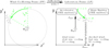Fig. 1. Sketch of the acceleration process. An electron gyrates in the XY plane in the FF (left) following a circular trajectory (green line), whereas in the LF (right) it gets quickly accelerated initially by the electric field of the wind, and deflected towards the wind direction of motion. The wind moves in the X direction, and the FF and LF magnetic field and the LF electric field are perpendicular to the flow motion.

Equation (15) provides an illustrative way to find an upper limit for the maximum change in the particle energy in the LF. If a particle gyrates for exactly half an orbit starting from an initial orientation against the wind, then its maximum vertical displacement is 2r′_g in the FF; in the LF, the maximum particle vertical displacement is 2r′_g as well. Since in the LF the electric field, ℰ_acc, is also perpendicular to the wind bulk speed, the maximum possible energy gain is thus

$$\begin{array}{c}\hfill \mathrm{\Delta }{E}_{\max }=2r_{\mathrm{g}}^{\prime }q{\mathcal{E}}_{\mathrm{acc}}=2(1+{\beta }_{\mathrm{w}}){\mathrm{\Gamma }}^2{E}_0{\beta }_{\mathrm{w}}\approx 4{\mathrm{\Gamma }}^2{E}_0{\beta }_{\mathrm{w}},\end{array}$$(16)

where we used the relation between the electric and the magnetic field strengths ℰ_acc = β_wℬ_acc.

4.1. Maximum energy

With no acceleration size constraints, a particle injected in the direction against the wind bulk velocity keeps gyrating, and its energy in the LF follows a periodic pattern between E₀ and E₀ + ΔE_max. The larger the E₀, the larger the potential drop the particle probes, but the longer the time it requires to gyrate. Therefore, particles can only reach their possible maximum energy if their trajectories are confined within the unshocked wind while they complete half an orbit turn. To determine the maximum energy for particles that cannot gyrate half an orbit before reaching the wind termination shock, one needs to solve the particle motion equation in the wind zone accounting for its size and geometry. This equation can be solved either in the LF or in the FF, and each of these systems has its own advantages: the accelerator size constraints are more clearly defined in the LF; however, solving the particle motion under a uniform magnetic field is trivial in the FF. Therefore, in this work we analyzed the particle gyration angle in the FF and then applied a Lorentz transformation to the LF while taking into account the accelerator size constraint in that frame. This is equivalent to solving the equations of motion directly in the LF. For the sake of completeness, a brief discussion of the effect of the Lorentz force in the LF is also provided in Sect. 4.2.

The energy acquired in the LF by the secondaries, which are ultrarelativistic, can be derived from

$$\begin{array}{c}\hfill E=\mathrm{\Gamma }(1-{\beta }_{\mathrm{w}}cos{\theta }^{\prime })E^{\prime }\approx 2{\mathrm{\Gamma }}^2(1-{\beta }_{\mathrm{w}}cos{\theta }^{\prime })E_0,\end{array}$$(17)

where θ′ is the angle by which the particle is deflected in the FF. At the moment of the particle injection, θ′ = 0 and the particle moves in the direction opposite to the wind bulk speed. As shown in Fig. 1, in the FF, the deflection angle, θ′, is equal to the polar angle swept by the particle. The angle θ corresponds to the angle θ′ in the LF (see in Fig. 1), and both angles are related through a Lorentz transformation:

$$\begin{array}{c}\hfill tan\theta =\frac{v^{\prime }sin{\theta }^{\prime }}{\mathrm{\Gamma }(v^{\prime }cos{\theta }^{\prime }-v_{\mathrm{w}})},\end{array}$$(18)

where v and v′ are particle speeds in the LF and FF, respectively, and we accounted for the way these angles are defined (v′_x = −v′ cos θ′, v′_y = −v′ sin θ′, v_x = −v cos θ, and v_y = −v sin θ).

The increase of the particle energy in Eq. (17) is consistent with Eq. (16) as the particle displacement in the direction of the LF electric field is r′_g(1 − cos θ′). The corresponding change of energy is thus

$$\begin{array}{c}\hfill \mathrm{\Delta }E=r_{\mathrm{g}}^{\prime }(1-cos{\theta }^{\prime })q{\mathcal{E}}_{\mathrm{acc}}=(1+{\beta }_{\mathrm{w}}){\mathrm{\Gamma }}^2{E}_0{\beta }_{\mathrm{w}}(1-cos{\theta }^{\prime }),\end{array}$$(19)

which is the same as Eq. (16) when θ′=π.

The maximum angle θ′ for which the particle is still confined in the wind zone can be obtained from the relation between the distance along the X axis in the LF, x, and in the FF, x′:

$$\begin{array}{c}\hfill x=\mathrm{\Gamma }(x^{\prime }(t^{\prime })+{\beta }_{\mathrm{w}}c{t}^{\prime }).\end{array}$$(20)

In the present scenario and setting the origin of coordinates at the place and moment of the injection of the secondary particle, one has

$$\begin{array}{c}\hfill x^{\prime }=r_{\mathrm{g}}^{\prime }cos({\theta }^{\prime }+\pi /2)=-r_{\mathrm{g}}^{\prime }sin{\theta }^{\prime },\end{array}$$(21)

and θ′=v′t′/r′_g. In the FF, the particle moves along a circular trajectory while it remains in the wind zone. The three-dimensional shape of this region might be very complicated (in particular, pulsar winds can be strongly anisotropic; see, e.g., Bogovalov & Khangoulian 2002), so for simplicity we introduced the accelerator size constraint through a parameter with length dimension, R_acc, linked to the radius of the wind termination shock. The particle is considered to be within the wind zone for −R_acc ≤ x ≤ R_acc.

For relatively small E₀ values (e.g., ≲10 MeV for Γ ∼ 10³), secondaries gyrate up to θ′≳π/2, and Eq. (17) yields E ∼ Γ²E₀ (see Eq. (16) above). For the higher E₀ values given above though (∼10 − 100 GeV), θ′ can be ≪1. In that case, we adopted a third order Taylor expansion:

$$\begin{array}{c}\hfill sin{\theta }^{\prime }\approx {\theta }^{\prime }-{\theta }^{\prime 3}/6,cos{\theta }^{\prime }\approx 1-{\theta }^{\prime 2}/2,\end{array}$$(22)

which in fact yields results correct within ∼10% even for θ′∼1.

From Eqs. (20), (21) and (22), the first order Taylor expansion of β_w ≈ 1 − 1/2Γ², the t′-θ′ relation, and the fact that in the present case 1/(1 − (v′/c)²)^1/2 ≫ Γ, we derived for x(θ′)

$$\begin{array}{c}\hfill x=\mathrm{\Gamma }{r}_{\mathrm{g}}^{\prime }{\theta }^{\prime }(-\frac{1}{2{\mathrm{\Gamma }}^2}+\frac{{\theta }^{\prime 2}}{6}).\end{array}$$(23)

Since the acceleration cycle ends when the particle reaches x = R_acc > 0, which implies $\theta \prime >\sqrt{3}/\mathrm{\Gamma }$, we can approximate the gyration angle by neglecting the $\mathcal{O}(1/{\mathrm{\Gamma }}^2)$ term as

$$\begin{array}{c}\hfill {\theta }^{\prime }\approx {\mathrm{\Gamma }}^{-1}{\left(\frac{3E_{\mathrm{H}}}{E_0}\right)}^{1/3},\end{array}$$(24)

where $E_{\mathrm{H}}=q{\mathcal{B}}_{\mathrm{acc}}x=q{\mathcal{B}}_{\mathrm{acc}}{R}_{\mathrm{acc}}$ (Hillas limit). This equation together with Eqs. (17) and (22) yields the maximum attainable energy:

$$\begin{array}{c}\hfill E_{\max }\approx 2.1E_{\mathrm{H}}{\left(\frac{E_0}{E_{\mathrm{H}}}\right)}^{1/3}.\end{array}$$(25)

Assuming a radial wind and a toroidal ℬ_acc, and taking the wind Poynting flux to be a fraction η_B of the ultrarelativistic wind total power L_w, we obtained ${\mathcal{B}}_{\mathrm{acc}}{R}_{\mathrm{acc}}={({\eta }_{\mathrm{B}}{L}_{\mathrm{w}}/c)}^{1/2}$ and

$$\begin{array}{c}\hfill E_{\max }\approx 200{\left(\frac{{\eta }_{\mathrm{B}}{L}_{\mathrm{w}}}{3\times {10}^{36}\mathrm{erg}/\mathrm{s}}\right)}^{1/3}{\left(\frac{E_0}{100\mathrm{GeV}}\right)}^{1/3}\mathrm{TeV},\end{array}$$(26)

similar to those required to explain HAWC observations. Higher energies could be achieved for larger E₀ values, but the number of secondaries strongly diminishes well above 100 GeV. We note that, for a final $\theta \prime <\sqrt{3}/\mathrm{\Gamma }$, x in Eq. (23) is negative and E barely grows above E₀. This applies in the unlikely event that E₀ approaches E_H, so particles escape almost undeflected in the FF.

4.2. Laboratory frame description

The efficiency of the acceleration process can also be illustrated from the point of view of the LF. Namely, the Lorentz force equation (we focus here on an electron with charge −q),

$$\begin{array}{c}\hfill \dot{\mathit{p}}=-q({\mathcal{E}}_{\mathrm{acc}}+\frac{\mathit{v}}{c}\times {\mathcal{B}}_{\mathrm{acc}}),\end{array}$$(27)

can be directly linked to the energy gain rate, Ė. First, E is related to the relativistic three-momentum vector p through

$$\begin{array}{c}\hfill E^2=m^2{c}^4+c^2{\mathit{p}}^2.\end{array}$$(28)

If one derives in time both sides of Eq. (28), it yields

$$\begin{array}{c}\hfill E\dot{E}=c^2\mathit{p}\dot{\mathit{p}},\end{array}$$(29)

and taking into account that pc² = vE, one can write (see, e.g., Landau & Lifshitz 1971)

$$\begin{array}{c}\hfill \dot{E}=\frac{c^2\mathit{p}}{E}\dot{\mathit{p}}=\mathit{v}\dot{\mathit{p}}.\end{array}$$(30)

Using this relation and ${\mathcal{E}}_{\mathrm{acc}}=-{\mathit{\beta }}_{\mathrm{w}}\mathbf{\times }{\mathcal{B}}_{\mathrm{acc}}$ in Eq. (27), one obtains

$$\begin{array}{c}\hfill \dot{E}=\mathit{v}\dot{\mathit{p}}=q\mathit{v}({\mathit{\beta }}_{\mathrm{w}}\times {\mathcal{B}}_{\mathrm{acc}}-\frac{\mathit{v}}{c}\times {\mathcal{B}}_{\mathrm{acc}}),\end{array}$$(31)

and since $\mathit{v}({\mathit{\beta }}_{\mathrm{w}}\times {\mathcal{B}}_{\mathrm{acc}})=v{\beta }_{\mathrm{w}}{\mathcal{B}}_{\mathrm{acc}}sin\theta$ and $\mathit{v}((\mathit{v}/c)\times {\mathcal{B}}_{\mathrm{acc}})=0$,

$$\begin{array}{c}\hfill \dot{E}=qv{\beta }_{\mathrm{w}}{\mathcal{B}}_{\mathrm{acc}}sin\theta \approx q{\mathcal{B}}_{\mathrm{acc}}csin\theta .\end{array}$$(32)

From this expression it can be seen that the most efficient acceleration occurs when θ ≈ π/2, which in the FF corresponds to cos θ′−β_w ≈ 0, i.e., when θ′≈1/Γ (although, as already explained, particles gain most of their LF energy when $\theta \prime >\sqrt{3}/\mathrm{\Gamma }$).

Equation (32) can be computed using the relation $\theta \prime \approx {(3q{\mathcal{B}}_{\mathrm{acc}}c/E_0{\mathrm{\Gamma }}^3)}^{1/3}{t}^{1/3}$ obtained from the Lorentz transformation for time:

$$\begin{array}{c}\hfill t=\mathrm{\Gamma }(t^{\prime }+{\beta }_{\mathrm{w}}\frac{x^{\prime }}{c}).\end{array}$$(33)

Using Eq. (18) in the limits 1/Γ ≲ θ′≪1 and v′≈v_w ≈ c one obtains

$$\begin{array}{c}\hfill sin\theta \approx \frac{2}{\mathrm{\Gamma }{\theta }^{\prime }};\mathrm{i}.\mathrm{e}.sin\theta \approx 2{\left(\frac{E_0}{3q{\mathcal{B}}_{\mathrm{acc}}c}\right)}^{1/3}{t}^{-1/3}.\end{array}$$(34)

Using this last expression, Eq. (32) can be integrated in t yielding

$$\begin{array}{c}\hfill E\approx 3q{\mathcal{B}}_{\mathrm{acc}}c{\left(\frac{E_0}{3q{\mathcal{B}}_{\mathrm{acc}}c}\right)}^{1/3}{t}^{2/3}.\end{array}$$(35)

For t ≈ R_acc/c, it turns out that the above estimate for the particle energy E is equal to E_max in Eq. (25), as expected from the equivalence of both approaches.

4.3. Synchrotron losses

Synchrotron losses are negligible in the discussed scenario as the synchrotron timescale in the FF,

$$\begin{array}{c}\hfill t_{\mathrm{sync}}^{\prime }\approx 200\left(\frac{\mathrm{\Gamma }}{{10}^3}\right){\left(\frac{E_0}{100\mathrm{GeV}}\right)}^{-1}{\left(\frac{{\mathcal{B}}_{\mathrm{acc}}}{100\mathrm{G}}\right)}^{-2}\mathrm{s},\end{array}$$(36)

is much longer than t′ for typical parameter values:

$$\begin{array}{c}\hfill t^{\prime }\approx 10{\left(\frac{R_{\mathrm{acc}}}{{10}^{11}\mathrm{cm}}\right)}^{1/3}{\left(\frac{E_0}{100\mathrm{GeV}}\right)}^{2/3}{\left(\frac{\mathrm{\Gamma }}{{10}^3}\right)}^{-1/3}{\left(\frac{{\mathcal{B}}_{\mathrm{acc}}}{100\mathrm{G}}\right)}^{-2/3}\mathrm{s};\end{array}$$(37)

the normalization ℬ_acc value of 100 G corresponds to the fiducial values of the wind parameters adopted in Sect. 4.1 and η_B = 1. Therefore, ℬ_acc can be high in the lab frame but the accelerated secondaries mostly radiate via IC while they are confined to the ultrarelativistic wind; t′_sync can become < t′ close to the compact object, but for typical parameter values this region is tiny and does not contribute significantly. The relation E_max ∝ t^2/3 shows that particles accelerate faster initially. Thus, in a more realistic radial wind, particles would acquire most of the energy in a distance shorter than that in which wind expansion becomes noticeable, that is, the adopted planar wind approximation already gives a reasonably accurate result.

4.4. Electron spectrum and emitting region

In the presented acceleration model, particles get a large energy boost in the relativistic outflow, and a very hard injection particle spectrum can be achieved at the wind termination shock. Assuming monoenergetic particles for the sake of simplicity, since energy evolution is E ∝ t^2/3 in the accelerator, the effective energy spectrum of these particles is $d{N}_{\mathrm{acc}}/dE\approx {(dE/dt)}^{-1}{\dot{N}}_{\pm }\propto E^{1/2}$, where Ṅ_± is the injection rate of secondaries. An E^1/2 spectrum of electrons generates a very hard gamma-ray differential spectrum even in the Klein-Nishina regime; dN_ϵ/dϵ ∝ ϵ^−1/2, which is incompatible with the HAWC differential spectrum. Nevertheless, the actual shape of dN_acc/dE strongly depends on the secondary spectrum at injection; if the spectrum softens in the region E₀ ∼ 100 GeV, dN_acc/dE will also soften close to E_max. Given all this, two possible scenarios arise for the accelerator+UHE emitter:

i) The accelerator features a hard particle spectrum up to E_max: While still in the wind zone, radiative losses remain negligible, but once particles are injected downstream of the wind termination shock, synchrotron losses render dN/dE ∝ E⁻² for a dQ/dE ∝ E⁻¹ or harder. The IC emission from these particles is consistent with the HAWC SED, although their corresponding synchrotron emission would not be consistent with the spectrum at lower energies requiring another emitting particle component (or region), as already discussed at the end of Sect. 2. This would be compatible with the fact that a significant part of the X-rays and VHE gamma rays seem to come from a region with a size close to but ≳a (e.g., Bosch-Ramon et al. 2007; Khangulyan et al. 2008; Bosch-Ramon et al. 2008b; Szostek & Dubus 2011).

ii) A soft particle spectrum at ≲E_max: The highest energy particles may follow dN_acc/dE ∝ E⁻² in the wind itself and be behind the HAWC emission. The emission below HAWC energies may be produced by the wind accelerated particles with lower energies once these particles reach the wind termination shock, or further downstream, as suggested in previous works.

In both cases (i and ii), the accelerator should not violate the HAWC fluxes, which means that

$$\begin{array}{c}\hfill R_{\mathrm{acc}}\lesssim \left(\frac{L_{\mathrm{HAWC}}}{L_{\mathrm{NT},\mathrm{UHE}}}\right)t_{\mathrm{KN}}c.\end{array}$$(38)

For instance, taking L_NT, UHE ∼ 10³⁵ erg s⁻¹ (≲0.1 L_NT) and E ∼ 100 TeV, one obtains R_acc ≲ 10¹¹ cm. In fact, even L_NT, UHE ∼ L_NT would be allowed due to the relaxation on the confinement constraint, as now R_acc can be significantly smaller than a. The distance derived in Eq. (38) is to be compared to that for which the relativistic and the stellar wind are in pressure balance, whose smallest value from the compact object is

$$\begin{array}{c}\hfill R_{\mathrm{eq}}\sim 3\times {10}^{11}\frac{{(\eta /0.03)}^{1/2}}{1+{(\eta /0.03)}^{1/2}}\mathrm{cm},\end{array}$$(39)

where

$$\begin{array}{c}\hfill \eta =\frac{L_{\mathrm{NT}}}{{\dot{M}}_{\ast }{v}_{\ast }c}\approx 0.03\left(\frac{L_{\mathrm{NT}}}{{10}^{36}\mathrm{cm}/\mathrm{s}}\right){\left(\frac{{\dot{M}}_{\ast }}{{10}^{-7}{\mathrm{M}}_{\odot }/\mathrm{yr}}\right)}^{-1}{\left(\frac{v_{\ast }}{2000\mathrm{km}/\mathrm{s}}\right)}^{-1}\end{array}$$(40)

is the minimum ratio of momentum rates between the ultrarelativistic and the stellar wind. Given that observational constraints make it difficult to reduce η much further, there seems to be a disparity between R_acc and R_eq, which may be explained by the ultrarelativistic wind being slowed down and heated due to pair-loading (Derishev & Aharonian 2012) before full termination against the stellar wind (see alternatively Bosch-Ramon & Barkov, in prep.). This process would strongly affect the particle evolution and emission in the region where it becomes important, but its proper characterization needs detailedcalculations.

4.5. Mechanism comparison

The acceleration rate in the considered scenario can be roughly estimated from

$$\begin{array}{c}\hfill {\dot{E}}_{\mathrm{acc}}\sim E_{\max }/t\approx 0.1{\left(\frac{E_0/E_{\mathrm{H}}}{{10}^{-4}}\right)}^{1/3}q{\mathcal{B}}_{\mathrm{acc}}c.\end{array}$$(41)

For comparison, in the most optimistic case, relativistic magnetic reconnection can provide Ė_acc,rec ∼ qℬ_accc, which would allow the attainment of E_max, rec ∼ E_H ∼ 10 E_max for the normalization parameter values in Eq. (41); synchrotron losses may also be small in this case if the guiding magnetic field is negligible, as it is the electric field that accelerates the particles. However, for E_max, rec ≳ E_max, the current sheet region should be coherent on a scale ≳0.1 R_acc and the guiding magnetic field should be small; these conditions may be difficult to realize. Regarding diffusive acceleration processes, one must keep in mind that those mechanisms would struggle to reach E_max ∼ 100 TeV for the reasons already discussed in Sects. 2 and 3.

5. Conclusions

Recent results from HAWC show that LS 5039 features a relatively hard SED and orbital variability up to UHE. Most of this emission, like the VHE emission, is produced in the INFC. This, together with the system properties, strongly suggests the same radiation mechanism in both energy bands, most likely IC scattering off stellar photons. The exceedingly high energies of the electrons behind the UHE emission, and the emission orbital modulation, imply very extreme conditions of the accelerator and the emitter. Even under the most conservative assumption that variability only affects photon energies up to ≈40 TeV, synchrotron losses must be very small in the accelerator, but the corresponding magnetic field can hardly confine the particles in the region. A potential solution to this problem is a version of the converter mechanism proposed by Derishev & Aharonian (2012) in the context of a high-mass gamma-ray binary hosting an ultrarelativistic outflow. To obtain the maximum electron energies, we proposed a simplified model based on that mechanism that significantly alleviates the tensions, as synchrotron cooling is reduced without having to decrease the magnetic field. Detailed, thorough studies are nevertheless needed to properly understand the process quantitatively; this would better characterize the properties of the injected secondaries, the accelerated particle spectrum, the connection between the UHE and the broadband NT emitter, and the specific UHE variability cause(s).

In the proposed scenario, LS 5039 hosts a compact and magnetized ultrarelativistic outflow that powers all the NT activity in the system. This outflow, which likely originates from a pulsar, also accelerates the electrons behind the UHE emission. The UHE emitter, which is unlikely to coincide with the broadband NT emitter, may be the ultrarelativistic outflow itself or be located beyond its termination shock. The ultrarelativistic outflow region could be significantly smaller than the one bounded by the stellar wind, which may be explained for instance by braking and heating of the outflow due to pair-loading.

Other processes and regions in the source besides the ultrarelativistic outflow are potential accelerators and emitters that contribute to the overall NT radiation: i) magnetic reconnection in the outflow or at its termination; ii) the slowed down and heated outflow and its termination shock and the regions beyond; iii) the Coriolis shock; and iv) the large-scale interaction with the interstellar medium (ISM) (for previous work of modeling of some of these regions in the context of LS 5039, see, e.g., Takahashi et al. 2009; Bosch-Ramon & Barkov 2011; Dubus et al. 2015; del Palacio et al. 2015; Molina & Bosch-Ramon 2020; Huber et al. 2021; Kefala & Bosch-Ramon 2024). Under very ideal conditions, option (i) may also be a feasible mechanism to explain HAWC results. On the other hand, options (ii) and (iii) may produce variable UHE emission, but are severely affected by the extreme requirements on the particle acceleration rate and confinement discussed here. Option (iv), the large-scale ISM interaction, may provide steady multiwavelength NT emission (e.g., extended X-ray emission has been found in LS 5039; Durant et al. 2011), and its contribution to the Galactic cosmic rays may not be negligible. In all the regions where stellar wind mixing had already occurred (e.g., Bosch-Ramon & Barkov 2011; Bosch-Ramon et al. 2012), protons may also be accelerated. Among the regions discussed, region (iv) is favored as a potential cosmic ray contributor, as adiabatic losses should affect the particles propagating from the binary scales to the ISM. This is particularly hard to avoid under conditions of strong particle confinement.

Acknowledgments

We want to thank the referee for constructive and useful comments that helped to improve the manuscript. We acknowledge the important role of Evgeny Derishev through long and fruitful discussions that contributed to shape the ideas behind this work. VB-R acknowledges financial support from the State Agency for Research of the Spanish Ministry of Science and Innovation under grant PID2022-136828NB-C41/AEI/10.13039/501100011033/ERDF/EU and through the Unit of Excellence María de Maeztu awards to the Institute of Cosmos Sciences (CEX2019-000918-M; CEX2024-001451-M), and from Departament de Recerca i Universitats of Generalitat de Catalunya through grant 2021SGR00679. V.B-R. is Correspondent Researcher of CONICET, Argentina, at the IAR. DK acknowledges support by RSF grant No. 24-12-00457.

References

All Figures

Fig. 1. Sketch of the acceleration process. An electron gyrates in the XY plane in the FF (left) following a circular trajectory (green line), whereas in the LF (right) it gets quickly accelerated initially by the electric field of the wind, and deflected towards the wind direction of motion. The wind moves in the X direction, and the FF and LF magnetic field and the LF electric field are perpendicular to the flow motion.

In the text

References

- Abdo, A. A., Ackermann, M., Ajello, M., et al. 2009, ApJ, 706, L56 [NASA ADS] [CrossRef] [Google Scholar]
- Aharonian, F., Akhperjanian, A. G., Aye, K. M., et al. 2005, A&A, 442, 1 [NASA ADS] [CrossRef] [EDP Sciences] [Google Scholar]
- Aharonian, F., Akhperjanian, A. G., Bazer-Bachi, A. R., et al. 2006a, A&A, 460, 743 [NASA ADS] [CrossRef] [EDP Sciences] [Google Scholar]
- Aharonian, F., Anchordoqui, L., Khangulyan, D., & Montaruli, T. 2006b, J. Phys. Conf. Ser., 39, 408 [Google Scholar]
- Alfaro, R., Araya, M., Arteaga-Velázquez, J. C., et al. 2025, ApJ, 987, L42 [Google Scholar]
- Barkov, M. V., & Khangulyan, D. V. 2012, MNRAS, 421, 1351 [NASA ADS] [CrossRef] [Google Scholar]
- Barkov, M., Kalinin, E., & Lyutikov, M. 2024, PASA, 41, e048 [Google Scholar]
- Bogovalov, S. V., & Khangoulian, D. V. 2002, MNRAS, 336, L53 [NASA ADS] [CrossRef] [Google Scholar]
- Bogovalov, S. V., Khangulyan, D., Koldoba, A., Ustyugova, G. V., & Aharonian, F. 2019, MNRAS, 490, 3601 [NASA ADS] [CrossRef] [Google Scholar]
- Bosch-Ramon, V., & Barkov, M. V. 2011, A&A, 535, A20 [NASA ADS] [CrossRef] [EDP Sciences] [Google Scholar]
- Bosch-Ramon, V., & Khangulyan, D. 2009, Int. J. Mod. Phys. D, 18, 347 [Google Scholar]
- Bosch-Ramon, V., Paredes, J. M., Ribó, M., et al. 2005, ApJ, 628, 388 [NASA ADS] [CrossRef] [Google Scholar]
- Bosch-Ramon, V., Motch, C., Ribó, M., et al. 2007, A&A, 473, 545 [NASA ADS] [CrossRef] [EDP Sciences] [Google Scholar]
- Bosch-Ramon, V., Khangulyan, D., & Aharonian, F. A. 2008a, A&A, 482, 397 [NASA ADS] [CrossRef] [EDP Sciences] [Google Scholar]
- Bosch-Ramon, V., Khangulyan, D., & Aharonian, F. A. 2008b, A&A, 489, L21 [NASA ADS] [CrossRef] [EDP Sciences] [Google Scholar]
- Bosch-Ramon, V., Barkov, M. V., Khangulyan, D., & Perucho, M. 2012, A&A, 544, A59 [NASA ADS] [CrossRef] [EDP Sciences] [Google Scholar]
- Casares, J., Ribó, M., Ribas, I., et al. 2005, MNRAS, 364, 899 [Google Scholar]
- Collmar, W., & Zhang, S. 2014, A&A, 565, A38 [NASA ADS] [CrossRef] [EDP Sciences] [Google Scholar]
- del Palacio, S., Bosch-Ramon, V., & Romero, G. E. 2015, A&A, 575, A112 [NASA ADS] [CrossRef] [EDP Sciences] [Google Scholar]
- Derishev, E. V., & Aharonian, F. A. 2012, in High Energy Gamma-Ray Astronomy: 5th International Meeting on High Energy Gamma-Ray Astronomy, eds. F. A. Aharonian, W. Hofmann, & F. M. Rieger (AIP), AIP Conf. Ser., 1505, 402 [Google Scholar]
- Derishev, E. V., Aharonian, F. A., Kocharovsky, V. V., & Kocharovsky, V. V. 2003, Phys. Rev. D, 68, 043003 [NASA ADS] [CrossRef] [Google Scholar]
- Dubus, G. 2006a, A&A, 451, 9 [NASA ADS] [CrossRef] [EDP Sciences] [Google Scholar]
- Dubus, G. 2006b, A&A, 456, 801 [NASA ADS] [CrossRef] [EDP Sciences] [Google Scholar]
- Dubus, G., Cerutti, B., & Henri, G. 2008, A&A, 477, 691 [NASA ADS] [CrossRef] [EDP Sciences] [Google Scholar]
- Dubus, G., Lamberts, A., & Fromang, S. 2015, A&A, 581, A27 [NASA ADS] [CrossRef] [EDP Sciences] [Google Scholar]
- Durant, M., Kargaltsev, O., Pavlov, G. G., Chang, C., & Garmire, G. P. 2011, ApJ, 735, 58 [NASA ADS] [CrossRef] [Google Scholar]
- Hadasch, D., Torres, D. F., Tanaka, T., et al. 2012, ApJ, 749, 54 [Google Scholar]
- Hoffmann, A. D., Klochkov, D., Santangelo, A., et al. 2009, A&A, 494, L37 [NASA ADS] [CrossRef] [EDP Sciences] [Google Scholar]
- Huber, D., Kissmann, R., & Reimer, O. 2021, A&A, 649, A71 [EDP Sciences] [Google Scholar]
- Jaron, F., Kiehlmann, S., & Readhead, A. C. S. 2024, A&A, 683, A228 [NASA ADS] [CrossRef] [EDP Sciences] [Google Scholar]
- Johnston, S., Manchester, R. N., Lyne, A. G., et al. 1992, ApJ, 387, L37 [Google Scholar]
- Kargaltsev, O., Hare, J., Volkov, I., & Lange, A. 2023, ApJ, 958, 79 [NASA ADS] [CrossRef] [Google Scholar]
- Kefala, E., & Bosch-Ramon, V. 2024, in High Energy Phenomena in Relativistic Outflows VIII, 69 [Google Scholar]
- Khangulyan, D., Hnatic, S., Aharonian, F., & Bogovalov, S. 2007, MNRAS, 380, 320 [Google Scholar]
- Khangulyan, D., Aharonian, F., & Bosch-Ramon, V. 2008, MNRAS, 383, 467 [Google Scholar]
- Khangulyan, D., Aharonian, F. A., & Kelner, S. R. 2014, ApJ, 783, 100 [Google Scholar]
- Landau, L. D., & Lifshitz, E. M. 1971, The Classical Theory of Fields (Oxford: Pergamon Press) [Google Scholar]
- Makishima, K., Uchida, N., Yoneda, H., Enoto, T., & Takahashi, T. 2023, ApJ, 959, 79 [Google Scholar]
- Martocchia, A., Motch, C., & Negueruela, I. 2005, A&A, 430, 245 [NASA ADS] [CrossRef] [EDP Sciences] [Google Scholar]
- Moldón, J., Ribó, M., Paredes, J. M., et al. 2012, A&A, 543, A26 [NASA ADS] [CrossRef] [EDP Sciences] [Google Scholar]
- Molina, E., & Bosch-Ramon, V. 2020, A&A, 641, A84 [NASA ADS] [CrossRef] [EDP Sciences] [Google Scholar]
- Okazaki, A. T., Romero, G. E., & Owocki, S. P. 2008, in The 7th INTEGRAL Workshop, 74 [Google Scholar]
- Papitto, A., Torres, D. F., & Rea, N. 2012, ApJ, 756, 188 [NASA ADS] [CrossRef] [Google Scholar]
- Paredes, J. M., Martí, J., Ribó, M., & Massi, M. 2000, Science, 288, 2340 [Google Scholar]
- Ribó, M., Reig, P., Martí, J., & Paredes, J. M. 1999, A&A, 347, 518 [NASA ADS] [Google Scholar]
- Ribó, M., Paredes, J. M., Romero, G. E., et al. 2002, A&A, 384, 954 [NASA ADS] [CrossRef] [EDP Sciences] [Google Scholar]
- Szostek, A., & Dubus, G. 2011, MNRAS, 411, 193 [Google Scholar]
- Takahashi, T., Kishishita, T., Uchiyama, Y., et al. 2009, ApJ, 697, 592 [Google Scholar]
- Tavani, M., & Arons, J. 1997, ApJ, 477, 439 [NASA ADS] [CrossRef] [Google Scholar]
- Weng, S.-S., Qian, L., Wang, B.-J., et al. 2022, Nat. Astron., 6, 698 [NASA ADS] [CrossRef] [Google Scholar]
- Yi, S.-X., & Cheng, K. S. 2017, ApJ, 844, 114 [Google Scholar]
- Yoneda, H., Makishima, K., Enoto, T., et al. 2020, Phys. Rev. Lett., 125, 111103 [Google Scholar]