| Issue |
A&A
Volume 701, September 2025
|
|
|---|---|---|
| Article Number | A198 | |
| Number of page(s) | 10 | |
| Section | Astrophysical processes | |
| DOI | https://doi.org/10.1051/0004-6361/202553714 | |
| Published online | 16 September 2025 | |
Magnetorotational instability-driven αΩ dynamo at high Prandtl numbers
1
Max Planck Institute for Gravitational Physics (Albert Einstein Institute), D-14476 Potsdam, Germany
2
Department of Applied Mathematics and Theoretical Physics, Centre for Mathematical Sciences, University of Cambridge, Wilberforce Road, Cambridge CB3 0WA, United Kingdom
3
Center for Gravitational Physics and Quantum Information, Yukawa Institute for Theoretical Physics, Kyoto University, Kyoto 606-8502, Japan
⋆ Corresponding author: This email address is being protected from spambots. You need JavaScript enabled to view it.
Received:
9
January
2025
Accepted:
27
May
2025
Abstract
Context. To power gamma-ray bursts and other high-energy events, large-scale magnetic fields are required to extract rotational energy from compact objects such as black holes and neutron stars. Magnetorotational instability (MRI) is a key mechanism for angular momentum transport and large-scale magnetic field amplification. Recent works have begun to address the regime of high magnetic Prandtl number, Pm, which represents the ratio of viscosity to resistivity. The angular momentum transport and saturated magnetic energy increase with Pm. This regime reveals the unique dynamics of small-scale turbulence in disk mid-planes and buoyancy instabilities in the atmosphere.
Aims. This study aims to build on these findings, focusing on the MRI-driven αΩ dynamo in stratified simulations to understand magnetic field generation in the high-Pm regime.
Methods. We analyzed data taken from stratified shearing box simulations both in the regime of magnetic Prandtl number of order unity, as well as in the high Pm regime. We employed new techniques to compute the dynamo coefficients.
Results. We find that the mean-magnetic field evolution can be described by an αΩ dynamo, even in the high-Pm regime. The mean magnetic field as well as the dynamo coefficients increase with Pm. This leads to a shorter dynamo period and a faster growth rate. We also find that the off-diagonal coefficients have an impact on the propagation of the magnetic field in the dynamo region.
Conclusions. Overall, the magnetic field amplification found in global simulations is expected to increase by at least a factor of 5. This could lead to more powerful jets and stronger winds from astrophysical disks in the high-Pm regime.
Key words: accretion / accretion disks / dynamo / magnetohydrodynamics (MHD) / gamma-ray burst: general / stars: neutron
© The Authors 2025
 Open Access article, published by EDP Sciences, under the terms of the Creative Commons Attribution License (https://creativecommons.org/licenses/by/4.0), which permits unrestricted use, distribution, and reproduction in any medium, provided the original work is properly cited.
This article is published in open access under the Subscribe to Open model.
Open access funding provided by Max Planck Society.
1. Introduction
After the merger of two neutron stars, the remnant object significantly impacts the electromagnetic counterparts of the event (Abbott et al. 2017a,b; Goldstein et al. 2017; Savchenko et al. 2017; Mooley et al. 2018). Key factors include powerful neutrino luminosities, strong magnetic fields (≥1015 G), and rotational energy reservoirs on the order of 1053 erg. These elements shape post-merger phenomena such as kilonovae, gamma-ray bursts, and relativistic jets (Metzger et al. 2008; Bucciantini et al. 2012; Giacomazzo & Perna 2013; Gao et al. 2013; Metzger & Piro 2014; Gompertz et al. 2014; Sarin et al. 2022). In particular, magnetic fields play a critical role by extracting rotational energy and driving relativistic outflows from the merger remnant (Mösta et al. 2020; Combi & Siegel 2023; Kiuchi et al. 2024; Aguilera-Miret et al. 2024; Musolino et al. 2025). In the case where the remnant collapses into a black hole, a large-scale magnetic field in the disk surrounding the black hole could launch relativistic jets that lead to the observed gamma-ray bursts (Fernández et al. 2019; Christie et al. 2019; Gottlieb et al. 2022a, 2023a,b; Hayashi et al. 2025).
In addition to mergers, strong large-scale magnetic fields are critical for explaining extreme stellar explosions such as hypernovae and superluminous supernovae. Hypernovae are characterized by kinetic energies ten times higher than standard supernovae (Drout et al. 2011), while superluminous supernovae exhibit luminosities that are hundreds of times higher (Nicholl et al. 2013; Margalit et al. 2018). Hypernovae (broadline Type Ic supernovae) and superluminous supernovae are rare, representing 0.1% and 1% of all supernovae, respectively. In both cases, a rapidly rotating protoneutron star (PNS) with a strong magnetic field can act as a central engine, efficiently extracting rotational energy to drive jets and magnetorotational explosions (e.g., Moiseenko et al. 2006; Winteler et al. 2012; Mösta et al. 2014; Obergaulinger et al. 2018; Bugli et al. 2020; Kuroda et al. 2020). Hypernovae can also be explained by the collapsar scenario, where the formation of a black hole and disk system can lead to relativistic jets (Woosley 1993; Komissarov & Barkov 2009; Janiuk & Yuan 2010; Tchekhovskoy et al. 2011; Aloy & Obergaulinger 2021; Gottlieb et al. 2022b; Fujibayashi et al. 2023). Both central engines are associated with long and ultra-long gamma-ray bursts (Duncan & Thompson 1992; Metzger et al. 2011, 2018).
In these diverse astrophysical contexts, magnetorotational instability (MRI) emerges as a promising mechanism for amplifying magnetic fields. The MRI operates efficiently even with weak seed fields and does not require a mean external field to sustain itself, as demonstrated in both unstratified (Hawley et al. 1996; Fromang et al. 2007; Rempel et al. 2010; Riols et al. 2017; Mamatsashvili et al. 2020) and vertically stratified simulations (Brandenburg et al. 1995; Davis et al. 2010; Shi et al. 2010; Gressel & Pessah 2015). This configuration, known as “zero-net-flux” (ZNF) MRI, allows for the exploration of MRI-driven turbulence independent of the geometry and strength of the central object’s magnetic field or any external magnetic field threading the disk.
Explicit dissipation coefficients, including viscosity, ν, and resistivity, η, are crucial for resolving the dynamics of MRI turbulence, particularly in stratified systems. In the case of ZNF configurations, ideal MHD simulations suffer from convergence issues, where turbulent transport decreases with increasing resolution (Pessah et al. 2007; Fromang et al. 2007). The inclusion of explicit dissipation restores convergence and reveals interesting and novel physics scenarios. The ratio of the dissipation mechanisms, represented by the magnetic Prandtl number, Pm ≡ ν/η, is a key parameter for the ZNF MRI. In the low magnetic Pm regime (Pm ≤ 1), the ZNF MRI struggles to sustain itself (Riols et al. 2015); whereas at high Pm, turbulent intensity exhibits power-law scaling (Guilet et al. 2022; Held & Mamatsashvili 2022). The latest studies have shown that Pm is a key parameter in cases where simulations are compared with a fixed magnetic Reynolds number Rm ≡ Ω0H2/η (where Ω0 and H are the angular velocity and the scale height). Several astrophysical objects that lead to high energy events are expected to be in the high Pm regime, for instance, the interiors of protoneutron stars (Guilet et al. 2015), remnant neutron stars after binary neutron merger (Guilet et al. 2017) and merger disks (Rossi et al. 2008), as well as the inner regions of X-ray binaries and active galactic nuclei (Balbus & Henri 2008). It is therefore crucial to study the large-scale magnetic field amplification in the high-Pm regime for these objects.
Stratified simulations have revealed that the MRI is capable of generating large-scale magnetic fields through a dynamo mechanism, often interpreted as an αΩ dynamo. This dynamo mechanism has been studied in shearing boxes (Gressel & Pessah 2015; Shi et al. 2016), spherical simulations of protoneutron stars (Reboul-Salze et al. 2021, 2022), and global simulations of accretion disks in black hole-disk systems or binary neutron star mergers (Kiuchi et al. 2024; Hayashi et al. 2025). However, most of these studies have been limited to Pm values near unity, with the highest explored being Pm = 16. A recent work by Held et al. (2024), hereafter Paper I, extends these studies to Pm ≫ 1 in stratified shearing box simulations, elucidating the interplay between small-scale MRI-driven turbulence in the mid-plane and large-scale Parker-unstable structures in the atmosphere.
In this study, we build on the findings of Paper I, focusing on the MRI-driven αΩ dynamo in stratified simulations at high Pm. By employing new diagnostic tools, we aim to deepen our understanding of how large magnetic Prandtl numbers influence dynamo action with a focus on the large-scale magnetic field generation for neutron stars, accretion disks, and related astrophysical systems. The paper is organized as follows: In Section 2, we describe the numerical setup and the methods used to compute the dynamo coefficients. In Section 3, we analyze shearing-box simulations in the high-Pm regime. We then compare these results from local simulations to a recent high-resolution global general relativity magnetohydrodynamic (GRMHD) simulation in Section 4. Lastly, we discuss the validity of our assumptions in Section 5. We present our conclusions in Section 6.
2. Methods and numerical setup
2.1. Shearing box simulations
Our numerical approach utilizes the shearing box model, which approximates a small, rotating patch of an accretion disk using a Cartesian grid. This local framework allows for the detailed study of MRI-driven turbulence and dynamo action without global disk or star complexities.
The governing equations for magnetohydrodynamics (MHD) in the shearing box approximation are expressed as
 (1)
(1)
 (2)
(2)
 (3)
(3)
where T is the viscous stress tensor, geff the tidal acceleration, and J = ∇ × B is the current density. The simulations are vertically stratified. The tidal acceleration, geff = 2qΩ02xex − Ω02zez, where  is the shear rate and Ω0 is the angular frequency at the radius about which the box is centered, embodies the effective gravitational potential. We used q = 1.5, which corresponds to the Keplerian disk case, while in a hypermassive neutron star the shear rate can be lower, ranging from q ∼ 1 to q ∼ 1.5.
We used the PLUTO code with explicit diffusion terms to control the viscosity ν and the resistivity η. We adopted the zero-net-flux (ZNF) configuration, initializing the magnetic field as  , with a plasma beta (β0 ≡ 2μ0P0/B02) of 1000. We adopt an isothermal equation of state P0 = ρ0cs02, where P0, ρ0, and cs0 are the initial mid-plane pressure, density, and isothermal sound-speed, respectively. The box dimensions were set to 4H × 4H × 8H, with 128 grid cells per scale height H = cs0/Ω0 to ensure an adequate resolution.
In this paper, we focus on the y-averaged quantities in order to facilitate comparison with the corresponding axisymmetric averages in global simulations. We compared data from two shearing-box simulations first presented in Paper I: a run at Pm = 4, representing the regime of Pm = O(1), and another run at Pm = 90, representing the high Pm regime. Further details of the turbulence and spectra can be found in Paper I. We note that these simulations are at fixed magnetic Reynolds number, Rm, allowing us to study the importance of the Pm independently of Rm. The snapshots used to compute the averaged quantities are output every Δtsnap = 0.1 orbits.
2.2. Mean-field theory
The evolution of the averaged magnetic field can be described using mean-field theory. The general mean-field theory developed by Moffatt (1978) and Krause & Raedler (1980) has been widely used to study dynamos (Brandenburg 2018; Rincon 2019). We used the mean-field concept to understand which processes dominate the generation of the mean magnetic field. The basic idea of a mean-field dynamo is that a large-scale magnetic field is generated by small-scale turbulence. The velocity and magnetic fields are therefore decomposed into a mean and a small-scale component, which we represent using the following notation:  . The definition of “mean” here is the axisymmetric average operator denoted as “
 ” and it satisfies the Reynolds averaging rules. The approach of mean-field theory is to expand the electromotive force (EMF)
  in terms of the mean quantities (
 and
and  ) and the statistical properties of the fluctuating quantities (u′ and B′). In mean-field theory, the mean magnetic field,
  , evolves as per
 (4)
(4)
where  represents the turbulent electromotive force (EMF), which encapsulates the small-scale feedback of velocity and magnetic field fluctuations. If we choose to have it depend only on the mean quantities, then
  is parameterized as
 (5)
(5)
where αij and βij are the dynamo coefficients of tensors that do not depend on  .
.
In this subsection, we work in cylindrical polar coordinates (s, ϕ, z). Previous studies showed that MRI-driven dynamos can be interpreted as so-called αΩ dynamos (Reboul-Salze et al. 2022; Dhang et al. 2024; Kiuchi et al. 2024). The Ω effect corresponds to the shearing of the magnetic field by differential rotation. It generates toroidal magnetic fields from the poloidal field. With cylindrical differential rotation, the Ω effect is expressed as
 (6)
(6)
It induces an anti-correlation between the radial field,  , in cylindrical coordinates and the toroidal magnetic field,
  .
.
The α effect comes instead from the closure relation of the mean EMF, as shown above. The effect of the diagonal α coefficients can be described as the twisting of the mean magnetic field lines by turbulence, which then forms magnetic field loops that can generate a poloidal magnetic field from the toroidal magnetic field and vice versa.
In our case, the generation of the poloidal magnetic field by this effect can be seen as a correlation between the toroidal component of the EMF and the toroidal component of the magnetic field,  , in the form of
  . The diagonal components of the β tensor are in the direction of the mean current
  , and their effect can be described as a turbulent diffusivity, which adds to the physical magnetic diffusivity, η.
By definition of local shearing boxes in Cartesian coordinates, there is equivalence in terms of coordinates (x, y, z) = (s − s0, s0(ϕ − ϕ0 − Ω0t),z), where s0 is the radius about which the box is centered.
2.3. Methods for computing dynamo coefficients
In this paper, we use and compare three different methods to compute the dynamo coefficients: the correlation method, the singular value decomposition (SVD) method, and the Iterated Removal of Sources (IROS) algorithm.
As a diagnostic for the correlations between the magnetic field and the electromotive force, we used the Pearson correlation coefficient between two quantities, X and Y, following:
 (7)
(7)
where ⟨ ⋅ ⟩t represents a time average. As a first-order estimate for the dynamo coefficients of, for example, the α tensor, we use what we will call the correlation “method” with the formula
 (8)
(8)
This estimate assumes that the EMF is only due to the α effect, which is a good approximation in the case of high correlation values. However, it tends to overestimate the coefficients as it assumes that the estimated coefficient is the only source of the electromotive force.
In order to take into account the off-diagonal contributions, we also compute the values of the alpha tensor coefficients using the singular value decomposition (SVD) method to perform the least-square fit of mean-current data and mean field (Racine et al. 2011).
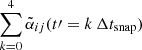
Finally, to compute all the dynamo coefficients simultaneously, we use the Iterative Removal of Sources (IROS) method (Hammersley et al. 1992). This algorithm has been developed for radio astronomy and applied to isolate contributions to the turbulent EMF from mean magnetic fields and currents (Dhang et al. 2024; Bendre et al. 2024). The key steps are:
-
Initialization: we start with zero values for αij and βij.
-
Fitting: at each spatial position, we fit the EMF time series against B and J to extract first-order estimates.
-
Refinement: we iteratively subtracted a percentage of the best-fit contributions from the EMF and updated the coefficients until convergence.
This method provides robust estimates, even in the presence of noise and permits the inclusion of priors, enhancing its applicability in high-resolution simulations of MRI-driven dynamos.
3. Results
In this paper, we focus on the dynamics of axisymmetric quantities, which correspond to y-averaged quantities in shearing boxes. Since shearing boxes are local models, we also averaged in the x-direction in order to filter some of the noise due to turbulence. In Paper I, we reported that the behavior of the solution could be divided into two regions in the vertical direction (i.e., perpendicular to the plane of the disk): a region closer to the midplane where the dynamics are governed by the MRI dynamo, and a region further away from the midplane dominated by magnetic buoyancy. We refer to these as the “MRI dynamo” zone and the “atmospheric zone”, respectively. In the following, these two zones will be defined as z ∈ [ − 2H, 2H] for the dynamo zone and z ∈ [ − 4H, −2H] and [2H, 4H] for the atmospheric zone.
3.1. Butterfly diagrams
We first show the butterfly diagrams (Figure 1) of the three important quantities to check whether the dynamo is indeed an αΩ dynamo:  ,
,  for the Ω effect and
  ,
,  for the α effect. The averaged magnetic field is around three times stronger at Pm = 90 than at Pm = 4. This value is expected since, in Paper I, the ratio of magnetic energy in the MRI dynamo zone is Emag, Pm = 90/Emag, Pm = 4 ≈ 7.8. The factor for the magnetic field between the two simulations is therefore ∼2.8. We note that this is slightly lower than what the magnetic energy scaling,
  , would predict because the plateau at high-Pm starts to set in. This shows that it is not only the turbulent field that is further amplified with Pm, but also the largest scale of the simulation, as was found by Guilet et al. (2022). In both simulations, the butterfly diagram of the averaged toroidal magnetic field,
  , shows some cycles. In the case of less turbulent Pm = 4 simulation, the cycles are very regular; whereas at Pm = 90, they are more chaotic and the period is harder to decipher. Furthermore,
  seems to be at larger scales for Pm = 4 than Pm = 90, while Paper I found the turbulence to be at larger scales for Pm = 90. This may seem contradictory at first, but it can be explained by the more intense turbulence at Pm = 90, as it is more efficient at generating (as can be seen by comparing the colorbars at Pm = 4 and Pm = 90 in Figure 1). Therefore, it is also more efficient at destroying the coherent magnetic fields,
  , and
, and  (as can be seen by the more turbulent cycles at Pm = 90).
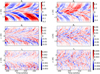 |
Fig. 1. Butterfly diagrams of the toroidal magnetic field (top), the radial magnetic field (middle), and the toroidal component of the EMF |

Once the coherent magnetic field reaches the atmosphere beyond |z|≥2H, the magnetic field behaves similarly and is as coherent, remaining on a similar scale for both Pm values. The result of the turbulence at larger scales is recovered for the other quantities, namely,  and
and  . Another difference that can be seen in the
  butterfly diagrams is the propagation velocity towards the atmosphere: at Pm = 4, the propagation is slower than at Pm = 90. However, once it is in the atmosphere, the magnetic field seems to propagate at very similar velocities in the two simulations. This seems to be coherent with the definition of the atmosphere, where dynamics are dominated by the buoyancy instabilities and the vertical mean flow (see Section 3.3), rather than by the MRI-driven dynamos, and, as was shown in Paper I, the buoyancy-driven region is less sensitive to Pm.
For the Pm = 4 simulation, the anti-correlations between  and
and  can be seen directly in the butterfly diagram. This correlation is harder to see at Pm = 90 as the radial magnetic field is more turbulent. Nevertheless, it is possible to see the correlation closer to the atmosphere, where the averaged magnetic field is less turbulent. The periodic cycle is also difficult to see in the
  diagram for the Pm = 90 case. For the EMF, the difference is striking between the two simulations: in the midplane, the y-component of the EMF is weaker than in the atmosphere for Pm = 4, while it is of similar amplitude for Pm = 90, which further shows the increased mean-field dynamo action with Pm. In addition, the cycle can clearly be seen for both simulations and they seem to be correlated with
  diagrams. The MRI-driven mean-field dynamo can be qualitatively interpreted as an αΩ dynamo.
Lastly, from these diagrams, we can estimate the simulation period by calculating time Fourier transforms of Bx at vertical positions z ∈ [ − 2H, 2H] and averaging the frequencies with the highest magnitude. We chose to use  as the α effect governs the generation of
  . The frequencies are shown in Table 1. The period is slightly shorter in the case of Pm = 90, which would be consistent with the stronger dynamo action. We note that, for a given simulation, there is some variability in the period between successive field reversals (as measured from the spacetime diagrams). However, all periods at Pm = 90 were systematically lower than at Pm = 4. Indeed, the period of an αΩ dynamo is given by Gressel & Pessah (2015) as
 (9)
(9)
Mean-field pattern periods for Pm = 4 and Pm = 90.
where kz is the vertical wavenumber estimated with  . To make a quantitative check whether it is correct, we need to compute the dynamo coefficients.
3.2. α effect and dynamo period
To confirm the effect of Pm on the αΩ dynamo, we computed the correlations to check whether the diagonal alpha effect is the dominant contribution to the toroidal  (Figure 2). We find that there is a strong correlation between
  and
and  for |z|≤2.5H, which decreases in the atmosphere. For |z|≥2.5H, the correlation between
  and
and  becomes sub-dominant compared to the correlation between
  and
and  . These results confirm that the dynamics of the atmosphere and the dynamo region of the shearing box are quite different. We also find that the correlation between the radial resistivity,
  , and the toroidal,
  , is not important in the dynamo region, which means that the turbulent resistivity can be neglected for the generation of the poloidal field from the toroidal field. In the correlations, the differences are quite small between Pm = 4 and Pm = 90. Due to the less turbulent dynamo, the correlations are slightly higher for Pm = 4, but they remain similar overall.
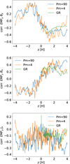 |
Fig. 2. Pearson correlations between |


The correlations hint that the dynamo cycle could be interpreted as an αΩ dynamo and that turbulent resistivity could be neglected to first-order for the EMF. To see whether we can recover the difference in the dynamo period between Pm = 4 and Pm = 90 in the dynamo coefficients, we compute the α dynamo coefficients with the IROS method, the correlation methods and the SVD method (Figure 3). With the IROS and correlation methods, the maximum value of the diagonal αyy effect is stronger by a factor ≈3 in the case of Pm = 90. The more chaotic aspect of the turbulence at Pm = 90 is also reflected in the larger amplitude fluctuations of the coefficient. In regions where the correlations are weaker, αyy computed using the correlation method is larger than the same quantity computed using the other methods. This is not surprising, since, when using the correlation method, the EMF is considered to be explained by only one dynamo coefficient at a time. The SVD method gives intermediate results between the IROS method and correlation methods. This corresponds to the atmosphere region for the diagonal αyy. For αyx, the main difference is close to the atmosphere boundaries, where SVD and IROS methods predict a stronger increase than the correlation method. Otherwise, all the methods roughly agree, except around |z|∼2H where αyx is slightly stronger with the correlation method.
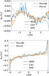 |
Fig. 3. α dynamo coefficients as a function of vertical coordinate, z. The solid, dashed, and dotted curves are calculated using the IROS, correlation (Corr), and SVD methods, respectively. Orange curves: Pm = 90. Blue curves: Pm = 4. |
Using the maximum value of αyy in the dynamo region, we compute the dynamo period using the theoretical formula from mean-field theory (Equation 9). The theoretical periods give a good agreement with what can be found in the butterfly diagrams as shown in Table 1. The difference in frequencies between above or below the midplane was not recovered for the Pm = 4 simulation. It might be due to the stochasticity of the turbulence over short timescales.
We also test whether these results hold when introducing a time-lag as Gressel & Pessah (2022) have identified a time-lag between the EMF and the mean magnetic field. In order to take into account this time-lag, the expression of the EMF becomes a convolution of the alpha tensor and the mean magnetic field
 (10)
(10)
This can be expressed in terms of frequencies in the Fourier space
 (11)
(11)
In Gressel & Pessah (2022), the frequency dependence was obtained using the “test-field” method. Because the dynamo coefficients are assumed to be independent of the mean magnetic field, this method computes the dynamo coefficients by evolving additional induction equations for a fluctuating magnetic field that are subject to prescribed, linearly independent, mean magnetic fields (known as “test fields”) and a velocity field taken directly from the simulations (Schrinner et al. 2005, 2007).
Because the test field method is computationally expensive and not implemented in PLUTO, we first calculated the correlations  between the EMF ℰy and the mean magnetic field, but replaced the instantaneous mean magnetic field
  (i.e., X or Y in Eq. 7) with the mean magnetic field at some time in the past
  , where t′=kΔtsnap is an integer multiple of the interval Δtsnap between successive snapshots. We found that the correlations decreased with t′, but they were still on the same order of magnitude when the time-lag was less than a fraction of the orbital time ∼0.3Ω−1 (notx shown). The correlation between ℰy and
  decreased faster than the correlation between ℰy and
  .
.
To test our results more precisely, we modified step 2 of the IROS algorithm, so that the fit of the EMF also included up to five previous snapshot time-intervals, Δtsnap (i.e., up to t′=0.5 orbits) of the mean magnetic field. In Figure 4, we compare the dynamo coefficients without taking into account the time-lag to the new instantaneous dynamo coefficients  ; i.e., with a time lag of t′=0) and to the sum of all contributions from the dynamo coefficient with time lags
  . The main difference is that the instantaneous diagonal dynamo coefficient
  is close to zero for |z|> 3H. Otherwise, the instantaneous coefficients are slightly smaller, but the values become similar when the contributions from previous snapshots are taken into account. Our results, therefore, remain robust when a time-lag is introduced in our statistical analysis. These results show that the large-scale dynamo can be interpreted as an αΩ dynamo and it gets stronger with increasing Pm.
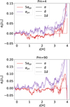 |
Fig. 4. Comparison of the effect of time-lags on the vertical profiles of α dynamo coefficients for Pm = 4 (top) and Pm = 90 (bottom). The purple curves correspond to the αyx component, and the red curves to αyy (compensated by a factor of five to make the coefficients easier to compare). Solid lines correspond to the coefficients α computed using the standard IROS method. dashed lines correspond to the instantaneous dynamo coefficients |

3.3. Off-diagonal α effect and propagation of the magnetic field
From these correlations, we can also see that the off-diagonal coefficient, αyx, is important in the atmosphere region (|z|> 2H). By using the value of the coefficient that is increasing away from the midplane (bottom panel of Figure 3), we can estimate the height at which the contribution of  to the EMF becomes more important than the diagonal coefficient,
  . This gives a result of |zoff − diag|≈2 − 2.5H, which corresponds roughly to the transition from the dynamo region to the atmosphere region. This explains why the dynamo period is well explained by its theoretical value depending only on αyy, even with the correlation between
  and
and  . To try to understand the physical impact of this off-diagonal coefficient, we computed the vertical turbulent pumping coefficient as
 (12)
(12)
In the closure relation of the EMF, the turbulent pumping γ is the antisymmetric component of the general α tensor and can therefore be written as
![Mathematical equation: $$ \begin{aligned} \overline{\mathcal{E} }= \boldsymbol{\gamma } \times \overline{B} + [\ldots ]. \end{aligned} $$](/articles/aa/full_html/2025/09/aa53714-25/aa53714-25-eq77.gif) (13)
(13)
Here, turbulent pumping can be interpreted as a velocity which acts on the mean magnetic field.
We compare the averaged vertical velocity  and γz in Figure 5. Once again, the difference between the dynamo region and the atmosphere region is striking. In the atmosphere region, the propagation of the magnetic field is dominated by the average velocity,
  , which is due to the stochastic effects of the kinetic pressure gradient as well as corresponding magnetic fluctuations and the magnetic buoyancy of the mean magnetic field (Suzuki & Inutsuka 2009). This explains why the vertical velocity is faster for Pm = 90. In the dynamo region, the vertical propagation is dominated by the turbulent pumping due to the small-scale turbulence. It is also stronger in the high-Pm case, which explains why the magnetic field in the butterfly diagram is moving faster towards the atmosphere. This shows the importance of the off-diagonal coefficient for the disk or neutron star dynamics, as a faster propagation of stronger magnetic fields towards the atmosphere could increase the efficiency of the disk or neutron star winds.
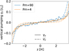 |
Fig. 5. Turbulent pumping coefficient, γz, calculated using the IROS method (solid lines), and averaged vertical velocity, |

3.4. Turbulent angular momentum transport
Another important impact of MRI turbulence on disks and stars is the transport of angular momentum. Paper I showed that the angular momentum transport, as parametrized by the ratio of volume-averaged turbulent stress to pressure, increases with Pm. In this paper, we would like to look at the region where angular momentum transport is the most important and distinguish the contribution due to the small-scale turbulence from that due to the mean-magnetic field. For this, we look at the Maxwell stress Mxy = −B′xB′y from the small-scales and from the largest scales  (Figure 6). The small-scale angular momentum transport is stronger close to the midplane (|z|< 2H) in both Pm regimes, while the large-scale angular momentum transport is more homogeneous in the whole simulation. In terms of amplitudes, the maximum value of the transport,
  , from the mean field is ≈4 lower than the one from the small scales, Mxy, and appears to be important mostly outside of the dynamo region (|z|> 2.5H). This is consistent with the spectral analysis carried out in Paper I, which showed that at z = 3.2H almost all the contribution to the power comes from kx = 0 and ky = 0. Since the transport from the mean-magnetic field amplitude happens via small patches, its integrated contribution for Pm = 4 and Pm = 90 contributes to 12%−16% of the total transport, respectively, which shows the importance of the mean-field dynamo for angular momentum transport as well.
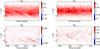 |
Fig. 6. Comparison of the butterfly diagrams of the Maxwell stress, Mxy, due to the small-scale magnetic field component (top) and the large-scale (mean) magnetic field component (bottom) for magnetic Prandtl number Pm = 4 (left) and Pm = 90 (right). Note that, in general, the mean magnetic field (bottom) is smaller than Mxy (top) by about a factor of four. |
4. Comparison with a 3D GRMHD simulation
In this section, we compare the properties of the MRI dynamo in the shearing box simulations to the results of a 3D ideal GRMHD simulation in which the remnant massive neutron star was long-lived (Kiuchi et al. 2024). The GRMHD simulation employed equatorial symmetry. In the GRMHD simulation, we found evidence for an αΩ dynamo in the remnant neutron star, which generated a cyclical mean magnetic field eventually leading to the launch of a jet. In order to compare the two simulations (local and global), we take azimuthally averaged data from the global simulation at a cylindrical radius of s0 = 28.5 km and estimate an “equivalent” scale-height, HGRMHD = 7 km1. Thus, in both configurations, the vertical density profile roughly drops by one order of magnitude at the same vertical height. We note that the scale height as defined in disks,  , where cs is the sound speed, would give a different value (H ≈ 15 km) in the neutron star remnant. The shear is also slightly sub-Keplerian (q = 1.34) in the GRMHD simulation.
With this value, we compared the correlations above the midplane (Figure 2) at s0 = 28.5 km and found a good agreement between the shearing box simulations (blue and orange curves) and the GRMHD simulations (green curve). It seems that the global simulation correlations are lower. This is most likely due to a more turbulent and/or chaotic dynamo in global simulations or it could be due to GR effects as lower correlations have been found in different GR simulations (Jacquemin-Ide et al. 2024).
To obtain a more quantitative comparison for the dynamo, we use the value of the sound speed averaged between z ∈ [0, 10] km in the binary neutron star simulation to scale the maximum value of the diagonal αyy in shearing box simulations (Figure 7). The mean-field dynamo in the global simulation has a slightly lower α effect than the Pm = 4 shearing box simulation, but much lower than the Pm = 90. Since we would expect a lower α-effect for a shearing box with Pm = 1, this shows that the global simulation, which has a numerical Prandtl number of order unity, PmGRMHD ≈ O(1), has a slightly more efficient αΩ dynamo than the shearing box dynamo. We also find that the mean-field dynamo in the GRMHD simulations is less efficient at smaller radii, where the fluid is denser.
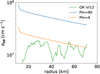 |
Fig. 7. Comparison of the maximum value of the diagonal αϕϕ computed using the IROS method from shearing box simulations at different magnetic Prandtl numbers of Pm = 4 and 90 (orange and blue curves, respectively) as well as from the GRMHD simulation (green curve). The sound speed of the GRMHD simulation was used to scale the shearing box simulation results. |
This could be attributed to several different explanations. First, it is most likely an impact of the shear rate. In the hypermassive neutron star remnant, the angular frequency first increases with radius (MRI-stable region) and peaks at ∼10 km, after which it decreases with radius (MRI-unstable region). Thus, the shear rate (q ≡ dlnΩ/dlnr) decreases with decreasing radius in the MRI-unstable region and reaches q = 0 at ∼10 km, which leads to reduced turbulence and dynamo efficiency. Finally, GR effects become non-negligible in the core region and might play a role in the decrease in the dynamo efficiency at small radii. In any case, the comparison shows that if the GRMHD simulation was in the right regime of magnetic Prandtl number of Pm ∼ 1010 − 14 (Guilet et al. 2017), the dynamo period and the mean-field growth rate are expected to be 60% faster, which would lead to a faster launch of a jet. In addition, the mean magnetic field should also be further amplified by a factor of ≈1000.744/2 = 5.5. This could have important astrophysical consequences, as the Poynting-flux luminosity and the magnetization parameter of the jet could become stronger by a factor of ∼30.
5. Discussion
5.1. Disk versus neutron star differences
The shearing box simulations used in this paper were set up to model MRI turbulence in a disk. However, there are some differences between disks and neutron stars (i.e., protoneutron stars in core-collapse supernovae and hypermassive neutron stars in binary neutron star mergers) that could impact the results. The first one is the spherical and cylindrical geometry of PNS and HMNS, respectively, compared to the cylindrical geometry of disks. This was studied by Reboul-Salze et al. (2021), who showed that similar results between shearing box and global simulations of PNS could be obtained in shearing boxes with an azimuthal length, Ly ∼ r, where the curvature of the star can be neglected. The shearing box simulations in the current paper are characterized by Ly = 4H; therefore, they match the curvature of a neutron star remnant at a radius of r = 4HGRMHD ≈ 28 km.
Another difference is that the shearing box neglects the stratification in the radial direction, which global models take into account. For the radial box size, we employed Lx = 4H, this would correspond to Lx = 4HGRMHD ≈ 28 km. In protoneutron stars (or hypermassive neutron stars), the density would change over this radial length scale. On the other hand, our relatively large shearing box size allows for a larger domain for the computation of averages in the radial direction, which may explain why the correlations are higher than in the global GRMHD simulations.
Lastly, the force balance (between gravity and centrifugal forces) may be different in protoneutron stars or hypermassive neutron stars compared to that in an accretion disk. This could lead to a lower shear rate than q = 1.5, thereby changing the scaling of the magnetic field with Pm (cf. Held & Mamatsashvili 2022, Figure 12). However, this change in the scaling was found for vertically unstratified boxes with a large aspect ratio. With this configuration, the winding of a strong toroidal field, which highly depends on the shear rates, causes most of the dynamics to remain at large scales and depend less on small scales (i.e., Pm). The dependence of the Pm scaling on the shear rate might change with cubic boxes or with vertical stratification, which introduces different scales. However, this aspect is left to future studies.
5.2. Impact of thermal stratification
The shearing box simulations here are isothermal. Depending on the heating and cooling timescales, this is a good approximation. For protoneutron stars or hypermassive neutron stars, the neutrino cooling timescale is of the order O(1−10)s and thus longer than the dynamo timescale  in fast rotating cases. For these objects, adding thermal stratification could slightly change the results. However, the thermal diffusion due to neutrinos is higher than the viscosity,
 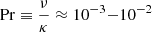 (Reboul-Salze et al. 2022), which should limit the changes. In the case of disks, future work should also take into account the effects of neutrino cooling, thermodynamics, and temperature and density-dependent diffusion coefficients, to probe their thermal stability in the large-Pm regime.
6. Conclusions
We carried out a new analysis of the shearing box simulations presented in Paper I to investigate the impact of the magnetic Prandtl number, Pm, on the MRI-driven mean-field dynamo. We studied the mean-field dynamo in the regime of high-magnetic Prandtl number, the ratio of viscosity over resistivity, which is relevant for binary neutron star or black hole-neutron star mergers, protoneutron stars, and the inner regions of active galactic nuclei (AGNs) and X-ray binary disks.
Our main finding is that the mean magnetic field follows the scaling law derived for the magnetic energy in Held et al. (2024). We showed that the mean-magnetic field evolution can be described by an αΩ dynamo, even in the high-Pm regime. We also computed the dynamo coefficients, which also increase with Pm, but with a smaller factor than for the magnetic field. We also found that the dynamo period is also shortened at high Pm and we have a good agreement between the theoretical estimation of the dynamo period and the butterfly diagrams.
We also deduced a range of different behaviors for the mean-field dynamo depending on the vertical height. In the atmosphere, the off-diagonal coefficient, αϕs, dominates the contribution to the electromotive force that generates the poloidal magnetic field. While it does not dominate closer to the mid-plane of the disk, this coefficient impacts the propagation of the magnetic field as the turbulent pumping derived from it leads to a faster vertical propagation than the mean vertical velocity. The propagation speed increases with Pm, which can be explained by an increase in the off-diagonal dynamo coefficients. Overall, we recover the differences between the MRI-driven dynamo and magnetic buoyancy instabilities found in Paper I.
For systems in the high-Pm regime, the amplification of large-scale magnetic fields happening in ideal MHD, with a numerical magnetic Prandtl number of order of 1, is expected to be realistically further amplified by at least a factor of 5. This increased efficiency of the MRI-driven dynamo could have many important physical consequences: the jet found in GRMHD simulations of binary neutron star mergers could be launched earlier and be more luminous and more relativistic. In black hole disk simulations, the magnetically arrested disk state (Tchekhovskoy et al. 2011) could be reached faster, which would facilitate the launch of a relativistic jet. In the context of core-collapse supernovae, the impact of the increased efficiency would be similar: this would more easily lead to greater Lorentz factors in relativistic jets and greater luminosity from the magnetic spin-down of the protoneutron star.
To study the impact of these enhanced large-scale magnetic fields in global simulations where the high-Pm regime is numerically not reachable, MRI turbulence has to be included using subgrid models. Often, only the angular momentum transport is included using viscous hydrodynamics (alpha-disk models) (Fernández & Metzger 2013; Fujibayashi et al. 2018, 2020a,b; Just et al. 2023). This neglects the other impacts of the mean magnetic field, such as the disk winds, further extraction of rotational energy to power a jet, and other effects. Some models use a scalar diagonal dynamo coefficient in the mean-field formulation to have the amplification and the dynamo cycle (Del Zanna et al. 2022), but the dynamo coefficients or the saturated magnetic energy are often lower than what is found in this paper (Shibata et al. 2021; Most 2023). Moreover, the astrophysical consequences of adding off-diagonal dynamo coefficients remain unknown. However, it could make 2D axisymmetric global simulations more realistic in future investigations of the parameter space of binary neutron star mergers.
This is the density scale-height, which we measured directly from the global simulation.
Acknowledgments
Simulations were run on the Sakura, Cobra, and Raven clusters at the Max Planck Computing and Data Facility (MPCDF) in Garching, Germany. This work was in part supported by the Grant-in-Aid for Scientific Research (grant Nos. 23H04900, 23H01172, 23K25869) of Japan MEXT/JSPS.
References
- Abbott, B. P., Abbott, R., Abbott, T. D., et al. 2017a, ApJ, 848, L13 [CrossRef] [Google Scholar]
- Abbott, B. P., Abbott, R., Abbott, T. D., et al. 2017b, ApJ, 848, L12 [Google Scholar]
- Aguilera-Miret, R., Palenzuela, C., Carrasco, F., Rosswog, S., & Viganò, D. 2024, Phys. Rev. D, 110, 083014 [Google Scholar]
- Aloy, M. Á., & Obergaulinger, M. 2021, MNRAS, 500, 4365 [Google Scholar]
- Balbus, S. A., & Henri, P. 2008, ApJ, 674, 408 [NASA ADS] [CrossRef] [Google Scholar]
- Bendre, A. B., Schober, J., Dhang, P., & Subramanian, K. 2024, MNRAS, 530, 3964 [Google Scholar]
- Brandenburg, A. 2018, J. Plasma Phys., 84, 735840404 [Google Scholar]
- Brandenburg, A., Nordlund, A., Stein, R. F., & Torkelsson, U. 1995, ApJ, 446, 741 [NASA ADS] [CrossRef] [Google Scholar]
- Bucciantini, N., Metzger, B. D., Thompson, T. A., & Quataert, E. 2012, MNRAS, 419, 1537 [NASA ADS] [CrossRef] [Google Scholar]
- Bugli, M., Guilet, J., Obergaulinger, M., Cerdá-Durán, P., & Aloy, M. A. 2020, MNRAS, 492, 58 [NASA ADS] [CrossRef] [Google Scholar]
- Christie, I. M., Lalakos, A., Tchekhovskoy, A., et al. 2019, MNRAS, 490, 4811 [NASA ADS] [CrossRef] [Google Scholar]
- Combi, L., & Siegel, D. M. 2023, Phys. Rev. Lett., 131, 231402 [Google Scholar]
- Davis, S. W., Stone, J. M., & Pessah, M. E. 2010, ApJ, 713, 52 [NASA ADS] [CrossRef] [Google Scholar]
- Del Zanna, L., Tomei, N., Franceschetti, K., Bugli, M., & Bucciantini, N. 2022, Fluidika, 7, 87 [NASA ADS] [Google Scholar]
- Dhang, P., Bendre, A. B., & Subramanian, K. 2024, MNRAS, 530, 2778 [Google Scholar]
- Drout, M. R., Soderberg, A. M., Gal-Yam, A., et al. 2011, ApJ, 741, 97 [NASA ADS] [CrossRef] [Google Scholar]
- Duncan, R. C., & Thompson, C. 1992, ApJ, 392, L9 [Google Scholar]
- Fernández, R., & Metzger, B. D. 2013, MNRAS, 435, 502 [CrossRef] [Google Scholar]
- Fernández, R., Tchekhovskoy, A., Quataert, E., Foucart, F., & Kasen, D. 2019, MNRAS, 482, 3373 [CrossRef] [Google Scholar]
- Fromang, S., Papaloizou, J., Lesur, G., & Heinemann, T. 2007, A&A, 476, 1123 [NASA ADS] [CrossRef] [EDP Sciences] [Google Scholar]
- Fujibayashi, S., Kiuchi, K., Nishimura, N., Sekiguchi, Y., & Shibata, M. 2018, ApJ, 860, 64 [NASA ADS] [CrossRef] [Google Scholar]
- Fujibayashi, S., Wanajo, S., Kiuchi, K., et al. 2020a, ApJ, 901, 122 [NASA ADS] [CrossRef] [Google Scholar]
- Fujibayashi, S., Shibata, M., Wanajo, S., et al. 2020b, Phys. Rev. D, 102, 123014 [Google Scholar]
- Fujibayashi, S., Sekiguchi, Y., Shibata, M., & Wanajo, S. 2023, ApJ, 956, 100 [Google Scholar]
- Gao, H., Ding, X., Wu, X.-F., Zhang, B., & Dai, Z.-G. 2013, ApJ, 771, 86 [Google Scholar]
- Giacomazzo, B., & Perna, R. 2013, ApJ, 771, L26 [NASA ADS] [CrossRef] [Google Scholar]
- Goldstein, A., Veres, P., Burns, E., et al. 2017, ApJ, 848, L14 [CrossRef] [Google Scholar]
- Gompertz, B. P., O’Brien, P. T., & Wynn, G. A. 2014, MNRAS, 438, 240 [NASA ADS] [CrossRef] [Google Scholar]
- Gottlieb, O., Moseley, S., Ramirez-Aguilar, T., et al. 2022a, ApJ, 933, L2 [NASA ADS] [CrossRef] [Google Scholar]
- Gottlieb, O., Lalakos, A., Bromberg, O., Liska, M., & Tchekhovskoy, A. 2022b, MNRAS, 510, 4962 [CrossRef] [Google Scholar]
- Gottlieb, O., Issa, D., Jacquemin-Ide, J., et al. 2023a, ApJ, 954, L21 [Google Scholar]
- Gottlieb, O., Metzger, B. D., Quataert, E., et al. 2023b, ApJ, 958, L33 [NASA ADS] [CrossRef] [Google Scholar]
- Gressel, O., & Pessah, M. E. 2015, ApJ, 810, 59 [NASA ADS] [CrossRef] [Google Scholar]
- Gressel, O., & Pessah, M. E. 2022, ApJ, 928, 118 [Google Scholar]
- Guilet, J., Müller, E., & Janka, H.-T. 2015, MNRAS, 447, 3992 [NASA ADS] [CrossRef] [Google Scholar]
- Guilet, J., Bauswein, A., Just, O., & Janka, H.-T. 2017, MNRAS, 471, 1879 [NASA ADS] [CrossRef] [Google Scholar]
- Guilet, J., Reboul-Salze, A., Raynaud, R., Bugli, M., & Gallet, B. 2022, MNRAS, 516, 4346 [NASA ADS] [CrossRef] [Google Scholar]
- Hammersley, A., Ponman, T., & Skinner, G. 1992, Nucl. Instrum. Meth. Phys. Res. A, 311, 585 [Google Scholar]
- Hawley, J. F., Gammie, C. F., & Balbus, S. A. 1996, ApJ, 464, 690 [NASA ADS] [CrossRef] [Google Scholar]
- Hayashi, K., Kiuchi, K., Kyutoku, K., Sekiguchi, Y., & Shibata, M. 2025, Phys. Rev. Lett., 134, 211407 [Google Scholar]
- Held, L. E., & Mamatsashvili, G. 2022, MNRAS, 517, 2309 [NASA ADS] [Google Scholar]
- Held, L. E., Mamatsashvili, G., & Pessah, M. E. 2024, MNRAS, 530, 2232 [NASA ADS] [CrossRef] [Google Scholar]
- Jacquemin-Ide, J., Rincon, F., Tchekhovskoy, A., & Liska, M. 2024, MNRAS, 532, 1522 [Google Scholar]
- Janiuk, A., & Yuan, Y. F. 2010, A&A, 509, A55 [NASA ADS] [CrossRef] [EDP Sciences] [Google Scholar]
- Just, O., Vijayan, V., Xiong, Z., et al. 2023, ApJ, 951, L12 [NASA ADS] [CrossRef] [Google Scholar]
- Kiuchi, K., Reboul-Salze, A., Shibata, M., & Sekiguchi, Y. 2024, Nat. Astron., 8, 298 [Google Scholar]
- Komissarov, S. S., & Barkov, M. V. 2009, MNRAS, 397, 1153 [NASA ADS] [CrossRef] [Google Scholar]
- Krause, F., & Raedler, K. H. 1980, Mean-field Magnetohydrodynamics and Dynamo Theory (Oxford: Pergamon Press) [Google Scholar]
- Kuroda, T., Arcones, A., Takiwaki, T., & Kotake, K. 2020, ApJ, 896, 102 [NASA ADS] [CrossRef] [Google Scholar]
- Mamatsashvili, G., Chagelishvili, G., Pessah, M. E., Stefani, F., & Bodo, G. 2020, ApJ, 904, 47 [NASA ADS] [CrossRef] [Google Scholar]
- Margalit, B., Metzger, B. D., Thompson, T. A., Nicholl, M., & Sukhbold, T. 2018, MNRAS, 475, 2659 [NASA ADS] [CrossRef] [Google Scholar]
- Metzger, B. D., & Piro, A. L. 2014, MNRAS, 439, 3916 [NASA ADS] [CrossRef] [Google Scholar]
- Metzger, B. D., Quataert, E., & Thompson, T. A. 2008, MNRAS, 385, 1455 [CrossRef] [Google Scholar]
- Metzger, B. D., Giannios, D., Thompson, T. A., Bucciantini, N., & Quataert, E. 2011, MNRAS, 413, 2031 [Google Scholar]
- Metzger, B. D., Beniamini, P., & Giannios, D. 2018, ApJ, 857, 95 [NASA ADS] [CrossRef] [Google Scholar]
- Moffatt, H. K. 1978, Cambridge Monographs on Mechanics and Applied Mathematics (Cambridge: Cambridge University Press) [Google Scholar]
- Moiseenko, S. G., Bisnovatyi-Kogan, G. S., & Ardeljan, N. V. 2006, MNRAS, 370, 501 [NASA ADS] [CrossRef] [Google Scholar]
- Mooley, K. P., Deller, A. T., Gottlieb, O., et al. 2018, Nature, 561, 355 [Google Scholar]
- Most, E. R. 2023, Phys. Rev. D, 108, 123012 [Google Scholar]
- Mösta, P., Richers, S., Ott, C. D., et al. 2014, ApJ, 785, L29 [CrossRef] [Google Scholar]
- Mösta, P., Radice, D., Haas, R., Schnetter, E., & Bernuzzi, S. 2020, ApJ, 901, L37 [CrossRef] [Google Scholar]
- Musolino, C., Rezzolla, L., & Most, E. R. 2025, ApJ, 984, L61 [Google Scholar]
- Nicholl, M., Smartt, S. J., Jerkstrand, A., et al. 2013, Nature, 502, 346 [NASA ADS] [CrossRef] [Google Scholar]
- Obergaulinger, M., Just, O., & Aloy, M. A. 2018, J. Phys. G Nucl. Part. Phys., 45, 084001 [NASA ADS] [CrossRef] [Google Scholar]
- Pessah, M. E., Chan, C.-K., & Psaltis, D. 2007, ApJ, 668, L51 [Google Scholar]
- Racine, É., Charbonneau, P., Ghizaru, M., Bouchat, A., & Smolarkiewicz, P. K. 2011, ApJ, 735, 46 [Google Scholar]
- Reboul-Salze, A., Guilet, J., Raynaud, R., & Bugli, M. 2021, A&A, 645, A109 [NASA ADS] [CrossRef] [EDP Sciences] [Google Scholar]
- Reboul-Salze, A., Guilet, J., Raynaud, R., & Bugli, M. 2022, A&A, 667, A94 [NASA ADS] [CrossRef] [EDP Sciences] [Google Scholar]
- Rempel, E. L., Lesur, G., & Proctor, M. R. E. 2010, Phys. Rev. Lett., 105, 044501 [Google Scholar]
- Rincon, F. 2019, J. Plasma Phys., 85, 205850401 [NASA ADS] [CrossRef] [Google Scholar]
- Riols, A., Rincon, F., Cossu, C., et al. 2015, A&A, 575, A14 [NASA ADS] [CrossRef] [EDP Sciences] [Google Scholar]
- Riols, A., Rincon, F., Cossu, C., et al. 2017, A&A, 598, A87 [NASA ADS] [CrossRef] [EDP Sciences] [Google Scholar]
- Rossi, E. M., Armitage, P. J., & Menou, K. 2008, MNRAS, 391, 922 [Google Scholar]
- Sarin, N., Omand, C. M. B., Margalit, B., & Jones, D. I. 2022, MNRAS, 516, 4949 [Google Scholar]
- Savchenko, V., Ferrigno, C., Kuulkers, E., et al. 2017, ApJ, 848, L15 [NASA ADS] [CrossRef] [Google Scholar]
- Schrinner, M., Rädler, K. H., Schmitt, D., Rheinhardt, M., & Christensen, U. 2005, Astron. Nachr., 326, 245 [Google Scholar]
- Schrinner, M., Rädler, K.-H., Schmitt, D., Rheinhardt, M., & Christensen, U. R. 2007, Geophys. Astrophys. Fluid Dyn., 101, 81 [Google Scholar]
- Shi, J., Krolik, J. H., & Hirose, S. 2010, ApJ, 708, 1716 [NASA ADS] [CrossRef] [Google Scholar]
- Shi, J.-M., Stone, J. M., & Huang, C. X. 2016, MNRAS, 456, 2273 [NASA ADS] [CrossRef] [Google Scholar]
- Shibata, M., Fujibayashi, S., & Sekiguchi, Y. 2021, Phys. Rev. D, 104, 063026 [NASA ADS] [CrossRef] [Google Scholar]
- Suzuki, T. K., & Inutsuka, S.-I. 2009, ApJ, 691, L49 [Google Scholar]
- Tchekhovskoy, A., Narayan, R., & McKinney, J. C. 2011, MNRAS, 418, L79 [NASA ADS] [CrossRef] [Google Scholar]
- Winteler, C., Käppeli, R., Perego, A., et al. 2012, ApJ, 750, L22 [Google Scholar]
- Woosley, S. E. 1993, ApJ, 405, 273 [Google Scholar]
All Tables
All Figures
|
Fig. 1. Butterfly diagrams of the toroidal magnetic field (top), the radial magnetic field (middle), and the toroidal component of the EMF |
| In the text | |
|
Fig. 2. Pearson correlations between |
| In the text | |
|
Fig. 3. α dynamo coefficients as a function of vertical coordinate, z. The solid, dashed, and dotted curves are calculated using the IROS, correlation (Corr), and SVD methods, respectively. Orange curves: Pm = 90. Blue curves: Pm = 4. |
| In the text | |
|
Fig. 4. Comparison of the effect of time-lags on the vertical profiles of α dynamo coefficients for Pm = 4 (top) and Pm = 90 (bottom). The purple curves correspond to the αyx component, and the red curves to αyy (compensated by a factor of five to make the coefficients easier to compare). Solid lines correspond to the coefficients α computed using the standard IROS method. dashed lines correspond to the instantaneous dynamo coefficients |
| In the text | |
|
Fig. 5. Turbulent pumping coefficient, γz, calculated using the IROS method (solid lines), and averaged vertical velocity, |
| In the text | |
|
Fig. 6. Comparison of the butterfly diagrams of the Maxwell stress, Mxy, due to the small-scale magnetic field component (top) and the large-scale (mean) magnetic field component (bottom) for magnetic Prandtl number Pm = 4 (left) and Pm = 90 (right). Note that, in general, the mean magnetic field (bottom) is smaller than Mxy (top) by about a factor of four. |
| In the text | |
|
Fig. 7. Comparison of the maximum value of the diagonal αϕϕ computed using the IROS method from shearing box simulations at different magnetic Prandtl numbers of Pm = 4 and 90 (orange and blue curves, respectively) as well as from the GRMHD simulation (green curve). The sound speed of the GRMHD simulation was used to scale the shearing box simulation results. |
| In the text | |
Current usage metrics show cumulative count of Article Views (full-text article views including HTML views, PDF and ePub downloads, according to the available data) and Abstracts Views on Vision4Press platform.
Data correspond to usage on the plateform after 2015. The current usage metrics is available 48-96 hours after online publication and is updated daily on week days.
Initial download of the metrics may take a while.