© The Authors 2025

1 Introduction

Phase curves of small bodies are valuable tools for computing absolute magnitudes and, through suitable photometric models, phase coefficients that may be related to surface properties. In a nutshell, the phase curve of a small body shows the change in apparent magnitude (normalized to the distances object-Sun, r, and object-observer, Δ) with phase angle (α). The phase angle is related to the fraction of illuminated surface seen by the observer.

Absolute magnitudes (H) are related to the diameter and albedo of the small body (Bowell & Lumme 1979). They aim to quantify the amount of light scattered by the object in contrast to the amount of light it emits, which occurs in thermal infrared wavelengths. On the other hand, the phase coefficients depend on the chosen photometric model. A variety of such models exist, but for the sake of simplicity, and because our input data is relatively sparse (see Sect. 2), we use models with few parameters (Sect. 3); namely, the ${\mathrm{H}\mathrm{G}}_{12}^{\ast }$ (Penttilä et al. 2016) and a linear model, both of which have only two free parameters. The first model is an adaptation of the HG₁G₂ (Muinonen et al. 2010) that is better suited for working with sparse data, while the second is the more straightforward form that a phase curve could adopt.

Phase curves have been studied mainly in the visible range (500–900 nm), first using traditional observing campaigns (for instance, Belskaya & Shevchenko 2000; Shevchenko et al. 2016) and more recently using large photometric surveys or massive databases (for example, Oszkiewicz et al. 2011; Vereš et al. 2015; Colazo et al. 2021, among others). These works used photometric measurements in a single filter, often Johnson’s V, and thus missed the nuances of how the spectra, or photo-spectra, behave with changing phase angles. A typical phase curve shows a linear behavior for α > 7–10 deg. Some objects also show an increase in brightness at low α, especially below five degrees, called the opposition effect (OE), which may be due to a decrease in the interparticle shadows (Hapke 1963), coherent backscattering (Muinonen 1989), or a combination of both.

The logical extension of single-wavelength studies is the use of multiwavelength data, which allows us to mimic the reflectance spectra of small bodies. Among the first systematic studies are the works by Mahlke et al. (2021), Alvarez-Candal et al. (2022a), and Alvarez-Candal (2024b), which performed analyses of multiwavelength phase curves, demonstrating their importance. For their most interesting results, we can mention the apparent changes in the phase coefficients with wavelength (Mahlke et al. 2021; Carry et al. 2024), which should be interpreted with great care (Alvarez-Candal 2024a), or the changes in spectral slope with α, which show that some objects may suffer bluing and reddening in different phase angle intervals (Wilawer et al. 2024; Alvarez-Candal 2024b; Colazo et al. 2025).

Unfortunately, to our knowledge, no systematic effort has been made to study the phase curves of small bodies in near-infrared (NIR) wavelengths, possibly because the curves are not expected to show a strong OE (Sanchez et al. 2012) and because NIR observations are more challenging than in the visible, particularly when moving to the redder part of the spectrum (H and K regions), where the brightness of the sky may outshine the small bodies, making their detection difficult.

The objectives of this work are: first, to produce a database of absolute magnitudes in the NIR combining data from different photometric catalogs (see Sect. 2); second, to better understand which photometric model will be more beneficial to analyze NIR phase curves; and third, to check the impact of having phase curves on limited α coverage, in particular when low phase angle data is not available. We use data from four catalogs that provide NIR magnitudes, including the Y, J, H, and K filters. We have organized this work such that in the next section we describe the four databases used and the transformations from one to the other. In Section 3, we describe the data processing. The last two sections are devoted to presenting and discussing the results.

2 Data

As was mentioned above, we utilized four catalogs of NIR magnitudes that cover the YJHK region (≈1000–2400 nm). Each catalog was obtained at different facilities, so the photometric systems are not identical. Therefore, we used suitable transformations found in the literature to minimize their systematic differences. We have aimed to transform all surveys to the MOVIS system because it is the only one that covers all four filters. In this work, we use the terms “filter” and “magnitude” interchangeably, as there should be no confusion for the reader.

The following subsections describe the catalogs used and the corresponding transformations (also summarized in Appendix A). The total number of input objects can be seen in Table 1. The transmission curves of all filters can be seen in Fig. 1.

2.1 MOVIS

The Moving Objects from VISTA survey (MOVIS, Popescu et al. 2016) extracts the small body data from the VISTA Hemisphere Survey (VHS) carried out at the ESO-VISTA 4-m telescope in Cerro Paranal, Antofagasta, Chile. MOVIS collects data in the Y_M, J_M, H_M, and K_M filters of 58 502 objects (MOVIS-M catalog) with 73 029 lines in total. The filter-by-filter breakdown is shown in Table 1. All details of matching the small bodies to the VISTA-VHS survey data can be found in Popescu et al. (2016). We use this catalog as the reference because it includes data in all four filters. The data are available at the Centre de Données de Strasbourg¹.

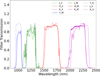Fig. 1 Transmission curves of all filters in the NIR used in this work. Different colors label different filters, and different line styles indicate different instruments. The different labels are 2 for 2MASS, M for MOVIS, D for DES, and U for UHS.

2.2 2MASS

The 2 Microns All Sky Survey (2MASS, Skrutskie et al. 2006) observed almost the whole sky in three photometric filters, J₂, H₂, and K₂, using two 1.3 m telescopes, one in Mount Hopkins, Arizona, USA, and one in Cerro Tololo, Coquimbo region, Chile. Among the almost 5 × 10⁸ point-like sources cataloged, the survey detected several thousand small bodies (see Sykes et al. 2000, for details). The catalog is available in the Small Body Node of the Planetary Data System (Sykes et al. 2020).

To transform the magnitudes from the 2MASS system to the MOVIS system, we used the equations in Popescu et al. (2016), which we repeat here (note that we use the subindexes M and 2 for the MOVIS and 2MASS, respectively. We keep this notation, which should be transparent to the reader, when necessary): $$\begin{array}{rl}& J_M=J_2-0.077(J-H{)}_2,\\ & H_M=H_2+0.032(J-H{)}_2,\text{\hspace{0.17em}and\hspace{0.17em}}\\ & K_M=K_2+0.010(J-K{)}_2.\end{array}$$(1)

The transformations shown in Eq. (1) depend on the color of the object, which we do not know a priori. Moreover, not all objects were observed in all filters, or simultaneously. Therefore, we decided to use solar colors in all cases (we used the same criterion in all transformations below). Suitable solar colors were chosen from the literature in the respective photometric system. In the case of 2MASS, we used the solar colors in Casagrande et al. (2012): (J − H)₂ = 0.286 and (J − K)₂ = 0.362. The offsets are J_M − J₂ ≈ −0.02, H_M − H₂ ≈ 0.01, and K_M − K₂ ≈ 0.004. The input 2MASS catalog contains 38 280 lines² for 19 394 objects.

2.3 UHS

The UKIRT Hemisphere Survey (UHS) currently observes the northern sky with three photometric filters: J_U, H_U, and K_U, although its current data release only includes J_U and K_U data. Within the survey, Morrison et al. (2024) extracted the data of small bodies serendipitously observed. The final catalog contains 15 233 lines for 13 662 objects.

The UHS magnitudes were transformed into the MOVIS system using two steps. The first one, from Hodgkin et al. (2009), transforms the magnitudes from UKIRT to 2MASS: $$\begin{array}{rl}& J_2=J_U+0.065(J-H{)}_U,\\ & H_2=H_U+0.030-0.070(J-H{)}_U,\text{\hspace{0.17em}and\hspace{0.17em}}\\ & K_2=K_U-0.010(J-K{)}_U,\end{array}$$(2)

where we used the solar colors from Willmer (2018): (J − H)_U = 0.35 and (J − K)_U = 0.40. The offsets are J₂ − J_U ≈ 0.02, H₂ − H_U ≈ 0.05, and K₂ − K_U ≈ 0.004. Then, we applied the 2MASS → MOVIS transformation from Eq. (1). The data are available as a machine-readable file online³.

2.4 DES

The Dark Energy Survey (DES, Dark Energy Survey Collaboration 2016) utilizes the DECAM camera and a set of filters spanning the visible spectrum (not used in this work) and the Y_D filter. DES observed 5 000 square degrees of the southern sky using the 4-m Blanco Telescope in Cerro Tololo Observatory, Chile. Although its primary purpose is cosmological, thousands of small bodies were serendipitously observed (e.g., Bernardinelli et al. 2022; Carruba et al. 2024). The Y_D filter catalog contains 135 092 lines for 95 802 objects⁴.

The DES survey was carried out using the AB photometric system, while the others used here are in the Vega system. This difference in reference systems introduces an offset in the zero points, which should be accounted for, especially when dealing with colors. We applied the transformation $$Y_M=Y_D-0.6,$$(3)

from González-Fernández et al. (2017). The DES data are available online⁵. Joining all four catalogs, we end up with an input of 261 634 lines for 169 256 objects.

3 Data processing

The data were processed following the same structure as in our previous works (Alvarez-Candal et al. 2022a; Alvarez-Candal 2024b), with adaptations to work with NIR data (for example, the transformation between the different photometric systems mentioned above). As in the cited works, the processing first creates or opens, if it exists, the probability distribution of rotational amplitudes, P_A(Δm), for each small body, A, and then uses it, convolved with the observational errors, to randomly extract 10 000 points to fit the selected photometric model. The final products are the probability distributions, P_A(H, Coeffs), of each small body’s absolute magnitude and phase coefficients. This processing primarily affects the uncertainty estimates, not the central values.

In this work, we use two photometric models. First, the ${\mathrm{H}\mathrm{G}}_{12}^{\ast }$ model (Penttilä et al. 2016) and then a linear model where M(α) = H + βα. The ${\mathrm{H}\mathrm{G}}_{12}^{\ast }$ model is an adaptation of the IAU adopted HG₁G₂ model described by $$M(\alpha )=H-2.5\log [G_1{\mathrm{\Phi }}_1(\alpha )+G_2{\mathrm{\Phi }}_2(\alpha )+(1-G_1-G_2){\mathrm{\Phi }}_3(\alpha )],$$(4)

where M(α) = m − 5 log (RΔ) is the reduced magnitude, m is the apparent magnitude, R(Δ) is the helio(topo)centric distance in astronomical units, H is the absolute magnitude, Φ_i are known functions of α, and G_i are the phase coefficients. In the ${\mathrm{H}\mathrm{G}}_{12}^{\ast }$ model, G₁ and G₂ are parametrized by $G_{12}^{\ast }$ according to G₁ = 0.84293649 × $G_{12}^{\ast }$ and G₂ = 0.53513350 × (1 − $G_{12}^{\ast }$). We ran three experiments: i) fitting the ${\mathrm{H}\mathrm{G}}_{12}^{\ast }$ model, ii) fitting the linear model, and iii) fitting the linear model but including only α > 9.5 deg to accomplish the objectives mentioned in the introduction.

The first exercise involved studying how well the ${\mathrm{H}\mathrm{G}}_{12}^{\ast }$ model, which is nonlinear, fits the phase curves in the NIR, especially remembering that they may not show a strong nonlinear behavior (see Sanchez et al. 2012), i.e., they may not display a strong OE. The second exercise employed a more straightforward linear model and compared its results with those of the previous one. The last exercise aimed to compare the absolute magnitudes obtained using the full range of α to those obtained with restricted coverage, in this case, to provide an idea of the impact of the lack of low-α data. This last case justifies the linear model because phase curves show a linear behavior for α ≳ 7.5 deg (Belskaya & Shevchenko 2000).

From the input catalog (comprising the four catalogs mentioned above), we selected only objects with at least three different observations in any filter, with no other quality cuts, such that the error in the individual measurements is not larger than one magnitude. We also requested that the range covered by α be at least five degrees to have a minimum coverage of the phase curve and avoid spurious fits⁶. All results are available in an electronic format. Table 2 shows a sample of the results.

4 Results and discussion

We present the results in the sections below. The first section describes the results using the ${\mathrm{H}\mathrm{G}}_{12}^{\ast }$ model, the second uses a linear model across the entire α range, and the last section describes the results of a linear approach, considering α_min > 9.5 deg.

4.1 $H{G}_{12}^{\ast }$ model

We determined H in the four NIR filters using the model described in Penttilä et al. (2016); see Table 3 for the total number of magnitudes determined. In the table, columns 2MASS to DES show results for which data from only one catalog were used. From column 2 M onward, the results were obtained by combining data from different catalogs.

We obtained results for 11 841 objects with at least one valid absolute magnitude (in any filter), while 143 have all four valid magnitudes. Most results are in the Y filter, while the least numerous are in the H filter (see the right panel in Fig. 2). Most results cover α_min ∈ (1, 15) deg and Δα ∈ (10, 20) deg (left panel in Fig. 2).

Figure 3 shows the distributions of absolute magnitudes and phase coefficients. The Y-magnitude distribution peaks at fainter magnitudes than all the rest, with a median magnitude of 15.2. The median J magnitude is about one magnitude fainter than the median H and K magnitudes (12.9, 11.8, and 11.8, respectively). The H and K distributions are remarkably similar, showing some ripples at the bright end, between magnitudes 5 and 10 (Fig. 3, left panel). The phase coefficients all have median values between 0.70 and 0.72 and show similar behavior, except for $G_{12Y}^{\ast }$, which is slightly sharper than the rest and, consequently, slightly higher. To facilitate the comparison, all distributions are normalized to a unit area. The visual similarity between the $G_{12}^{\ast }$ values may indicate that the phase coefficients are not strongly wavelength-dependent, at least population-wise. Nevertheless, to quantitatively assess this possible non-relation, we ran the Kruskal–Wallis test, whose null hypothesis is that all distributions have the same median value. The null hypothesis can be rejected if p_value < 0.05. The test shows p_value = 8 × 10⁻³, rejecting the null hypothesis. The Kruskal-Wallis test does not indicate which distributions are responsible for this. Therefore, we used the Post hoc Dunn test, implemented in scikit_posthocs. The test revealed that the distribution driving the rejection is $G_{12Y}^{\ast }$. Still, it is unclear whether an actual wavelength dependence exists in the phase coefficients. As was mentioned above, H_Y reaches fainter magnitudes than the other distributions, which may be because asteroids tend to be brighter in the Y filter. Also, the sky background increases with wavelength, making it more difficult to observe.

The color distribution of the absolute magnitudes, dubbed as absolute colors, constructed just by making the difference in the nominal values, can be seen in Fig. 4. The first noticeable detail is the remarkable difference in numbers between the two plots. All plots involving H_Y have fewer matches than the other filters. For example, the left panel includes 140 objects (plus one outlier outside the plot’s limits), while the right panel includes 1035 (plus one outlier). There are no obvious groupings in any of the plots. The errors in the figure (and in the rest of the text) are estimated as half the distance between the 16th and the 84th percentiles of the distributions of the physical quantities. In the next section, we present the results of the same input database that is processed through a linear photometric model.

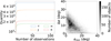Fig. 2 Left panel: cumulative distribution of absolute magnitudes determined filter by filter, shown in different colors. Right panel: heat map showing the distribution of minimum α and the total range of the phase angle covered by the objects with measured absolute magnitudes in at least one filter.

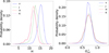Fig. 3 Distributions of computed quantities. Distributions of H (left panel) and $G_{12}^{\ast }$ (right panel). Y is shown as the blue line, J is shown in green, H is shown in red, and K is shown in purple.

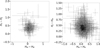Fig. 4 Small body color-color plots. The left panel shows HH − HK vs. HY − HJ, while the right panel shows HH − HK vs. HJ − HH.

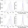Fig. 5 Distributions of absolute magnitudes and linear phase coefficients. The top panels were obtained using the full range of α. The bottom panels were obtained using α > 9.5 deg. The left column shows the absolute magnitude distributions. The right column shows the distributions of β. Y is shown as the blue line, J is shown in green, H is shown in red, and K is shown in purple.

4.2 Impact of photometric model choice

After inspecting the solutions obtained with the ${\mathrm{H}\mathrm{G}}_{12}^{\ast }$ model, we decided to test the simpler linear model of the form $$M_{\lambda }=H_{l\lambda }+{\beta }_{\lambda }\alpha ,$$(5)

where H_lλ is the absolute magnitude and β_λ is the phase coefficient in units of magnitude per degree. It is not only the simplicity of the model that is attractive (and its possibly larger number of valid solutions and quicker computation), but also the fact that we do not expect a strong OE in the NIR. Therefore, we ran the same input database with the linear model, obtaining results in at least one filter for 12 394 (more than 500 more objects than using the ${\mathrm{H}\mathrm{G}}_{12}^{\ast }$ model) and with all four valid absolute magnitudes for 180 objects, 37 more than above. The increase does not seem large, but it implies a 5% increase in the first number and a 20% increase for all valid absolute magnitudes.

The top right panel of Figure 5 shows the β_λ distribution. Despite the apparent similarities of all β distributions, the Kruskal-Wallis test gives p_value = 0.024, rejecting the null hypothesis that all median values are the same. The Dunn test indicates that the β_Y and β_J distributions differ from the β_H and β_K distributions. All distributions have median values of 0.03 mag per deg, being relatively thin and accepting a few negative values, with barely any strong outliers (11 in Y, 32 in J, 51 in H, and 30 in K with |β_λ| > 1.5 mag per deg). The H_λ distributions peak at 15.51 (Y), 13.22 (J), 12.23 (H), and 12.20 (K) (top left panel). The negative values of β may not be related to the scattering properties of the surfaces, and their explanation probably comes from macroscopic reasons such as an unfortunate sampling of the rotational light curve, or faint comet-like activity (Alvarez-Candal et al. 2016; Ayala-Loera et al. 2018).

We evaluated the impact of using the different photometric models on the estimated absolute magnitudes, creating H_l − H plots (shown in Fig. 6). The difference in the absolute magnitude per filter is shown against the value of the corresponding β. All figures follow the same pattern, strongly influenced by the linear model’s correlation between β and H_l. The median difference in the Y and J filters is about 0.28, while in the H and K filters it is about 0.3 mag. The horizontal lines show the range in magnitudes span by 90% of the sample: ΔH_Y ∈ [−0.27, 1.00], ΔH_J ∈ [−0.62, 1.38], ΔH_H ∈ [−0.94, 1.70], and ΔH_K ∈ [−0.71, 1.49]. In all cases, the corresponding β_λ values fall within −0.15 and 0.20 mag per degree (ignoring a few outliers). These numbers can be interpreted in two different ways: (i) although the linear approximation is a good proxy to estimate the absolute magnitude in NIR filters, some effects are still not included in this simplistic model, or (ii) the linear model produces systematically fainter absolute magnitudes (Fig. 6). Note that the difference in the absolute magnitudes is a measure of the OE, which is usually measured as the difference between the nonlinear phase curve and a linear fit (e.g., Slyusarev et al. 2025).

To find out if the ${\mathrm{H}\mathrm{G}}_{12}^{\ast }$ model might have been overfitting the curves and producing an unreal OE, we directly compared the resulting models with the input magnitudes. Therefore, we performed two tests. The first one shows the difference between the observed and the ${\mathrm{H}\mathrm{G}}_{12}^{\ast }$-modeled magnitudes (see Fig. 7, where the plot is cut at α = 40 deg to remove one point at approximately 80 deg that skews the figure; the same applies to Fig. 8). We computed the root mean square (RMS) of each phase curve, obtaining median values of 0.01, 0.02, 0.03, and 0.03 in the Y, J, H, and K filters, respectively. The RMS in the second test, observed minus linear-modeled magnitudes, is slightly lower (0.004, 0.01, 0.01, and 0.01, respectively) (Fig. 8), which may point to an overall better description of the observed data by linear phase curves.

Figures 7 and 8 display a black line in each panel, representing a smoothed version of the data (computed as the median value of each 21-point interval) to highlight any potential relationship between the differences in magnitudes and the phase angle. Note that in the cases of Fig. 7, there seems to be a residual signal in the smoothed line, particularly in the Y filter. These signals do not appear to be present in the panels of Fig. 8, which supports the idea that in the NIR filters, the photometric phase curves behave more linearly with less prominence of the OE.

Therefore, we are inclined to accept hypothesis (ii) mentioned above: that the linear model produces fainter magnitudes because the ${\mathrm{H}\mathrm{G}}_{12}^{\ast }$ model applied to NIR data seems to overestimate the OE region, producing brighter absolute magnitudes. Among the reasons behind these results is that we have poor coverage of the OE region, as only about 12% of the input observations were obtained with α < 5 deg. While this may seem like a substantial amount, it is essential to note that not all of these observations were utilized. Filtering by objects with valid solutions, we find that about 10% of the objects have at least two data points below 5 deg, while fewer than 3% have at least three data points with α < 5 deg; thus, the coverage of the OE region tends to be scarce as well. A dedicated program with a few select objects providing dense coverage will be instrumental in this regard.

We also checked the relation between the phase coefficients. In Fig. 9, we show $G_{12}^{\ast }$ versus β in all filters. In the plots, the data are shown as colored symbols. In contrast, the continuous black line shows a running median window taken every 11 points to highlight the apparent correlation between the two samples. The Spearman coefficient is greater than 0.5 in all cases, and the p_value ≈ 0 strongly indicates the presence of correlations. In all cases, the behavior is alike: β is about 0 deg per mag until $G_{12}^{\ast }$ is about 0.5, then it increases until β ≈ 0.08 mag per deg at $G_{12}^{\ast }$ ≈ 0.9, and then it remains almost constant for the remaining range. Note, however, that there is a considerably lower density of points in the regions of almost constant behavior of β. Figs. 6 and 9 indicate that it may be possible to estimate the values of phase coefficients from the ${\mathrm{H}\mathrm{G}}_{12}^{\ast }$ model (more time-consuming) using the linear approximation (faster computation).

Our last test was designed to verify the phase curves for a restricted range of phase angles, specifically targeting observations that lack data at low phase angles, to assess the impact on data fitting. We ran our code with the same setup as above, removing all data below α = 9.5 deg. We expect that this selection of minimum phase angle should not significantly impact our estimates, as we are dealing in the linear regime of the phase curves (Belskaya & Shevchenko 2000). After running the code, we obtained 4 749 objects with at least one absolute magnitude and 114 with all four values. The complete breakdown of the numbers is shown in Table 3. We call the absolute magnitude and phase coefficients H_e and β_e, respectively.

The distribution of H_e is similar, though low in absolute numbers, to the one shown in Fig. 3 (see Fig. 5, bottom right panel). The median values of H_λ are 15.65 (Y), 13.64 (J), 12.59 (H), and 12.56 (K). In the right panel of Fig. 5, we show the β_e distributions; they look similar to the full range of α. The median values are slightly different than those in the fullrange case (0.031, 0.032, 0.027, and 0.029) mag per deg for (Y, J, H, and K), respectively. The Kruskal-Wallis test does not reject the null hypothesis; therefore, we assume that all distributions are similar. The outliers are 5, 12, 18, and 15, respectively (|β_e| > 1.5 mag per deg).

We confirm that the difference of using the complete α range or the α > 9.5 deg is minimal: the median difference is on the order of 10⁻⁴ ‰, or less, noting that >60% of objects have at least a datum below 9.5 deg. In all filters, 90% of the results are within |(H_l − H_e)| < 3.0 mag (see Fig. 10), except in the H filter this goes up to |(H_l − H_e)| < 4.6 mag. Note that the large uncertainties in the y axis (median value of 1.3 mag) reflect the wide P(H, β) that we obtain with our method rather than an estimate of precision. The large difference between using the two models comes from objects with a low number of observations, whereby removing one datum below 9.5 degrees produces a large variation in the slope of the phase curve and, therefore, the estimated absolute magnitude. Therefore, in principle, having a restricted range of α should not strongly impact the estimation of the absolute magnitude because the linear model is well adapted for this. The same is indicated for the phase coefficients, as is displayed in Fig. 11. We conclude that using a linear model to fit data with α > 9.5 should not differ significantly from doing so with a complete range of phase angles for NIR data.

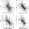Fig. 6 Scatter plots showing the difference in the absolute magnitudes computed using the ${\mathrm{H}\mathrm{G}}_{12}^{\ast }$ model (H) and the linear model (Hl) versus the linear phase coefficient (β). The dashed red lines indicate where 90% of the results lie.

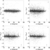Fig. 7 Comparison between measured and modeled magnitudes using the ${\mathrm{H}\mathrm{G}}_{12}^{\ast }$ model. Different panels show data in different filters. The continuous line indicates a running median of 21 points. Typical error bars in the y axis are shown in the lower right corner for reference.

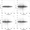Fig. 8 Comparison between measured and modeled magnitudes using the linear model. Different panels show data in different filters. The continuous line indicates a running median of 21 points. Typical error bars in the y axis are shown in the lower right corner for reference.

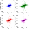Fig. 9 Scatter plots showing $G_{12}^{\ast }$ vs. β. Y is shown in blue symbols, J is shown in green, H is shown in red, and K is shown in purple. The continuous black line represents a running median window of 11 points, highlighting the relationship between the two sets. Error bars are not shown for clarity. The median error in $G_{12}^{\ast }$ ≈ 0.5, and in β ≈ 0.04 mag per deg.

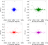Fig. 10 Comparison between Hl and He as a function of β. Different panels and colors indicate different filters: Y is shown in blue symbols, J in green, H in red, and K in purple. The error bars are not shown for clarity. The typical error on the x axis is 0.06 mag per deg, while it is about 1.3 mag on the y axis.

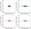Fig. 11 Same as Fig. 10, but comparing β and βe as a function of β. The typical error in the x axis is 0.06 mag per deg, while it is about 0.08 mag per deg in the y axis.

4.3 Phase coloring

Recent results point out that the usually nicknamed phase reddening effect is a coloring effect that may go either way in affecting the colors (and therefore the reflectances Ayala-Loera et al. 2018; Alvarez-Candal 2024b; Wilawer et al. 2024; Colazo et al. 2025). However, these works dealt with phase curves in the visible spectrum. We extend the analysis into the near infrared with our new results. In this part of the work, whenever reading H_λ it should be understood as H_lλ, unless explicitly mentioned otherwise. We obtained remarkably similar results to those reported in Ayala-Loera et al. (2018) for trans-Neptunian objects and Alvarez-Candal et al. (2022b) for asteroids. In these cases, the authors restricted the phase angle range to that accessible by TNOs and Centaurs, whereas in our case we used the linear model with no limit on phase angle coverage.

The figures above indicate that redder objects at opposition tend to become bluer with an increasing phase angle, while neutral-to-blue objects tend to become redder with an increasing phase angle. As was discussed in the works mentioned, we do not yet have a definite answer as to why this happens. However, we are making strides in understanding that porosity, packing, and wavelength dependence of the albedo may be behind it. These results are valid within the range of α where the models were fit, and, accepting the limitations of a simple linear model, there is evidence of a general phase coloring effect, rather than just phase reddening.

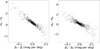Fig. 12 Colors versus relative phase coefficients. The left panel shows Y − J, while the right panel shows H − K. Error bars are not shown for clarity.

4.4 Uncertainties

To understand the uncertainty budget of our results, it is necessary to grasp where they come from: (i) We combined four different catalogs with different depths, photometric filters (Fig. 1), and photometric systems (AB vs. Vega). Regarding the depth, there is not much we can do; the objects whose data could be combined have already been combined. The transformations between filters and systems were described in Sect. 2 and the estimated offsets were given in the same section. The most affected data is in the Y filter, with a difference of roughly 0.6 mag between MOVIS and DES, while the JHK data conversions have an impact of about 0.05 mag. (ii) Data are snapshots at different epochs, and we do not know the rotational phase at which they were taken. To account for these unknown rotational phases, we applied a Monte Carlo sorting technique from a probability distribution, P(Δm), for all asteroids with a wide full width at half maximum (usually about 0.5 mag, see Fig. 2 in Alvarez-Candal 2024b) and a total range of about three mag. (iii) Finally, there are some effects that we are not including in our modeling, such as the changing aspect angle and different apparitions (as in Robinson et al. 2024 or Carry et al. 2024). Nevertheless, our approach utilizes the light-curve amplitudes from Warner et al. (2019), which include data from different apparitions and phase angles. Thus, our probability distributions, P_A(Δm), average out this effect on a large basis.

4.5 Whether these results can be used with Euclid data

The Euclid mission will map about 15 000 sq. deg of the sky, using a particular set of YJH filters, observing in almost quadrature with the Sun (solar elongation about 90 deg). This implies that the serendipitous observations of small bodies will occur at relatively large phase angles in the main belt (α ≈ 18.5 deg at about 3 AU Carry 2018; Euclid Collaboration 2025). Therefore, estimating absolute magnitudes with a restricted phase-angle coverage is crucial. In Sect. 4.2 we showed that the linear model works well even if no data is present below 9.5 deg, but in the Euclid data case, we are far from that region; therefore, our results may not hold due to the limited phase angle coverage. On the other hand, due to the observational strategy, it will be rare for the same object to be observed more than once. Additionally, Euclid’s photometric system differs from those described in this section.

Nevertheless, using our results to estimate absolute magnitudes from a single Euclid observation may still be possible. Let us assume an observation with J_euclid = 15.0 ± 0.1 at α = 18.5 deg. From the results shown above, we can create the prior p(H_l, β) using J-filter data and the linear model. For this exercise, we assumed that the MOVIS photometric system (our chosen reference) is identical to Euclid’s. We computed the posterior probability $$p(H_l,\beta \mid J_{euclid})\propto p(J_{euclid}\mid H_l,\beta )p(H_l,\beta ),$$(6)

where p(J_euclid|H_l, β) is the probability of measuring J_euclid from our model. We used a Gaussian likelihood to estimate our posterior probability and disregard the normalization factor, which is irrelevant in this case.

The resulting values of H_euclid and β_euclid are estimated as the median of the marginal distributions of p(H_l, β|J_euclid), and the uncertainty margins as the 16th and 84th percentiles (see Fig. 13). We obtained H_euclid = ${13.2}_{-1.8}^{+1.6}$ and β_euclid = ${0.040}_{-0.065}^{+0.055}$ mag per deg. These values, despite the large uncertainties, show that it is possible to estimate absolute magnitudes from a single Euclid Consortium observation at large α when a suitable prior is available.

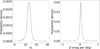Fig. 13 Marginal distributions of p(Hl, β|Jeuclid). Left: absolute magnitudes. Right: phase coefficients.

5 Conclusions

In this work, we computed absolute magnitudes in NIR filters, Y, J, H, and K, for >10 000 small bodies. The methodology used was established elsewhere; therefore, our absolute magnitudes and phase coefficients accurately represent the phase curves of these objects. Our results indicate that a linear function can accurately describe the phase curves and that it is unnecessary to use complex, nonlinear models, which may overestimate the OE, resulting in brighter absolute magnitudes than the actual ones (see also Appendix B). Because a linear function represents the curves well, the impact of using a limited range in phase angle (for instance, using α > 9.5 deg) is minimal.

On the other hand, we also confirm the effect of phase coloring happening in the NIR. The same behavior is observed in the visible for asteroids and trans-Neptunian objects, which is detected in NIR photometry: redder (bluer) objects at opposition tend to become bluer (redder) with increasing phase angles. Indeed, the relations shown in Fig. 12 reflect the linear model used; the shape would be different if other photometric models were employed, such as those in Alvarez-Candal (2024b). Unfortunately, the number of objects with NIR magnitudes is comparatively small when seen against photometric surveys in the visible. Note that we needed to join four catalogs to reach a critical mass (results for >10 000 objects) and remain an order of magnitude (at least) below any survey in the visible. The results presented in this work confirm that the data from the Euclid Consortium can be transformed into absolute magnitudes using a simple linear model and our results as prior information, provided that a conversion between the photometric systems is known.

Data availability

Data in Table 2 are available at the CDS via https://cdsarc.cds.unistra.fr/viz-bin/cat/J/A+A/701/A231 and at https://osf.io/cfxq2 unformatted plus auxiliary files. All figures in this work can be reproduced using the Google Colab Notebook https://colab.research.google.com/drive/1NIjqIpwAYj8e7t8ggp94CDD_cb4Yqqy2?usp=sharing.

Acknowledgements

AAC acknowledges financial support from the Severo Ochoa grant CEX2021-001131-S funded by MCIN/AEI/10.13039/501100011033. AAC, JLR, MC, RD, and DM acknowledge financial support from the Spanish project PID2023-153123NB-I00, funded by MCIN/AEI. MC was supported by grant No. 2022/45/B/ST9/00267 from the National Science Centre, Poland. This publication makes use of data products from the Two Micron All Sky Survey, which is a joint project of the University of Massachusetts and the Infrared Processing and Analysis Center/California Institute of Technology, funded by the National Aeronautics and Space Administration and the National Science Foundation. This project used public archival data from the Dark Energy Survey (DES). Funding for the DES Projects has been provided by the U.S. Department of Energy, the U.S. National Science Foundation, the Ministry of Science and Education of Spain, the Science and Technology FacilitiesCouncil of the United Kingdom, the Higher Education Funding Council for England, the National Center for Supercomputing Applications at the University of Illinois at Urbana-Champaign, the Kavli Institute of Cosmological Physics at the University of Chicago, the Center for Cosmology and Astro-Particle Physics at the Ohio State University, the Mitchell Institute for Fundamental Physics and Astronomy at Texas A&M University, Financiadora de Estudos e Projetos, Fundação Carlos Chagas Filho de Amparo à Pesquisa do Estado do Rio de Janeiro, Conselho Nacional de Desenvolvimento Científico e Tecnológico and the Ministério da Ciência, Tecnologia e Inovação, the Deutsche Forschungsgemeinschaft, and the Collaborating Institutions in the Dark Energy Survey. The Collaborating Institutions are Argonne National Laboratory, the University of California at Santa Cruz, the University of Cambridge, Centro de Investigaciones Energéticas, Medioambientales y Tecnológicas-Madrid, the University of Chicago, University College London, the DES-Brazil Consortium, the University of Edinburgh, the Eidgenössische Technische Hochschule (ETH) Zürich, Fermi National Accelerator Laboratory, the University of Illinois at Urbana-Champaign, the Institut de Ciències de l’Espai (IEEC/CSIC), the Institut de Física d’Altes Energies, Lawrence Berkeley National Laboratory, the Ludwig-Maximilians Universität München and the associated Excellence Cluster Universe, the University of Michigan, the National Optical Astronomy Observatory, the University of Nottingham, The Ohio State University, the OzDES Membership Consortium, the University of Pennsylvania, the University of Portsmouth, SLAC National Accelerator Laboratory, Stanford University, the University of Sussex, and Texas A&M University. Based in part on observations at Cerro Tololo Inter-American Observatory, National Optical Astronomy Observatory, which is operated by the Association of Universities for Research in Astronomy (AURA) under a cooperative agreement with the National Science Foundation. This research has made use of the SVO Filter Profile Service “Carlos Rodrigo”, funded by MCIN/AEI/10.13039/501100011033/ through grant PID2023-146210NB-I00. This work used https://www.python.org/, https://numpy.org (Harris et al. 2020), https://www.scipy.org/, Matplotlib (Hunter 2007), and https://scikit-posthocs.readthedocs.io. The text was revised using Grammarly and double-checked by the authors.

Appendix A Summary of conversions and solar colors

• 2MASS to MOVIS

  J_M = J₂ − 0.077(J − H)₂,

  H_M = H₂ + 0.032(J − H)₂,

  K_M = K₂ + 0.010(J − K)₂.

  Solar Colors: (J − H)₂ = 0.286 and (J − K)₂ = 0.362.

• UHS to 2MASS

  J₂ = J_U + 0.065(J − H)_U,

  H₂ = H_U + 0.030 − 0.070(J − H),

  K₂ = K_U − 0.010(J − K)_U,

  Solar Colors: (J − H)_U = 0.35 and (J − K)_U = 0.40.

• DES to MOVIS

  Y_M = Y_D − 0.6

Appendix B Direct comparisons

We directly compared absolute magnitudes obtained with the ${\mathrm{H}\mathrm{G}}_{12}^{\ast }$ and linear systems vs. the number of observations per object (Fig. B.1). There is a large spread, reaching values as high as about 60 % of the difference in extreme cases, especially for a low number of observations. Still, we checked that 90 % of the data (black curve in the figure) is always less than 25–30 %, and smaller in the case of the Y filter (maximum spread about 13 %). From the figures, it is also clear that the ${\mathrm{H}\mathrm{G}}_{12}^{\ast }$ absolute magnitude overestimates the value with respect to the linear model by 2 to 3 %, possibly because it tries to fit the OE region.

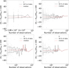Fig. B.1 $(H_l-H_{H{G}_{12}^{\ast }})/H_{H{G}_{12}^{\ast }}\times 100$ vs. number of observations. Each panel is labeled with the filter name. The continuous black line indicated the limits of 90% of the data, while the red dot-dashed line indicated the median curve.

Next, we make the same comparison, but with the α_min, i.e., the minimum phase angle observed per object. Figure B.2 shows the results. The black lines have a median spread between 15 and 20 %, depending on the filter used (smaller for Y, larger for H), and the median values of the difference are about 2.5 to 3 %, as seen above. In this plot, we can see that systematically, the median curve (in red) tends to increase with increasing α_min, implying that the linear absolute magnitudes are less bright than the ${\mathrm{H}\mathrm{G}}_{12}^{\ast }$ ones. This behavior may be expected if the ${\mathrm{H}\mathrm{G}}_{12}^{\ast }$ model is overestimating the OE: Whenever there is data at low-α the linear and the ${\mathrm{H}\mathrm{G}}_{12}^{\ast }$ model do not depart too much from each other, but in the absence of data below 5 to 7 deg, the ${\mathrm{H}\mathrm{G}}_{12}^{\ast }$ model may tend to over-fit the OE region, producing brighter absolute magnitudes.

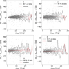Fig. B.2 $(H_l-H_{H{G}_{12}^{\ast }})/H_{H{G}_{12}^{\ast }}\times 100$ vs. αmin. Each panel is labeled with the filter name. The continuous black line indicated the limits of 90% of the data, while the red dot-dashed line indicated the median curve.

References

All Tables

All Figures

	Fig. 1 Transmission curves of all filters in the NIR used in this work. Different colors label different filters, and different line styles indicate different instruments. The different labels are 2 for 2MASS, M for MOVIS, D for DES, and U for UHS.
In the text

	Fig. 2 Left panel: cumulative distribution of absolute magnitudes determined filter by filter, shown in different colors. Right panel: heat map showing the distribution of minimum α and the total range of the phase angle covered by the objects with measured absolute magnitudes in at least one filter.
In the text

	Fig. 3 Distributions of computed quantities. Distributions of H (left panel) and $G_{12}^{\ast }$ (right panel). Y is shown as the blue line, J is shown in green, H is shown in red, and K is shown in purple.
In the text

	Fig. 4 Small body color-color plots. The left panel shows HH − HK vs. HY − HJ, while the right panel shows HH − HK vs. HJ − HH.
In the text

	Fig. 5 Distributions of absolute magnitudes and linear phase coefficients. The top panels were obtained using the full range of α. The bottom panels were obtained using α > 9.5 deg. The left column shows the absolute magnitude distributions. The right column shows the distributions of β. Y is shown as the blue line, J is shown in green, H is shown in red, and K is shown in purple.
In the text

	Fig. 6 Scatter plots showing the difference in the absolute magnitudes computed using the ${\mathrm{H}\mathrm{G}}_{12}^{\ast }$ model (H) and the linear model (Hl) versus the linear phase coefficient (β). The dashed red lines indicate where 90% of the results lie.
In the text

	Fig. 7 Comparison between measured and modeled magnitudes using the ${\mathrm{H}\mathrm{G}}_{12}^{\ast }$ model. Different panels show data in different filters. The continuous line indicates a running median of 21 points. Typical error bars in the y axis are shown in the lower right corner for reference.
In the text

	Fig. 8 Comparison between measured and modeled magnitudes using the linear model. Different panels show data in different filters. The continuous line indicates a running median of 21 points. Typical error bars in the y axis are shown in the lower right corner for reference.
In the text

	Fig. 9 Scatter plots showing $G_{12}^{\ast }$ vs. β. Y is shown in blue symbols, J is shown in green, H is shown in red, and K is shown in purple. The continuous black line represents a running median window of 11 points, highlighting the relationship between the two sets. Error bars are not shown for clarity. The median error in $G_{12}^{\ast }$ ≈ 0.5, and in β ≈ 0.04 mag per deg.
In the text

	Fig. 10 Comparison between Hl and He as a function of β. Different panels and colors indicate different filters: Y is shown in blue symbols, J in green, H in red, and K in purple. The error bars are not shown for clarity. The typical error on the x axis is 0.06 mag per deg, while it is about 1.3 mag on the y axis.
In the text

	Fig. 11 Same as Fig. 10, but comparing β and βe as a function of β. The typical error in the x axis is 0.06 mag per deg, while it is about 0.08 mag per deg in the y axis.
In the text

	Fig. 12 Colors versus relative phase coefficients. The left panel shows Y − J, while the right panel shows H − K. Error bars are not shown for clarity.
In the text

	Fig. 13 Marginal distributions of p(Hl, β|Jeuclid). Left: absolute magnitudes. Right: phase coefficients.
In the text

	Fig. B.1 $(H_l-H_{H{G}_{12}^{\ast }})/H_{H{G}_{12}^{\ast }}\times 100$ vs. number of observations. Each panel is labeled with the filter name. The continuous black line indicated the limits of 90% of the data, while the red dot-dashed line indicated the median curve.
In the text

	Fig. B.2 $(H_l-H_{H{G}_{12}^{\ast }})/H_{H{G}_{12}^{\ast }}\times 100$ vs. αmin. Each panel is labeled with the filter name. The continuous black line indicated the limits of 90% of the data, while the red dot-dashed line indicated the median curve.
In the text

References

- Alvarez-Candal, A. 2024a, Planet. Space Sci., 251, 105970 [Google Scholar]
- Alvarez-Candal, A. 2024b, A&A, 685, A29 [NASA ADS] [CrossRef] [EDP Sciences] [Google Scholar]
- Alvarez-Candal, A., Pinilla-Alonso, N., Ortiz, J. L., et al. 2016, A&A, 586, A155 [NASA ADS] [CrossRef] [EDP Sciences] [Google Scholar]
- Alvarez-Candal, A., Benavidez, P. G., Campo Bagatin, A., & Santana-Ros, T. 2022a, A&A, 657, A80 [NASA ADS] [CrossRef] [EDP Sciences] [Google Scholar]
- Alvarez-Candal, A., Jimenez Corral, S., & Colazo, M. 2022b, A&A, 667, A81 [NASA ADS] [CrossRef] [EDP Sciences] [Google Scholar]
- Ayala-Loera, C., Alvarez-Candal, A., Ortiz, J. L., et al. 2018, MNRAS, 481, 1848 [NASA ADS] [CrossRef] [Google Scholar]
- Belskaya, I. N., & Shevchenko, V. G. 2000, Icarus, 147, 94 [NASA ADS] [CrossRef] [Google Scholar]
- Bernardinelli, P. H., Bernstein, G. M., Sako, M., et al. 2022, ApJS, 258, 41 [NASA ADS] [CrossRef] [Google Scholar]
- Bowell, E., & Lumme, K. 1979, Colorimetry and Magnitudes of Asteroids, 132 [Google Scholar]
- Carruba, V., Camargo, J. I. B., Aljbaae, S., et al. 2024, MNRAS, 527, 6495 [Google Scholar]
- Carry, B. 2018, A&A, 609, A113 [NASA ADS] [CrossRef] [EDP Sciences] [Google Scholar]
- Carry, B., Peloton, J., Le Montagner, R., Mahlke, M., & Berthier, J. 2024, A&A, 687, A38 [NASA ADS] [CrossRef] [EDP Sciences] [Google Scholar]
- Casagrande, L., Ramírez, I., Meléndez, J., & Asplund, M. 2012, ApJ, 761, 16 [NASA ADS] [CrossRef] [Google Scholar]
- Colazo, M., Duffard, R., & Weidmann, W. 2021, MNRAS, 504, 761 [NASA ADS] [CrossRef] [Google Scholar]
- Colazo, M., Oszkiewicz, D., Alvarez-Candal, A., et al. 2025, Icarus, 436, 116577 [Google Scholar]
- Dark Energy Survey Collaboration (Abbott, T., et al.) 2016, MNRAS, 460, 1270 [Google Scholar]
- Euclid Collaboration (Mellier, Y., et al.) 2025, A&A, 697, A1 [Google Scholar]
- González-Fernández, C., Hodgkin, S. T., Irwin, M. J., et al. 2017, MNRAS, 474, 5459 [Google Scholar]
- Hapke, B. W. 1963, J. Geophys. Res., 68, 4571 [NASA ADS] [CrossRef] [Google Scholar]
- Harris, C. R., Millman, K. J., van der Walt, S. J., et al. 2020, Nature, 585, 357 [NASA ADS] [CrossRef] [Google Scholar]
- Hodgkin, S. T., Irwin, M. J., Hewett, P. C., & Warren, S. J. 2009, MNRAS, 394, 675 [CrossRef] [Google Scholar]
- Hunter, J. D. 2007, Comput. Sci. Eng., 9, 90 [NASA ADS] [CrossRef] [Google Scholar]
- Mahlke, M., Carry, B., & Denneau, L. 2021, Icarus, 354, 114094 [Google Scholar]
- Morrison, S. G., Strauss, R. H., Trilling, D. E., et al. 2024, AJ, 168, 180 [Google Scholar]
- Muinonen, K. 1989, Appl. Opt., 28, 3044 [NASA ADS] [CrossRef] [Google Scholar]
- Muinonen, K., Belskaya, I. N., Cellino, A., et al. 2010, Icarus, 209, 542 [Google Scholar]
- Oszkiewicz, D., Muinonen, K., Bowell, E., et al. 2011, JJQSRT, 112, 1919 [Google Scholar]
- Penttilä, A., Shevchenko, V. G., Wilkman, O., & Muinonen, K. 2016, Planet. Space Sci., 123, 117 [Google Scholar]
- Popescu, M., Licandro, J., Morate, D., et al. 2016, A&A, 591, A115 [NASA ADS] [CrossRef] [EDP Sciences] [Google Scholar]
- Robinson, J. E., Fitzsimmons, A., Young, D. R., et al. 2024, MNRAS, 531, 304 [Google Scholar]
- Sanchez, J. A., Reddy, V., Nathues, A., et al. 2012, Icarus, 220, 36 [CrossRef] [Google Scholar]
- Shevchenko, V. G., Belskaya, I. N., Muinonen, K., et al. 2016, Planet. Space Sci., 123, 101 [Google Scholar]
- Skrutskie, M. F., Cutri, R. M., Stiening, R., et al. 2006, AJ, 131, 1163 [NASA ADS] [CrossRef] [Google Scholar]
- Slyusarev, I., Shevchenko, V., Belskaya, I., et al. 2025, Planet. Space Sci., 260, 106103 [Google Scholar]
- Sykes, M. V., Cutri, R. M., Fowler, J. W., et al. 2000, Icarus, 146, 161 [NASA ADS] [CrossRef] [Google Scholar]
- Sykes, M. V., Cutri, R. M., Skrutskie, M. F., et al. 2020, 2MASS Asteroid and Comet Survey V1.0 [Google Scholar]
- Vereš, P., Jedicke, R., Fitzsimmons, A., et al. 2015, Icarus, 261, 34 [CrossRef] [Google Scholar]
- Warner, B., Pravec, P., & Harris, A. P. 2019, Asteroid Lightcurve Data Base (LCDB) V3.0, NASA Planetary Data System, Available at psi.edu/pds/resource/lc.html [Google Scholar]
- Wilawer, E., Muinonen, K., Oszkiewicz, D., Kryszczyńska, A., & Colazo, M. 2024, MNRAS, 531, 2802 [NASA ADS] [CrossRef] [Google Scholar]
- Willmer, C. N. A. 2018, ApJS, 236, 47 [Google Scholar]
In this context, each line corresponds to a different observation.
In this work, we do not use the data of the ≈ 800 trans-Neptunian objects detected by Bernardinelli et al. (2022).
Except for the linear α > 9.5 case, where we limited the minimum Δα = 3 deg to have a statistically significant number of objects.