| Issue |
A&A
Volume 701, September 2025
|
|
|---|---|---|
| Article Number | A22 | |
| Number of page(s) | 6 | |
| Section | Astrophysical processes | |
| DOI | https://doi.org/10.1051/0004-6361/202554701 | |
| Published online | 01 September 2025 | |
Cygnus X-3 as a semi-hidden PeVatron
1
Institutt for fysikk, NTNU, Trondheim, Norway
2
Department of Physics, School of Natural Sciences, Technical University Munich, Garching, Germany
⋆ Corresponding author
Received:
22
March
2025
Accepted:
18
June
2025
Abstract
Context. The high-mass X-ray binary Cygnus X-3 has long been suggested to be a source of high-energy photons and neutrinos.
Aims. In view of the increased sensitivity of current experiments, we examined the acceleration and interactions of high-energy cosmic rays (CRs) in this binary system, assuming that the compact object is a black hole.
Methods. Using a test-particle approach in a Monte Carlo framework, we employed magnetic reconnection or second-order Fermi acceleration and diffusive shock acceleration as the basic CR acceleration mechanisms.
Results. We found that in all three scenarios, CRs can be accelerated beyond PeV energies. High-energy photons and neutrinos are produced as secondaries in photo-hadronic interactions of CRs on X-ray photons and in the scattering on gas from the wind of the companion star. Normalising the predicted photon flux to the excess flux observed by LHAASO at energies above PeV in the direction of Cygnus X-3, a CR acceleration efficiency of 10−3 is sufficient to power the required CR luminosity. Our results suggest that the PeV photon flux from Cygnus X-3 could be in a bright phase that is significantly increased relative to the average flux of the past years.
Key words: acceleration of particles / astroparticle physics / radiation mechanisms: non-thermal
© The Authors 2025
 Open Access article, published by EDP Sciences, under the terms of the Creative Commons Attribution License (https://creativecommons.org/licenses/by/4.0), which permits unrestricted use, distribution, and reproduction in any medium, provided the original work is properly cited.
This article is published in open access under the Subscribe to Open model. This email address is being protected from spambots. You need JavaScript enabled to view it. to support open access publication.
1. Introduction
Cygnus X-3 is a high-mass X-ray binary in the direction of the Cygnus OB association. It has had an outstanding impact on the development of gamma-ray astronomy. In 1983, Samorski & Stamm found a periodically modulated flux of neutral particles with energies above 2 × 10¹⁵ eV coincident with Cygnus X-3 in archival data from the Kiel air-shower array. This apparent detection and the supporting evidence provided during the following years by various experiments operating in the northern hemisphere triggered an enormous theoretical interest in this source (Gaisser & Stanev 1985; Berezinsky et al. 1985, 1986). More importantly, these early results on Cygnus X-3 stimulated the building of air-shower arrays designed specifically for gamma-ray astronomy. None of these newly built arrays, such as CASA-MIA1 and SPASE2, detected a signal from Cygnus X-3, however (for a review of these early results, see Protheroe 1994). Moreover, theoretical arguments suggested that most of these claims, in particular, those by underground experiments, were erroneous, as discussed by Berezinsky et al. (1986). Still, it is a tantalising option that the initial claims for a photon signal were correct. In this case, Cygnus X-3 might have been the first PeVatron, i.e. a source able to accelerate CRs beyond PeV energies, detected. Morever, Cygnus X-3 might have been in a bright phase in the early 1980s that ended before the start of data-taking of the following generation of experiments. A strong variability like this is consistent with the decrease by at least a factor of 100 that was reported in the long-term average flux between the mid-1970s and mid-1980s (Bhat et al. 1986).
About 40 years later, the advent of advanced air-shower arrays with improved hadron-photon separation power started a new era in very-high energy gamma-ray astronomy. In particular, LHAASO3 has detected high-energy photons with energies up to few petaelectronvolt (PeV) in the direction of the Cygnus X superbubble (LHAASO Collaboration 2024). Moreover, the measured photon flux from the central region of the bubble is enhanced, with two out of eight PeV photons located inside a region of radius 0.5°. This excess corresponds to a flux that is increased by a factor of 5–10 compared to the average from the Cygnus superbubble and indicates additional point sources in this central region. The aim of this work is to examine if, and under which conditions, Cygnus X-3, which is located in the central region of the Cygnus superbubble, may cause this excess PeV photon flux.
Using a phenomenological test-particle approach, we employ different mechanisms for the acceleration of cosmic rays (CRs) depending on the level of magnetisation in the jet: In the strong magnetic turbulence close to the black hole (BH), we assumed that second-order Fermi acceleration or magnetic reconnection are efficient acceleration processes, while we suppose that diffusive shock acceleration (DSA) operates in the environment with a low magnetisation at the termination shock of the two jets that emanate from the BH. We performed simulations for two states of Cygnus X-3 that differ among others by the spectral energy distribution of X-ray photons. In the first simulation, called S1, the jet switched on right after the quiescent state and interacted with the surrounding medium close to the BH. In the second simulation, called S2 and suggested by Koljonen et al. (2023) as a promising state for the production of high-energy secondaries, the jet was on for some time and worked against the Wolf-Rayet medium, where it formed a cocoon and a termination shock. Thus, the soft X-ray state S1 is most likely disk-dominated, while the hard X-ray state S2 corresponds to a corona or jet-dominated state. We simulated the acceleration and interactions of CRs in a Monte Carlo framework that included both hadronic and photo-hadronic interactions. For the high-energy photons that are produced as secondaries in these interactions, we included absorption via pair production in the photon fields.
The plan of this paper is as follows: We start in Section 2 with a brief description of Cygnus X-3, summarising our choice for the values of the relevant physical parameters that enter in the following calculations. Then, we describe in Section 3 the acceleration scenarios we assumed to operate in Cygnus X-3 and the Monte Carlo scheme we employed to follow the time evolution of the particles. Finally, we present in Section 4 the resulting timescales of the relevant acceleration, interactions, and energy-loss processes, and our numerical results for the fluxes of high-energy photons and neutrinos. We discuss the results and the underlying assumptions before we conclude.
2. Environment of Cyg X-3
2.1. Binary system
The determination of radial velocity curves for the Cygnus X-3 binary system is complicated by strong optical extinction and the difficult separation of wind features from those arising in the photosphere of the companion. Therefore, the individual masses of the components, MCO of the compact object and MWR of the companion Wolf-Rayet (WR) star have remained uncertain so far. The published results span a wide range, from a BH with a mass close to or above 20 M⊙ (Schmutz et al. 1996; Hjalmarsdotter et al. 2008) down to upper limits of 3.6 M⊙ (Stark & Saia 2003). In contrast, the mass ratio of the binary stars can be constrained more precisely as MCO/MWR = 0.24 ± 0.06 by combining radial velocity curves derived from FeXXVI emission lines with infrared HeI absorption lines (Hanson et al. 2000). Several parameters that are important for determining the spectra of high-energy particles depend rather weakly on the masses of the binary system, fortunately. For instance, the orbital separation a, which in turn influences the target density of stellar photons and the gas in the stellar wind, only depends as a ∝ (MCO + MWR)1/3 on the total mass of the binary system. To facilitate the comparison with earlier studies, we used values close to the upper mass range discussed in the literature, setting MCO = MBH = 20 M⊙ and MWR = 50 M⊙, which corresponds to the high-mass solution of Szostek & Zdziarski (2008). We discuss the change in our results below when these masses are reduced. The Schwarzschild radius of the BH therefore was Rs = 6 × 106 cm, the orbital separation of the stars in the binary system was a = 3 × 1011 cm, and we used 9.6 kpc as the distance to Cygnus X-3 (Reid & Miller-Jones 2023).
2.2. Wind.
The gas in the stellar wind of its WR companion provides an important target for the production of secondary particles in hadronic collisions. Mass conservation implies for the density profile of a spherically symmetric wind
 (1)
(1)
where we used Ṁwind = 0.6 × 10⁻⁵ M⊙/yr and as the wind velocity vW = 2 × 108 cm/s (Szostek & Zdziarski 2008; Vilhu et al. 2021). For a proton-rich environment, μ ≃ 1, and for a helium-rich environment, as first suggested by van Kerkwijk et al. (1992), this it is μ ≃ 4.
2.3. Photon fields.
Another important target for the production of secondary particles are background photons from the stellar light of the WR star, from thermal emission of the accretion disk of the BH, and from the synchrotron corona. These photon fields lead in photo-hadronic interactions to the production of secondary photons and neutrinos, and they provide a target for the fragmentation of helium nuclei into nucleons via photo-dissociation. For the thermal photons from the WR star, we used a Planck distribution with the temperature T = 105 K, which we rescaled as (RWR/r)2 at the distance r to the WR star with radius RWR = 6 × 1010 cm (Sahakyan et al. 2014).
The accretion rate Ṁ in an X-ray binary may be strongly time-dependent, implying that the nature of the accretion disk and thus the temperature profile of the disk varies as well. We were mainly interested in the bright phase of Cygnus X-3 with accretion close to the Eddington rate and therefore used a geometrically thin and optically thick Keplerian accretion disk (Shakura & Sunyaev 1973; Chakrabarti 1996). In this case, the thermal emission from the accretion disk is described by the temperature profile
![Mathematical equation: $$ \begin{aligned} T(r) = \left( \frac{3GM\dot{M}}{8\sigma \pi r^3} \left[ 1-(R_0/r)^{1/2} \right] \right)^{1/4}. \end{aligned} $$](/articles/aa/full_html/2025/09/aa54701-25/aa54701-25-eq2.gif) (2)
(2)
Since the radial extension of the disk is rather small, the total emission is close to a Planck distribution with T(r)≃T(R0). For a helium-rich composition and the standard value η = 0.1 for the accretion efficiency  , the Eddington luminosity becomes LEdd ≃ 2.6 × 1038(MBH/M⊙) erg/s, which in turn fixes Ṁ = λṀEdd for a chosen λ. The observed X-ray luminosity favours a high value of λ and MBH (Veledina 2024). We calculated the density of disk photons at a given point in the jet by integrating the photon emissivity into the corresponding solid angle dΩ over the accretion disk (Cerutti et al. 2011), choosing λ = 0.5 and as smallest radius R0 of the acceleration and of the emission region six Schwarzschild radii, R0 = 6Rs ≃ 3.6 × 107 cm, while we set Rout = 10Rs for the outer radius of the disk.
Finally, we fixed the spectral density of the X-ray photons in the corona. We identified the emission zone in which energetic electrons are accelerated and radiated these photons via synchrotron and inverse-Compton scattering with the acceleration region of hadrons. Then, we used the INTEGRAL4 measurements from Cangemi et al. (2021) for the quiet-state S1 and for the state S2 to determine the spectral number density of X-ray photons in the range 10–100 keV. In order to connect them to observations in the radio range from AMI-LA5 and RATAN6 (Piano et al. 2012), we assumed an additional break at E = 1 eV. For the size of the emission region, we assumed L = 8RS in the case of S1 and L = tanϑRS2, with RS2 = 7 × 1011 cm as the distance to the termination shock and ϑ = 12° as the jet opening angle (Mioduszewski et al. 2001; Spencer et al. 2022).
The resulting spectral number density of stellar, accretion disk, and X-ray photons are shown in Fig. 1 for states S1 (left panel) and S2 (right panel).
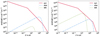 |
Fig. 1. Spectral density of the photon backgrounds in states S1 (left) and S2 (right). |
2.4. Magnetic field.
As the radial profile for the magnetic field strength around the BH, we used
 (3)
(3)
setting B0 = 2.1 × 10⁷ G at the jet injection point r0 = 10Rs ≃ 6 × 107 cm (Miller-Jones et al. 2004). The slope δ is rather uncertain, with 0.5 ≤ δ ≤ 0.83 being considered by Miller-Jones et al. We followed Koljonen et al. (2018), who argued that δ ≃ 0.65 fits the data best.
In addition to the field strength, the ratio of the energy density in the magnetic field and the total energy density of the plasma is an important parameter. This ratio, the so-called magnetisation σm = B2/(4πρ) with ρ ≃ nγmc2 as the enthalpy density, becomes of order one at r ≃ 1011 cm. Since the Alfvén velocity  approaches the speed of light for σm ≫ 1, the borderline between weak and strong magnetisation also separates the parameter space in which DSA is more efficient than acceleration by second-order Fermi process or magnetic reconnection.
3. Theoretical framework
3.1. Acceleration scenarios
Various phenomenological models have been proposed to explain the observed gamma-ray emission from Cygnus X-3. Several models connected the gamma-ray emission to particle acceleration in shocks, either generated internally in the jets or externally at the recollimination or the termination of the jet (Romero et al. 2003; Piano et al. 2012; Baerwald & Guetta 2013). If these shocks are collisionless, DSA can lead to particle acceleration. Estimates for the velocity of the outflow in Cygnus X-3 range from non-relativistic (β = v/c < 0.3; Waltman et al. 1996) to mildly relativistic (β = 0.63; Miller-Jones et al. 2004 and β > 0.81; Mioduszewski et al. 2001), indicating time-dependent jet velocities. These trans-relativistic flows with  are well suited for fast acceleration if the magnetisation σm is small. Thus, we assumed that DSA only operates at a large enough distance, r ≳ 1011 cm, from the BH, such that σm ≲ 1. In the Bohm diffusion limit,
  , the acceleration rate of a particle with rigidity
  is given by (Lagage & Cesarsky 1983)
 (4)
(4)
With ζ ≃ 10 − 20 for a parallel shock, (vsh/c)2 ≃ 0.1, we conservatively set η = 10−3. We assumed shock velocities vsh that were low enough for relativistic effects such as beaming or a large loss-cone of CRs at shock crossing to be neglected.
An alternative acceleration process that has recently attracted increased attention is magnetic reconnection. This acceleration mechanism was applied to micro-quasars in general by de Gouveia Dal Pino & Lazarian (2005) and to Cygnus X-3 by Khiali et al. (2015). In this model, magnetic reconnection occurs in current sheets that are produced when field lines arising from the accretion disk and of the BH magnetosphere meet. If the reconnection velocity is fast enough, trapped particles between the two converging magnetic fluxes of opposite polarity can gain energy in a similar way to the first-order Fermi process, leading to (Kowal 2012)
 (5)
(5)
with vA as the Alfvén velocity, and Lrec as the extension of the reconnection zone. In this scenario, the acceleration region is close to the BH, at a distance between ≃6RS and ≃10RS. As a result, the photon fields as potential targets for photo-hadronic interactions are much more intense than in the DSA case. Moreover, the magnetisation is very strong, and we thus assume that DSA is not effective.
Finally, we considered as an alternative to magnetic reconnection second-order Fermi acceleration in the strong magnetic turbulence close to the BH. For σm ≫ 1 and thus vA ≃ c, the efficiency of second-order Fermi acceleration is not suppressed relative to DSA. Moreover, the slope of the produced particle distributions can potentially becomeuniversal, with α ∼ 2.1 found by Comisso et al. (2024), and acceleration rate
 (6)
(6)
Here, κ is an efficiency factor determined by Comisso & Sironi (2019) using PIC simulations as κ ∼ 0.1, |u|=Γ|β|∼1 is the spatial part of the four-velocity of the scattering centers, and Lc is the coherence length of the turbulent magnetic field. We assumed that the energy of the magnetic turbulence is mainly contained in large-scale modes and used Lc = 106 cm for the numerical estimate. Thus, these two processes for the chosen parameters roughly lead to the same maximum energy (see the left panel of Fig. 2) and to the same secondary production. Second-order Fermi acceleration has the advantage, however, that it can also operate at larger distances from the BH as long as the jet is strongly magnetised. Since at larger distances both the acceleration efficiency and the secondary production would be reduced, the results from this accelerationmechanism would interpolate between those of magnetic reconnection very close to the BH and DSA at the termination shock. We therefore considered only these two extreme cases in our simulation.
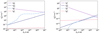 |
Fig. 2. Rates for synchrotron losses |


3.2. Monte Carlo scheme
We used a leaky-box scheme in which for a chosen time step Δt the escape probability of a charged particle with energy E from the acceleration region was first calculated,
![Mathematical equation: $$ \begin{aligned} p_{\rm esc}= 1-\exp [ (1-\alpha )\ln (1+\xi ) ] . \end{aligned} $$](/articles/aa/full_html/2025/09/aa54701-25/aa54701-25-eq18.gif) (7)
(7)
Here, α is the theoretically predicted slope of the differential energy spectrum of accelerated particles in the case of no interactions and energy losses, which we chose for both acceleration mechanisms as α = 2.3, while ξ = (dE/dt)accΔt/E is the energy fraction gained according to Eqs. (4) and (5). If the particle stays in the acceleration process, the true energy gain is calculated as the sum of the acceleration gain and the continuous energy losses, [(dE/dt)acc − (dE/dt)CEL]Δt, where the latter include synchrotron and, for muons, inverse-Compton losses. Finally, it is decided if the particle decays or interacts: First, the probability that something happens is compared to a random number r that is uniformly distributed in [0 : 1[, then, a second random number r is compared to the branching ratios for the relevant decay and interactionchannels.
When a photo-hadronic interactions occured, we used the modified version of the SOPHIA program (Mucke et al. 2000) developed by Kachelrieß et al. (2008) to generate secondary particles, while we employed QGSJET-IIc (Ostapchenko 2011, 2013) for hadronic interactions. We took the finite decay time of all unstable particles into account except for neutral pions and only included stable charged all particles in the acceleration process. For the decay of unstable particles, we employed SIBYLL (Fletcher et al. 1994).
After the particles escaped from the acceleration region, we assumed that the magnetic field strength is weak enough for them to move ballistically. Except for photons, the interaction depth is small, τ ≪ 1, and multiple interactions can be neglected. Thus, we added after escape a final interaction for hadrons with a probability p = 1 − exp(−τ) and let all unstable particles decay. In the case of photons, we calculated the pair-production probability on background photons in the direction of the observer. In addition, we added the pair-production probability on photons of the cosmic microwave background (CMB) and the extragalactic background light from Franceschini et al. (2008) to obtain the final flux observed on Earth, F = F0exp(−τγγ). We neglected the absorption on the starlight in the Milky Way, which adds only a minor correction relative to the absorption on the CMB (Vernetto & Lipari 2016) and the effect of electromagnetic cascades, which is well justified above the pair-production threshold, Eγ ≃ (1 − 10) GeV.
The acceleration time is much shorter than the orbital period of the system. Thus, there is an orbital modulation of the fluxes, both because the interaction depth varies with the orbital phase, and also for photons because the absorption probability changes. In the energy range in which we are mainly interested, (1014–1016) eV, the modulation is only minor, however: The photon absorption probability is dominated by the CMB, while the interaction depths only varies by a factor of a few (see Lammert 2025 for details). We therefore present results for the average fluxes below.
4. Numerical results
We start to discuss the case of magnetic reconnection and DSA assuming that protons are injected into the acceleration process, as was the common assumption in previous works. As the material close to the BH originates from the helium-rich wind of the WR companion star, we then briefly discuss the case of helium as CR primaries.
4.1. Proton injection
After we specified the acceleration mechanisms and the physical parameters determining interaction and energy loss processes, we compared the resulting acceleration, interaction, and energy loss rates. This allowed us to confirm and to interpret the numerical results from our Monte Carlo simulations. In Fig. 2 we show these rates for protons7, and we compare (left panel) the case of acceleration by reconnection in state S1 to the case of DSA in state S2 (right panel). The dense photon fields close to the BH mean that photo-hadronic interactions are the most important energy-loss process. They limit the maximum energy of protons in the reconnection case to ≃6 × 10¹⁶ eV. Hadronic interactions on gas from the stellar wind of the WR star play a negligible role during the acceleration phase, even for an increased gas density close to the BH, as assumed by Khiali et al. (2015). In the case of DSA in state S2, synchrotron losses and photo-hadronic interactions are equally important, but the former slightly more so. The maximum energy of protons is somewhat lower, ≃3 × 10¹⁶ eV, but still high enough to expect secondaries with energies above PeV. In both cases, the Hillas criterium allows higher CR rigidities than the interaction and energy losses: In S1, the Hillas criterium allows for rigidities up to 300 PV, for instance.
We normalised the fluxes such that the CR luminosity satisfied LCR = ηCRλLEdd ≃ 3.9 × 1038 erg/s, that is, we assumed optimistically that 15% of the available energy is used to accelerate hadrons. In Fig. 3 we show the rescaled flux E2Φ = E2dN/(dAdtdE) of CR protons (blue line), of the sum of all neutrino flavours (orange line), and of photons (red line) as function of energy E. In addition to the proton flux after interactions, the presumed power-law E−2.3 and the flux escaping the acceleration region are presented. The high-energy cutoffs agree with the expectations from Fig. 2, that is, a rather soft suppression above 8 × 10¹⁶ eV in state S1 and a sharper suppression above 2 × 10¹⁶ eV in state S2. Similarly, the secondary fluxes in state S1 are higher, as expected, than in state S2. At energies above 1014 eV pair production on CMB photons dominates, while at lower energies, the absorption on stellar photons becomes important.
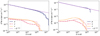 |
Fig. 3. Particle fluxes of CR protons, sum of all neutrino flavours, and photon fluxes as function of energy E for the case of reconnection in state S1 (left) and DSA in state S2 (right). |
In Fig. 4 we show a close-up of the photon fluxes, where we split the flux into two components, depending on their production inside or outside the acceleration zone. The outer component is mainly produced in hadronic interactions, and thus, the slope of this component repeats the slope of the proton flux at an energy a factor that is ≃20 higher. In addition, we show in Fig. 4 the gamma-ray flux measured by LHAASO in the direction of the Cygnus X superbubble from LHAASO Collaboration (2024). Cygnus X-3 only contributes a fraction, mostly at the highest energies, of the total flux from the Cygnus superbubble. Since no detailed information on the exposure is published, we can only roughly estimate the integrated flux Φ(> E) from the central region above PeV energies as Φ(> PeV)=N/(AT)≃9 × 10−14/(m2s) using as effective area A ≃ 106m2 from Ma et al. (2022), T ≃ 6000 h for 3 years of data taking, and N = 2 events above PeV. This corresponds to a photon flux of about E2Φ(E = PeV)≃10−11 GeV/cm2s. Thus, the obtained photon flux, which in both states is on the level E2Φ(E = PeV)≃10−9 GeV/cm2s, should be scaled down by 10−2, which would reduce the required CR acceleration efficiency to ηCR ∼ 10−3. At this level, the photon flux would be well below the lower limits from the MAGIC collaboration (Aleksić et al. 2010). The correspondingly down-scaled neutrino flux is a factor of 100 below the 90% C.L. upper limit set by the IceCube collaboration (Abbasi et al. 2022). Even for ηCR = 0.1, the number of expected muon neutrino events/year in IceCube above 10 TeV is only about one in S1 and two in S2.
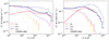 |
Fig. 4. Photon fluxes as a function of energy E for the case of reconnection in state S1 (left) and by DSA in state S2 (right) compared to the gamma-ray flux measured by LHAASO (LHAASO Collaboration 2024) in the direction of the Cygnus X superbubble. |
4.2. Helium injection
Next, we briefly discuss the case of helium as CR primaries. Since the acceleration and diffusion of CRs only depends on rigidity, the rates given in Eqs. (4) and (5) apply directly to helium. As synchrotron losses for the same primary energy scale with (q/m)4, the losses of helium are reduced by a factor of 16. In the case of hadronic interactions, the He-He cross section is a larger by a factor of 6–7 than the proton-proton cross section, while the number of targets is reduced by a factor of 4 for a fixed wind density ρ. Thus, the secondary production due to hadronic interactions is increased by a factor 1.5–1.75 relative to the proton case discussed before. The differences are more pronounced in the case of interactions with background photons. In addition to the usual photo-hadronic channel, the photo dissociation of helium nuclei into nucleons sets in at a threshold energy here that is ≃10 times lower. Thus, helium nuclei at the highest energies will fragment into nucleons, resulting in the same energy cutoff as obtained in the proton case. At lower energies, mainly helium nuclei will escape from the acceleration zone, leading to a somewhat increased secondary production. Since the interaction depth is shallow, the largest part of the accelerated helium nuclei escapes and contributes to the helium part of the Galactic CR spectrum.
5. Discussion
We now briefly review some of our main assumptions. In this section, we discuss the change in our results when we modify them.
-
Our values for the masses of the binary stars are at the higher end of the range discussed in the literature, and the choice MBH = 5 M⊙ and MWR = 20 M⊙ would be more in line with the analysis of Koljonen & Maccarone (2017), for example. This value for MBH would increase the temperature of the accretion disk by only ∼30%, and we showed that the disk photons play only a minor role as target. More importantly, the number density of X-ray photons in state S1 would increase by a factor ≃43 = 64, which would reduce the maximum energy in the S1 state by a factor of about 10. This reduction in the maximum proton energy would mean that Cygnus X-3 is barely a PeV photon source in the S1 state. Alternatively, a two-zone model would have to be considered in which the X-ray emission is partly decoupled from the acceleration of hadrons.
-
The accretion rate Ṁ regulates the total amount of available power, of which the fraction ηCRλ can be channelled into the acceleration of CRs. X-ray observations favour super-Eddington accretion rates and/or a rather massive BH (Veledina 2024). Moreover, radio observations showed a very large variability in the radio flux (Gregory et al. 1972; Green et al. 2025). If this variability is connected to variations in Ṁ or ηCR, then the PeV photon flux should be in a one-zone model correlated with the variation in the radio band. If, on the other hand, a smaller jet-opening angle and higher jet velocities are characteristic for flares (Spencer et al. 2022), then the PeV photon flux in state S2 might be anti-correlated to the radio flares.
-
In state S2, a combined scenario with both DSA at the recollimination or termination shock and second-order Fermi throughout the jet or magnetic reconnection close to the BH is possible. In particular, for a lower value of δ, the maximum achievable energy in DSA is reduced, and this region would not contribute to high-energy photons. It might still be the main contributor to the X-ray emission via leptonic processes, however. Hence, this case would be a realisation of a two-zone model in which the target density for photo-hadronic interactions is strongly reduced, and rather low BH masses would be unproblematic even for the acceleration via reconnection close to the BH.
-
We neglected relativistic beaming effects. As the flux scales with the Doppler factor δ as δ3, already modest gamma factors could lead to a strong increase of the observed photon fluxes.
-
We considered a purely hadronic model for the photon emission of Cygnus X-3, without trying to self-consistently explain the X-ray emission by electrons. A combined model in which the acceleration of electrons and hadrons is simulated based on the same mechanism would help us to constrain physical parameters such as the magnetic field strength and the size of the acceleration region, but this is deferred to a future work.
6. Conclusions
We have examined the acceleration and interactions of high-energy CRs in the high-mass X-ray binary Cygnus X-3, motivated by the recent observations of two PeV photons in the direction of Cygnus X-3. We found that in all the three acceleration scenarios we considered (magnetic reconnection, second-order Fermi acceleration on magnetic turbulence, and diffusive shock acceleration), CRs can be accelerated beyond PeV energies. In the hadronic scenario we studied, high-energy photons are mainly produced in interactions with gas from the wind of the WR companion star. The CR luminosity to explain the excess flux observed by LHAASO at energies above PeV energies is rather low, requiring a CR acceleration efficiency of 10−3–10−2. This suggests that the PeV photon flux from Cygnus X-3 might be in a bright phase that is significantly increased relative to the average flux of the past years.
The Chicago Air Shower Array (CASA) combined with the Michigan Muon Array (MIA).
The South Pole Air Shower Experiment.
The Large High Altitude Air Shower Observatory.
The INTErnational Gamma-Ray Astrophysics Laboratory.
The Arcminute Microkelvin Imager Large Array.
The Soviet RATAN-600 Radio Telescope.
See Lammert (2025) for a discussion of other long-lived particles.
Acknowledgments
We would like to thank Karri Koljonen for useful discussions and helpful comments on the draft, and Egor Podlesnyi for help in estimating the expected number of IceCube events. M.K. is grateful to the late Venya Berezinsky for introducing him to the story of Cygnus X-3 in the 1980s.
References
- Abbasi, R., Ackermann, M., Adams, J., et al. 2022, ApJ, 930, L24 [NASA ADS] [CrossRef] [Google Scholar]
- Aleksić, J., Antonelli, L. A., Antoranz, P., et al. 2010, ApJ, 721, 843 [Google Scholar]
- Baerwald, P., & Guetta, D. 2013, ApJ, 773, 159 [Google Scholar]
- Berezinsky, V. S., Bugaev, E. V., & Zaslavskaya, E. S. 1985, JETP Lett., 42, 528 [Google Scholar]
- Berezinsky, V. S., Castagnoli, C., & Galeotti, P. 1986, ApJ, 301, 235 [Google Scholar]
- Berezinsky, V. S., Ellis, J. R., & Ioffe, B. L. 1986, Phys. Lett. B, 172, 423 [Google Scholar]
- Bhat, C. L., Sapru, M. L., & Razdan, H. 1986, ApJ, 306, 587 [Google Scholar]
- Cangemi, F., Rodriguez, J., Grinberg, V., et al. 2021, A&A, 645, A60 [NASA ADS] [CrossRef] [EDP Sciences] [Google Scholar]
- Cerutti, B., Dubus, G., Malzac, J., et al. 2011, A&A, 529, A120 [NASA ADS] [CrossRef] [EDP Sciences] [Google Scholar]
- Chakrabarti, S. K. 1996, Phys. Rept., 266, 229 [Google Scholar]
- Comisso, L., & Sironi, L. 2019, ApJ, 886, 122 [Google Scholar]
- Comisso, L., Farrar, G. R., & Muzio, M. S. 2024, ApJ, 977, L18 [Google Scholar]
- de Gouveia Dal Pino, E. M., & Lazarian, A. 2005, A&A, 441, 845 [CrossRef] [EDP Sciences] [Google Scholar]
- Fletcher, R. S., Gaisser, T. K., Lipari, P., & Stanev, T. 1994, Phys. Rev. D, 50, 5710 [Google Scholar]
- Franceschini, A., Rodighiero, G., & Vaccari, M. 2008, A&A, 487, 837 [NASA ADS] [CrossRef] [EDP Sciences] [Google Scholar]
- Gaisser, T. K., & Stanev, T. 1985, Phys. Rev. Lett., 54, 2265 [Google Scholar]
- Green, D. A., Rhodes, L., & Bright, J. 2025, Res. Notes AAS, 9, 35 [Google Scholar]
- Gregory, P. C., Kronberg, P. P., Seaquist, E. R., et al. 1972, Nature, 239, 440 [Google Scholar]
- Hanson, M. M., Still, M. D., & Fender, R. P. 2000, ApJ, 541, 308 [Google Scholar]
- Hjalmarsdotter, L., Zdziarski, A. A., Larsson, S., et al. 2008, MNRAS, 384, 278 [NASA ADS] [CrossRef] [Google Scholar]
- Kachelrieß, M., Ostapchenko, S., & Tomàs, R. 2008, Phys. Rev. D, 77, 023007 [Google Scholar]
- Khiali, B., de Gouveia Dal Pino, E. M., & del Valle, M. V. 2015, MNRAS, 449, 34 [Google Scholar]
- Koljonen, K. I. I., & Maccarone, T. J. 2017, MNRAS, 472, 2181 [NASA ADS] [CrossRef] [Google Scholar]
- Koljonen, K. I. I., Maccarone, T., McCollough, M. L., et al. 2018, A&A, 612, A27 [NASA ADS] [CrossRef] [EDP Sciences] [Google Scholar]
- Koljonen, K. I. I., Satalecka, K., Lindfors, E. J., & Liodakis, I. 2023, MNRAS, 524, L89 [NASA ADS] [Google Scholar]
- Kowal, G., & de Gouveia Dal Pino, E. M., & Lazarian, A. 2012, Phys. Rev. Lett., 108, 241102 [NASA ADS] [CrossRef] [Google Scholar]
- Lagage, P. O., & Cesarsky, C. J. 1983, A&A, 125, 249 [NASA ADS] [Google Scholar]
- Lammert, E. 2025, Master’s Thesis, TU München [Google Scholar]
- LHAASO Collaboration (Cao, Z., et al.) 2024, Sci. Bull., 69, 449 [NASA ADS] [CrossRef] [Google Scholar]
- Ma, X.-H., Bi, Y.-J., Cao, Z., et al. 2022, Chin. Phys. C, 46, 030001 [CrossRef] [Google Scholar]
- Miller-Jones, J. C. A., Blundell, K. M., Rupen, M. P., et al. 2004, ApJ, 600, 368 [NASA ADS] [CrossRef] [Google Scholar]
- Mioduszewski, A. J., Rupen, M. P., Hjellming, R. M., Pooley, G. G., & Waltman, E. B. 2001, ApJ, 553, 766 [Google Scholar]
- Mucke, A., Engel, R., Rachen, J. P., Protheroe, R. J., & Stanev, T. 2000, Comput. Phys. Commun., 124, 290 [CrossRef] [Google Scholar]
- Ostapchenko, S. 2011, Phys. Rev. D, 83, 014018 [Google Scholar]
- Ostapchenko, S. 2013, EPJ Web Conf., 52, 02001 [Google Scholar]
- Piano, G., Tavani, M., Vittorini, V., et al. 2012, A&A, 545, A110 [NASA ADS] [CrossRef] [EDP Sciences] [Google Scholar]
- Protheroe, R. J. 1994, ApJS, 90, 883 [Google Scholar]
- Reid, M. J., & Miller-Jones, J. C. A. 2023, ApJ, 959, 85 [CrossRef] [Google Scholar]
- Romero, G. E., Torres, D. F., Bernado, M. M. K., & Mirabel, I. F. 2003, Astron. Astrophys., 410, L1 [Google Scholar]
- Sahakyan, N., Piano, G., & Tavani, M. 2014, ApJ, 780, 29 [Google Scholar]
- Samorski, M., & Stamm, W. 1983, ApJ, 268, L17 [CrossRef] [Google Scholar]
- Schmutz, W., Geballe, T. R., & Schild, H. 1996, A&A, 311, L25 [Google Scholar]
- Shakura, N. I., & Sunyaev, R. A. 1973, A&A, 24, 337 [NASA ADS] [Google Scholar]
- Spencer, R. E., Garrett, M., Bray, J. D., & Green, D. A. 2022, MNRAS, 512, 2618 [Google Scholar]
- Stark, M. J., & Saia, M. 2003, ApJ, 587, L101 [Google Scholar]
- Szostek, A., & Zdziarski, A. A. 2008, MNRAS, 386, 593 [Google Scholar]
- van Kerkwijk, M. H., Charles, P. A., Geballe, T. R., et al. 1992, Nature, 355, 703 [NASA ADS] [CrossRef] [Google Scholar]
- Veledina, A., et al. 2024, Nat. Astron., 8, 1031 [NASA ADS] [CrossRef] [Google Scholar]
- Vernetto, S., & Lipari, P. 2016, Phys. Rev. D, 94, 063009 [NASA ADS] [CrossRef] [Google Scholar]
- Vilhu, O., Kallman, T. R., Koljonen, K. I., & Hannikainen, D. C. 2021, A&A, 649, A176 [NASA ADS] [CrossRef] [EDP Sciences] [Google Scholar]
- Waltman, E. B., Foster, R. S., Pooley, G. G., Fender, R. P., & Ghigo, F. D. 1996, AJ, 112, 2690 [NASA ADS] [CrossRef] [Google Scholar]
All Figures
|
Fig. 1. Spectral density of the photon backgrounds in states S1 (left) and S2 (right). |
| In the text | |
|
Fig. 2. Rates for synchrotron losses |
| In the text | |
|
Fig. 3. Particle fluxes of CR protons, sum of all neutrino flavours, and photon fluxes as function of energy E for the case of reconnection in state S1 (left) and DSA in state S2 (right). |
| In the text | |
|
Fig. 4. Photon fluxes as a function of energy E for the case of reconnection in state S1 (left) and by DSA in state S2 (right) compared to the gamma-ray flux measured by LHAASO (LHAASO Collaboration 2024) in the direction of the Cygnus X superbubble. |
| In the text | |
Current usage metrics show cumulative count of Article Views (full-text article views including HTML views, PDF and ePub downloads, according to the available data) and Abstracts Views on Vision4Press platform.
Data correspond to usage on the plateform after 2015. The current usage metrics is available 48-96 hours after online publication and is updated daily on week days.
Initial download of the metrics may take a while.