| Issue |
A&A
Volume 701, September 2025
|
|
|---|---|---|
| Article Number | A98 | |
| Number of page(s) | 8 | |
| Section | Astrophysical processes | |
| DOI | https://doi.org/10.1051/0004-6361/202555242 | |
| Published online | 04 September 2025 | |
Ultra-luminous X-ray pulsars as sources of TeV neutrinos
1
Institut für Astronomie und Astrophysik, Kepler Center for Astro and Particle Physics, University of Tuebingen, Sand 1, 72076 Tübingen, Germany
2
INAF – Osservatorio Astronomico di Brera, via Bianchi 46, 23807 Merate (LC), Italy
3
Faculty of Physics, University of Białystok, ul. K. Ciołkowskiego 1L, 15-245 Białystok, Poland
4
Dr. Karl Remeis Observatory, Erlangen Centre for Astroparticle Physics, Friedrich-Alexander-Universität Erlangen-Nürnberg, Sternwartstr. 7, 96049 Bamberg, Germany
⋆ Corresponding author: This email address is being protected from spambots. You need JavaScript enabled to view it.
Received:
21
April
2025
Accepted:
4
August
2025
Abstract
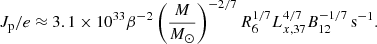
We explored the expected properties of the neutrino emission from accreting neutron stars in X-ray binaries using numerical simulations. The simulations are based on a model in which neutrinos are produced by the decay of charged pions and kaons, generated in inelastic collisions between protons accelerated up to TeV energies in the magnetosphere of a magnetized (B ∼ 1012 G) neutron star and protons of the accretion disc. Our results show that this process can produce strong neutrino emission up to a few tens of TeV when the X-ray luminosity is above ∼1039 erg s−1, as in ultra-luminous X-ray (ULX) pulsars. We show that neutrinos from a transient Galactic ULX pulsar with Lx ≈ 5 × 1039 erg s−1 can be detected with kilometre-scale detectors such as IceCube if the source is within about 3–4 kpc. We also derived an upper limit on the neutrino flux from the Galactic ULX pulsar Swift J0243.6+6124 using IceCube data, a result that has not been previously reported. Our findings establish a new benchmark for future astrophysical neutrino observations, critical for interpreting data from current and upcoming instruments with significantly improved sensitivity.
Key words: accretion / accretion disks / neutrinos / stars: neutron / X-rays: binaries / X-rays: individuals: Swift J0243.6+6124
© The Authors 2025
 Open Access article, published by EDP Sciences, under the terms of the Creative Commons Attribution License (https://creativecommons.org/licenses/by/4.0), which permits unrestricted use, distribution, and reproduction in any medium, provided the original work is properly cited.
This article is published in open access under the Subscribe to Open model. This email address is being protected from spambots. You need JavaScript enabled to view it. to support open access publication.
1. Introduction
One of the major breakthroughs in the context of multi-messenger astrophysics of the last decade was the discovery of TeV-PeV neutrinos of astrophysical origin by the IceCube neutrino observatory (Aartsen et al. 2013; IceCube Collaboration 2013; Aartsen et al. 2014a). Although the dominant contribution is from extragalactic sources, neutrino emission has recently been identified from the Galactic plane at a 4.5σ level of significance, which contributes ∼6 to 13% of the all-sky astrophysical flux at 30 TeV (Icecube Collaboration 2023). This excess is likely dominated by diffuse emission from our Galaxy, but a fraction of it could be linked to a population of unresolved point sources (e.g. Icecube Collaboration 2023; Vecchiotti et al. 2023). Some of these sources could be X-ray binaries (XRBs), which have long been considered candidates for neutrino emission (e.g. Berezinskii et al. 1985; Gaisser & Stanev 1985; Auriemma et al. 1986). XRBs are composed of a compact object (a neutron star or a black hole) and, typically, a non-degenerate companion star. X-rays are the result of the accretion of the mass lost by the companion star onto the compact object. The gravitationally captured mass sometimes forms an accretion disc. Some XRBs are persistent X-ray sources but most display variability, sometimes bright X-ray outbursts that can last several weeks followed by long periods of low X-ray luminosity or quiescence (for two recent reviews on XRBs, see, for example, Kretschmar et al. 2019; Sazonov et al. 2020).
Over the years, three primary mechanisms for neutrino production in XRBs have been identified. The first and second mechanisms involve interactions of accelerated hadrons. In the first case, high-energy protons accelerated within the XRB, such as in jets, relativistic winds, or neutron star magnetospheres, collide with protons in environments such as stellar winds, accretion discs, or the jets themselves. These collisions produce primarily pions, which decay into gamma rays and neutrinos. This mechanism has been proposed for microquasars, gamma-ray binaries, and other XRBs (e.g. Anchordoqui et al. 2003; Romero et al. 2003; Bednarek 2005; Christiansen et al. 2006; Torres & Halzen 2007; Reynoso et al. 2008; Neronov & Ribordy 2009; Sahakyan et al. 2014; Kosmas et al. 2023; Peretti et al. 2025). The second mechanism occurs when accelerated protons interact with photon fields from the accretion disc, companion star, or neutron star surface. Here, pion production is dominated by the Δ-resonance process, with subsequent decays generating neutrinos and gamma rays. The proton–photon interaction is particularly relevant for microquasars and accreting pulsars (Levinson & Waxman 2001; Distefano et al. 2002; Bednarek 2009). Neutrinos produced via these mechanisms typically lie in the GeV–PeV energy range. A third mechanism arises in accretion columns of bright, transient XRBs. High temperatures in these regions are expected to lead to electron–positron pair production, with neutrino emission occurring via pair annihilation (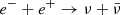 ). Additionally, neutrino synchrotron emission (
 ) contributes to the total neutrino luminosity, though its contribution is comparatively minor. These processes produce neutrinos in the MeV energy band (Mushtukov et al. 2018; Asthana et al. 2023; Mushtukov et al. 2025).
In hadronic scenarios within XRBs, gamma-ray and neutrino emission are intrinsically linked because both originate from the decay of neutral and charged pions produced in high-energy hadron interactions. However, unlike neutrinos, gamma rays are susceptible to absorption within the dense photon environments of XRBs, primarily through pair production. This process occurs when high-energy gamma rays interact with lower-energy photons from the companion star (UV radiation) and the accretion disc (X-rays). The significant absorption of gamma rays can lead to a quenched or substantially altered observed gamma-ray emission (see e.g. Torres & Halzen 2007; Neronov & Ribordy 2009; Aharonian 2011; Ducci et al. 2023). In contrast, neutrinos interact very weakly with matter and radiation and can therefore escape the dense astrophysical environments of XRBs without significant absorption. Consequently, neutrinos can provide a more direct and undistorted view of the fundamental hadronic acceleration processes occurring in these systems.
Neutrino emission from XRBs has been actively investigated using detectors such as IceCube (Abbasi et al. 2022) and the Astronomy with a Neutrino Telescope and Abyss environmental RESearch project (ANTARES; Albert et al. 2017). While intriguing excesses in neutrino event rates have been reported near sources such as Cyg X-3 in IceCube data (Koljonen et al. 2023) and in Baikal Deep Underwater Neutrino Telescope or Baikal-Gigaton Volume Detector observations (Allakhverdyan et al. 2023), no statistically significant neutrino detection has been confirmed to date. Current theoretical models predict neutrino fluxes from XRBs that remain below the sensitivity thresholds of existing detectors (Abbasi et al. 2022; Albert et al. 2017).
In this work, we extend the hadronic neutrino production mechanism proposed by Anchordoqui et al. (2003) to the broader range of mass accretion rates (or equivalently, X-ray luminosities) characteristic of highly magnetized (B ∼ 1012 G) accretion disc-fed pulsars. This mechanism relies on the hypothesis of an electrostatic gap forming in the neutron star magnetosphere. While theoretically motivated, the existence, stability, and detailed behaviour of such gaps under accretion conditions remain unconfirmed observationally and lack validation via self-consistent numerical magnetohydrodynamic or particle-in-cell simulations (see, for example, Cerutti et al. 2015, and references therein). Our refined predictions for system-specific neutrino fluxes will enable better comparisons with future observations from next-generation detectors such as IceCube-Gen2 (Grant et al. 2019) and KM3NeT (KM3NeT Collaboration 2024), whose enhanced sensitivity will provide critical tests of astrophysical neutrino models.
The paper is organized as follows: Section 2 presents the theoretical framework and model assumptions. Section 3 details the numerical simulations adopted to derive our results, which are described in Sect. 4. Concluding remarks are given in Sect. 5.
2. Model synopsis
Our calculations and simulations build on the model proposed by Anchordoqui et al. (2003), which itself extends the framework developed by Cheng & Ruderman (1989). The central idea involves electrostatic gaps forming in the neutron star magnetosphere due to differential rotation between the star and the inner accretion disc. These gaps accelerate protons to energies that can exceed 100 TeV. When these protons collide with the accretion disc, they trigger hadronic showers. Cheng & Ruderman (1989) considered the gamma-ray emission from the decay of neutral pions produced by the proton–proton collisions. Anchordoqui et al. (2003) investigated the high-energy neutrino production via charged pion decay and, to a lesser extent, charged kaons that decay into neutrinos.
The model by Anchordoqui et al. (2003) assumes a strongly shielded gap, where the magnetospheric region is devoid of X-ray photons produced by the accretion, maximizing the potential drop:
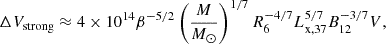 (1)
(1)
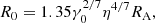
where Lx, 37 is the X-ray luminosity produced by the accretion in units of 1037 erg s−1, M is the mass of the neutron star, R6 is its radius in units of 106 cm, B12 is the magnetic field at the neutron star surface (in units of 1012 G), β = 2R0/RA, where
 (2)
(2)
 (3)
(3)
Here R0 is defined according to the work by Wang (1996), RA is the Alfvén radius, γ0 = −Bϕ0/Bz0 ≈ 1 is the magnetic pitch angle, η is the screening factor (a partially screened disc is assumed, η = 0.1)1, μ = BRNS3/2 is the dipolar magnetic moment (RNS is the radius of the neutron star), and Ṁ is the mass accretion rate. In the model of Anchordoqui et al. (2003), the electrostatic gap is situated over the accretion disc from R0 up to a distance of about RA.
Cheng & Ruderman (1991) and Cheng et al. (1992) later introduced the weakly shielded gap scenario to improve the physical realism of the model, a feature not considered by Anchordoqui et al. (2003). In the weakly shielded gap scenario, X-ray photons from the accretion column penetrate the gap, producing e± pairs that reduce the potential:
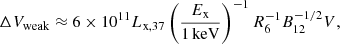 (4)
(4)
where Ex is the characteristic energy of the X-ray photons (Cheng & Ruderman 1991; Cheng et al. 1992). Weak shielding lowers proton acceleration energies compared to the strongly shielded case.
The proton current through the gap, critical for determining the neutrino flux, is given by (Cheng & Ruderman 1989)
 (5)
(5)
To simulate the hadronic processes initiated by proton–proton collisions, Anchordoqui et al. (2003) employed DPMJET-II, a Monte Carlo event generator designed for modelling high-energy hadronic interactions using Gribov-Regge theory (Ranft 1995), and Geant4, a comprehensive toolkit for simulating the passage of particles through matter, widely used in high-energy physics and applicable to astrophysical phenomena (Agostinelli et al. 2003)2. While DPMJET generated the initial proton-nucleon interactions and secondary particle spectra, Geant4 tracked the subsequent electromagnetic and hadronic shower development within the disc, including pion decays. Their simulations revealed a power-law neutrino spectrum, predicting that systems like the Be/XRB A0535+26 could emit detectable neutrino signals, highlighting the potential for multi-wavelength astrophysics to probe hadronic processes in extreme environments.
3. Numerical simulations
In our study, we focused on the weakly shielded gap scenario, which was not addressed by Anchordoqui et al. (2003), to complement and enhance their work. We assumed a mono-energetic proton beam striking the accretion disc perpendicularly near RA, with the proton energy determined by Eq. (4) and their flux by Eq. (5). For each simulation run, we generated between 104 and 106 protons in the beam and subsequently scaled the results using Eq. (5). The accretion disc was modelled as a cylindrical volume with height 2h, filled with a gas of ionized protons of density np. The density of the disc and height at ∼RA were derived using the disc structure equations from Shakura & Sunyaev (1973). For the radiation pressure dominated cases (the so-called zone A), in our simulations with Lx ≳ 1038 erg s−1 we adopted the scale-height formula reported in Bykov et al. (2022) and Mushtukov et al. (2017):  . As pointed out in Mushtukov et al. (2017, and references therein), for high values of the X-ray luminosity (higher than those assumed in our simulations), the accretion disc can become advection-dominated and the thickness given by the above formula can be overestimated. For np, we referred to the numerical calculations by Inoue et al. (2023) and Chashkina et al. (2019).
Within the disc, the interaction between the beam and target protons generates particle cascades, leading to the creation of various particle types. Our focus is on those that result in the formation of neutrinos. At the energies given to the beam protons, neutrinos are produced from the initial creation of π± and, to a lesser extent, K± mesons that emerge from the proton–proton collision and any subsequent hadronic interactions involving π± and K±, with the target protons. Neutrinos arise from the decays of these mesons, the most probable of which are
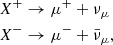
where X is π or K. Subsequently, muons can further decay, producing additional neutrinos:
In conclusion, there will be a mix of muon and electron neutrinos.
In addition to proton–proton collisions, proton–photon interactions represent another potential mechanism for meson and neutrino production in high-energy astrophysical environments. In our study, we focused exclusively on proton–proton interactions for meson production for two reasons. First, the energy threshold required for efficient meson production in proton–photon processes, particularly those involving interactions with accretion disc photons, is of the order of 102 TeV (Aharonian 2011; Neronov & Ribordy 2009). Given that the majority of proton energies explored within our simulation framework reside below this threshold, the kinematic requirements for effective proton–proton interactions are often not met. Second, the proton–photon cross-section is at least two orders of magnitude smaller than the proton–proton cross-section (e.g. Reynoso et al. 2008; Kelner & Aharonian 2008). Given the proton and photon densities in our simulations, the proton–proton channel dominates the proton–photon production process.
We performed our simulations entirely using Geant4 (version 11.3.0). This choice reflects the steady advancements in the software over the past ∼22 years, which have established the FTFP_BERT physics list3 as the recommended option for high-energy physics applications, including hadronic interactions and decays. Nevertheless, we emphasize that ongoing validation studies remain critical to assess existing models and extend the physics implementations against other particle interaction/transport codes and experimental data (see e.g. Allison et al. 2016). FTFP_BERT is optimized for the GeV to TeV energy range and includes elastic, inelastic, and capture processes for the hadronic interactions. For high-energy inelastic collisions (≳4 GeV), the Fritiof (FTF) model governs the production of high-multiplicity secondary particles, notably charged pions and kaons. These particles either undergo secondary interactions within the target (the accretion disc) or decay via electromagnetic/weak processes, producing muons and neutrinos. To quantify the neutrino flux and energy spectrum, Geant4 tracks the full decay chains of pions, kaons, and muons, while secondary hadronic interactions are modelled to account for cascade-driven modifications to the final state of the particle distributions. To optimize computational efficiency, we stopped tracking particles once their energies fell below 50 GeV. This cutoff minimizes time-consuming low-energy cascade calculations while preserving fidelity to the GeV-TeV neutrino spectrum, the primary focus of astrophysical detectors like IceCube.
The magnetic field strength at RA, given by B(RA) = B0(RNS/RA)3 (for a dipolar field with B0 at the neutron star surface), is relatively low when typical values for accreting pulsars in high-mass XRBs (a sub-class of XRBs; see e.g. van Paradijs 1998) are used. This makes synchrotron losses for π±, K±, and μ± negligible in most cases, as also shown by Anchordoqui et al. (2003). Figure 1 shows that synchrotron losses only slightly affect muons at very high X-ray luminosities (Lx ≳ 1039 erg s−1), where B(RA)≳105 G. However, in these high mass accretion regimes, np is also very high. This strongly reduces the probability that muons precursors, π± and K±, decay before inelastic collisions with protons of the disc. An example is shown in Fig. 2, which shows the probability that π± and K± decay before undergoing inelastic collisions with protons in the disc (assuming np = 5 × 1021 cm−3). Therefore, the magnetic field strength can be neglected in first approximation.
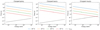 |
Fig. 1. Synchrotron cooling times for pions, kaons, and muons, for different magnetic field strengths, as a function of energy, compared to their lifetimes in the accretion disc rest frame. |
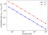 |
Fig. 2. Probability that the mean free path for decay of π± and K± is less than the mean free path for inelastic collisions with protons of the accretion disc as a function of energy, assuming np = 5 × 1021 cm−3. |
4. Results
We explored the expected intensity and spectral properties of neutrinos from a hypothetical accreting pulsar in high-mass XRBs fed by an accretion disc across an X-ray luminosity range of 5 × 1036 erg s−1 to 5 × 1039 erg s−1. The neutron star was assumed to have a magnetic field of B0 = 5 × 10¹² G, consistent with values typically observed in such systems (e.g. Staubert et al. 2019). We assumed a neutron star with mass of 1.4 M⊙ and a radius of 12 km. We further assumed that the source remains in a persistent accretion state, with no inhibition of accretion at low luminosities (Illarionov & Sunyaev 1975). The simulated neutrino spectra are parameterized using a power-law model to facilitate comparisons. For each simulation, the derived neutrino luminosities and power-law slopes are summarized in Table 1, alongside the corresponding input parameters. Figure 3 presents the neutrino luminosity (Lν) as a function of the X-ray luminosity. To account for neutrino flavour oscillations during propagation from the source to Earth, which redistribute the initial flux into approximately equal contributions of electron, muon, and tau neutrinos, the predicted neutrino luminosity was scaled by a factor of 1/3. This adjustment accounts for the focus of detectors like IceCube on track-like events from muon neutrinos, which provide far better directional precision for identifying astrophysical sources than cascade events produced by electron and tau neutrinos (Aartsen et al. 2014a, 2020).
Summary of the simulations.
 |
Fig. 3. Neutrino luminosity as a function of X-ray luminosity for each of the simulated datasets (Table 1). |
The correlation between Lν and Lx in the plot arises from the scaling of both the proton flux (Eq. (5)) and proton energy (Eq. (4)) with Lx. The sub-exponential scaling of Lν with increasing Lx is caused by the higher proton density within the accretion disc. At these densities, charged mesons (π±, K±) with energies exceeding 50 GeV experience enhanced inelastic collisions prior to decay. These interactions induce energy redistribution into secondary particle cascades, suppressing the high-energy decay products (e.g. muons and neutrinos), leading to a flatter Lν trend.
Figure 4 shows the simulated spectra where neutrino events are re-binned to a logarithmic scale (refer to Table 1). As Lx increases, the spectra become harder. This trend is primarily due to the increase in Ep with Lx. The variation in the power-law slope depends on a complex interplay among various interaction processes occurring within the accretion disc, competing with decays, as a function of the beam protons energy, target proton density, and disc thickness.
Our simulations show that pulsars in binary systems with X-ray luminosities greater than ∼1039 erg s−1 are promising neutrino emitters within the model framework presented in this work. Accreting pulsars in binary systems with such high luminosities are classified as ultra-luminous X-ray sources with pulsars (PULXs), and represent a sub-class of ultra-luminous X-ray sources (ULXs). PULXs are identified by the detection of X-ray pulsations, which confirm the presence of an accreting neutron star. In contrast, the broader ULX class includes systems thought to host stellar-mass black holes, intermediate-mass black holes, or neutron stars where pulsations have not yet been observed (e.g. King et al. 2023). Approximately 1800 ULXs have been observed in nearby galaxies (Walton et al. 2022; Middleton & King 2017; Earnshaw et al. 2019), with only a few confirmed or strong candidate PULXs (Bachetti et al. 2014; Israel et al. 2017a,b; Carpano et al. 2018; Fürst et al. 2016; Sathyaprakash et al. 2019; Rodríguez Castillo et al. 2020; Pintore et al. 2025). In addition to these, three transient pulsars in the Magellanic Clouds, SMC X-3 (Tsygankov et al. 2017), RX J0209.6-7427 (Vasilopoulos et al. 2020), and 1A 0538-66 (White & Carpenter 1978), have shown occasional outbursts exceeding LX ≈ 1039 erg s−1, along with the first Galactic PULX, Swift J0243.6+6124, discovered in 2017 (Wilson-Hodge et al. 2018, and references therein). Challenges in detecting PULXs and other transient bright accreting pulsars arise from their intermittent pulsations, low pulsed fractions, and transient nature. This suggests that the true population of PULXs, both in external galaxies and potentially in the Milky Way, is underestimated (e.g. Pintore et al. 2025; Rodríguez Castillo et al. 2020). Binary evolution models also make highly uncertain predictions for the number of ULXs with neutron stars per galaxy, with estimates depending on star formation history, metallicity, and magnetic field properties (Shao & Li 2015; Wiktorowicz et al. 2021; Kuranov et al. 2020; Kovlakas et al. 2025; King et al. 2023). For example, some models suggest that only a handful of these binary systems exist in galaxies similar to the Milky Way (e.g. Kuranov et al. 2020).
To assess neutrino observability from transient Galactic PULXs, we adopted a hypothetical source with properties similar to those of Swift J0243.6+6124. This source reached peak X-ray luminosities of LX > 1039 erg s−1 over 20 days (Doroshenko et al. 2020) and is located at ∼5 − 7 kpc (Reig et al. 2020). No neutrino detections or upper limits for this source have been reported by IceCube (see Appendix A). Given the transient nature of these systems, we followed the methodology of Abbasi et al. (2022), who compared neutrino fluence predictions for the 2015 V404 Cygni outburst (a non-PULX black hole system) to the 5σ discovery potential of IceCube. In our analysis, for a fiducial PULX with LX = 5 × 1039 erg s−1 (see Table 1 and Fig. 4), we re-scaled the IceCube discovery potential at 1 TeV from Abbasi et al. (2022) to 100 GeV, accounting for the slope of the neutrino spectrum (γ = −2.9; see Table 1) and the detector energy-dependent effective area ratio A1 TeV/A100 GeV ≈ 400 (Stettner 2019). We adopted 100 GeV as the reference energy, rather than 1 TeV, to compare the expected neutrino fluence with the 5σ discovery potential of IceCube, as this more effectively highlights the detection capabilities for sources with soft neutrino spectra, as in our case. Similarly to Anchordoqui et al. (2003), we assumed the phenomenological estimate for the beaming factor of b = ΔΩ/4π ∼ 0.1 (Cheng & Ruderman 1989). The resulting fluences, as a function of the time interval during which the source maintains an X-ray luminosity of 5 × 1039 erg s−1, are shown in Fig. 5 for three distances (2, 3, and 4 kpc), compared to the 5σ discovery potential. We note that the extragalactic PULXs with X-ray luminosities exceeding those in our test case by a factor of ∼100 have been observed (Israel et al. 2017a). If such a luminous transient were to occur in the Milky Way, its neutrino emission would be detectable at distances well beyond the 2–4 kpc range explored here. Additionally, ongoing and future upgrades to DeepCore, the sub-array of IceCube sensitive to neutrinos in the ∼10 GeV to a few TeV energy range, will enhance its sensitivity. As shown in Fig. 3 of Abbasi et al. (2022), these advancements could lower the 5σ discovery potential by approximately a factor of 3, expanding detectability prospects (see also Eller et al. 2023).
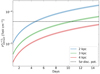 |
Fig. 5. Fluence at 100 GeV of a hypothetical PULX with LX = 5 × 1039 erg s−1 as a function of the time interval during which the source maintains this luminosity level, for three different distances. The horizontal dashed line shows the 5σ discovery potential in IceCube. |
5. Concluding remarks
We have shown that, within the framework of our model, nearby ULXs hosting neutron stars could be detectable sources of neutrinos during periods of high X-ray activity (Lx > 1039 erg s−1), provided their X-ray outbursts last long enough. Although no such sources have been observed nearby so far, their transient nature leaves open the possibility of a future discovery. The outlook for these studies is promising: upgrades of the currently active neutrino telescopes and new high-energy neutrino telescopes are either nearing completion or are planned for the next decade. Furthermore, combining data from these detectors is expected to significantly enhance sensitivity (Schumacher et al. 2025), improving our ability to observe these sources. We note a potential challenge for neutrino detection in luminous ULXs. High-resolution spectra of some ULXs, including pulsar-hosting systems, suggest outflows launched from the surface of the inner parts of the accretion disc. Such outflows may not always occur: for example, models indicate that outflows are expected to be negligible when the dipolar magnetic field is strong (B > few 1013 G; Mushtukov et al. 2019). If present, these outflows could affect the properties of the electrostatic gap, potentially suppressing it entirely. Crucially, the original gap models (Cheng & Ruderman 1989, 1991) did not account for outflow effects.
We also note that our adopted weakly shielded gap assumption accounts in principle for the reduced potential drop across the gap caused by pair production from X-ray photons (compared to the strongly shielded gap case considered in most previous works). Nonetheless, the stronger disc radiation expected in ULXs could cause an additional reduction in this potential drop. Therefore, the formation and stability of gaps under these conditions remains uncertain and should be further investigated through observations and dedicated magnetohydrodynamic or particle-in-cell simulations.
η takes into account the screening effects of the currents induced in the surface of the accretion disc.
For more information: https://geant4.web.cern.ch/
See https://renkulab.io/projects/astronomy/mmoda/icecube and the online data analysis (MMODA) service for IceCube, https://mmoda.io
Acknowledgments
We thank the referee for the useful comments. LD acknowledges funding from the Deutsche Forschungsgemeinschaft (DFG, German Research Foundation) – Projektnummer 549824807. PR acknowledges support by the “Programma di Ricerca Fondamentale INAF 2023”. This research made use of NumPy (Harris et al. 2020), SciPy (Virtanen et al. 2020), and pandas (Wes McKinney 2010).
References
- Aartsen, M. G., Abbasi, R., Abdou, Y., et al. 2013, Phys. Rev. Lett., 111, 021103 [Google Scholar]
- Aartsen, M. G., Abbasi, R., Ackermann, M., et al. 2014a, J. Instrum., 9, P03009 [Google Scholar]
- Aartsen, M. G., Ackermann, M., Adams, J., et al. 2014a, Phys. Rev. Lett., 113, 101101 [Google Scholar]
- Aartsen, M. G., Ackermann, M., Adams, J., et al. 2020, Phys. Rev. Lett., 124, 051103 [Google Scholar]
- Abbasi, R., Ackermann, M., Adams, J., et al. 2022, ApJ, 930, L24 [NASA ADS] [CrossRef] [Google Scholar]
- Agostinelli, S., Allison, J., Amako, K., et al. 2003, Nucl. Instrum. Methods Phys. Res. A, 506, 250 [Google Scholar]
- Aharonian, F. 2011, Nucl. Phys. B Proc. Suppl., 221, 5 [Google Scholar]
- Albert, A., André, M., Anton, G., et al. 2017, JCAP, 2017, 019 [CrossRef] [Google Scholar]
- Allakhverdyan, V. A., Avrorin, A. D., Avrorin, A. V., et al. 2023, MNRAS, 526, 942 [Google Scholar]
- Allison, J., Amako, K., Apostolakis, J., et al. 2016, Nucl. Instrum. Methods Phys. Res. A, 835, 186 [Google Scholar]
- Anchordoqui, L. A., Torres, D. F., McCauley, T. P., Romero, G. E., & Aharonian, F. A. 2003, ApJ, 589, 481 [NASA ADS] [CrossRef] [Google Scholar]
- Asthana, A., Mushtukov, A. A., Dobrynina, A. A., & Ognev, I. S. 2023, MNRAS, 522, 3405 [Google Scholar]
- Auriemma, G., Bilokon, H., & Grillo, A. F. 1986, Nuovo Cimento C Geophys. Space Phys. C, 9, 451 [Google Scholar]
- Bachetti, M., Harrison, F. A., Walton, D. J., et al. 2014, Nature, 514, 202 [NASA ADS] [CrossRef] [Google Scholar]
- Bednarek, W. 2005, ApJ, 631, 466 [NASA ADS] [CrossRef] [Google Scholar]
- Bednarek, W. 2009, Phys. Rev. D, 79, 123010 [Google Scholar]
- Berezinskii, V. S., Castagnoli, C., & Galeotti, P. 1985, Nuovo Cimento C Geophys. Space Phys. C, 8, 185 [Google Scholar]
- Bykov, S. D., Gilfanov, M. R., Tsygankov, S. S., & Filippova, E. V. 2022, MNRAS, 516, 1601 [NASA ADS] [CrossRef] [Google Scholar]
- Carpano, S., Haberl, F., Maitra, C., & Vasilopoulos, G. 2018, MNRAS, 476, L45 [NASA ADS] [CrossRef] [Google Scholar]
- Cerutti, B., Philippov, A., Parfrey, K., & Spitkovsky, A. 2015, MNRAS, 448, 606 [Google Scholar]
- Chashkina, A., Lipunova, G., Abolmasov, P., & Poutanen, J. 2019, A&A, 626, A18 [NASA ADS] [CrossRef] [EDP Sciences] [Google Scholar]
- Cheng, K. S., & Ruderman, M. 1989, ApJ, 337, L77 [NASA ADS] [CrossRef] [Google Scholar]
- Cheng, K. S., & Ruderman, M. 1991, ApJ, 373, 187 [NASA ADS] [CrossRef] [Google Scholar]
- Cheng, K. S., Lau, M. M., Cheung, T., Leung, P. P., & Ding, K. Y. 1992, ApJ, 390, 480 [NASA ADS] [CrossRef] [Google Scholar]
- Christiansen, H. R., Orellana, M., & Romero, G. E. 2006, Phys. Rev. D, 73, 063012 [Google Scholar]
- Distefano, C., Guetta, D., Waxman, E., & Levinson, A. 2002, ApJ, 575, 378 [Google Scholar]
- Doroshenko, V., Zhang, S. N., Santangelo, A., et al. 2020, MNRAS, 491, 1857 [Google Scholar]
- Ducci, L., Romano, P., Vercellone, S., & Santangelo, A. 2023, MNRAS, 525, 3923 [CrossRef] [Google Scholar]
- Earnshaw, H. P., Roberts, T. P., Middleton, M. J., Walton, D. J., & Mateos, S. 2019, MNRAS, 483, 5554 [NASA ADS] [CrossRef] [Google Scholar]
- Eller, P., DeHolton, K. L., Weldert, J., & Ørsøe, R. 2023, arXiv e-prints [arXiv:2307.15295] [Google Scholar]
- Fürst, F., Walton, D. J., Harrison, F. A., et al. 2016, ApJ, 831, L14 [Google Scholar]
- Gaisser, T. K., & Stanev, T. 1985, Phys. Rev. Lett., 54, 2265 [Google Scholar]
- Grant, D., Ackermann, M., Karle, A., & Kowalski, M. 2019, BAAS, 51, 288 [Google Scholar]
- Harris, C. R., Millman, K. J., van der Walt, S. J., et al. 2020, Nature, 585, 357 [NASA ADS] [CrossRef] [Google Scholar]
- IceCube Collaboration 2013, Science, 342, 1242856 [Google Scholar]
- IceCube Collaboration (Abbasi, R., et al.) 2021, arXiv e-prints [arXiv:2101.09836] [Google Scholar]
- Icecube Collaboration (Abbasi, R., et al.) 2023, Science, 380, 1338 [NASA ADS] [CrossRef] [Google Scholar]
- Illarionov, A. F., & Sunyaev, R. A. 1975, A&A, 39, 185 [NASA ADS] [Google Scholar]
- Inoue, A., Ohsuga, K., Takahashi, H. R., & Asahina, Y. 2023, ApJ, 952, 62 [NASA ADS] [CrossRef] [Google Scholar]
- Israel, G. L., Belfiore, A., Stella, L., et al. 2017a, Science, 355, 817 [NASA ADS] [CrossRef] [Google Scholar]
- Israel, G. L., Papitto, A., Esposito, P., et al. 2017b, MNRAS, 466, L48 [NASA ADS] [CrossRef] [Google Scholar]
- Kelner, S. R., & Aharonian, F. A. 2008, Phys. Rev. D, 78, 034013 [Google Scholar]
- King, A., Lasota, J.-P., & Middleton, M. 2023, New A Rev., 96, 101672 [NASA ADS] [CrossRef] [Google Scholar]
- KM3NeT Collaboration (Aiello, S., et al.) 2024, Eur. Phys. J. C, 84, 885 [CrossRef] [Google Scholar]
- Koljonen, K. I. I., Satalecka, K., Lindfors, E. J., & Liodakis, I. 2023, MNRAS, 524, L89 [NASA ADS] [Google Scholar]
- Kosmas, O., Papavasileiou, T., & Kosmas, T. 2023, Universe, 9, 517 [NASA ADS] [CrossRef] [Google Scholar]
- Kovlakas, K., Misra, D., Amato, R., & Israel, G. 2025, A&A, 694, L9 [NASA ADS] [CrossRef] [EDP Sciences] [Google Scholar]
- Kretschmar, P., Fürst, F., Sidoli, L., et al. 2019, New A Rev., 86, 101546 [NASA ADS] [CrossRef] [Google Scholar]
- Kuranov, A. G., Postnov, K. A., & Yungelson, L. R. 2020, Astron. Lett., 46, 658 [NASA ADS] [CrossRef] [Google Scholar]
- Levinson, A., & Waxman, E. 2001, Phys. Rev. Lett., 87, 171101 [Google Scholar]
- Middleton, M. J., & King, A. 2017, MNRAS, 470, L69 [Google Scholar]
- Mushtukov, A. A., Suleimanov, V. F., Tsygankov, S. S., & Ingram, A. 2017, MNRAS, 467, 1202 [NASA ADS] [Google Scholar]
- Mushtukov, A. A., Tsygankov, S. S., Suleimanov, V. F., & Poutanen, J. 2018, MNRAS, 476, 2867 [NASA ADS] [CrossRef] [Google Scholar]
- Mushtukov, A. A., Ingram, A., Middleton, M., Nagirner, D. I., & van der Klis, M. 2019, MNRAS, 484, 687 [NASA ADS] [CrossRef] [Google Scholar]
- Mushtukov, A. A., Potekhin, A. Y., Markozov, I. D., et al. 2025, MNRAS, 538, 2396 [Google Scholar]
- Neronov, A., & Ribordy, M. 2009, Phys. Rev. D, 79, 043013 [Google Scholar]
- Peretti, E., Petropoulou, M., Vasilopoulos, G., & Gabici, S. 2025, A&A, 698, A188 [NASA ADS] [CrossRef] [EDP Sciences] [Google Scholar]
- Pintore, F., Pinto, C., Rodriguez-Castillo, G., et al. 2025, A&A, 695, A238 [NASA ADS] [CrossRef] [EDP Sciences] [Google Scholar]
- Ranft, J. 1995, Phys. Rev. D, 51, 64 [CrossRef] [PubMed] [Google Scholar]
- Reig, P., Fabregat, J., & Alfonso-Garzón, J. 2020, A&A, 640, A35 [NASA ADS] [CrossRef] [EDP Sciences] [Google Scholar]
- Reynoso, M. M., Romero, G. E., & Christiansen, H. R. 2008, MNRAS, 387, 1745 [NASA ADS] [CrossRef] [Google Scholar]
- Rodríguez Castillo, G. A., Israel, G. L., Belfiore, A., et al. 2020, ApJ, 895, 60 [Google Scholar]
- Romero, G. E., Torres, D. F., Kaufman Bernadó, M. M., & Mirabel, I. F. 2003, A&A, 410, L1 [NASA ADS] [CrossRef] [EDP Sciences] [Google Scholar]
- Sahakyan, N., Piano, G., & Tavani, M. 2014, ApJ, 780, 29 [Google Scholar]
- Sathyaprakash, R., Roberts, T. P., Walton, D. J., et al. 2019, MNRAS, 488, L35 [NASA ADS] [CrossRef] [Google Scholar]
- Sazonov, S., Paizis, A., Bazzano, A., et al. 2020, New A Rev., 88, 101536 [NASA ADS] [CrossRef] [Google Scholar]
- Schumacher, L. J., Bustamante, M., Agostini, M., Oikonomou, F., & Resconi, E. 2025, arXiv e-prints [arXiv:2503.07549] [Google Scholar]
- Shakura, N. I., & Sunyaev, R. A. 1973, A&A, 500, 33 [NASA ADS] [Google Scholar]
- Shao, Y., & Li, X.-D. 2015, ApJ, 802, 131 [Google Scholar]
- Staubert, R., Trümper, J., Kendziorra, E., et al. 2019, A&A, 622, A61 [NASA ADS] [CrossRef] [EDP Sciences] [Google Scholar]
- Stettner, J. 2019, in 36th International Cosmic Ray Conference (ICRC2019), Int. Cosmic Ray Conf., 36, 1017 [NASA ADS] [Google Scholar]
- Torres, D. F., & Halzen, F. 2007, Astropart. Phys., 27, 500 [NASA ADS] [CrossRef] [Google Scholar]
- Tsygankov, S. S., Doroshenko, V., Lutovinov, A. A., Mushtukov, A. A., & Poutanen, J. 2017, A&A, 605, A39 [NASA ADS] [CrossRef] [EDP Sciences] [Google Scholar]
- van Paradijs, J. 1998, in The Many Faces of Neutron Stars, eds. R. Buccheri, J. van Paradijs, & A. Alpar, NATO Adv. Study Inst. (ASI) Ser. C, 515, 279 [NASA ADS] [CrossRef] [Google Scholar]
- Vasilopoulos, G., Ray, P. S., Gendreau, K. C., et al. 2020, MNRAS, 494, 5350 [NASA ADS] [CrossRef] [Google Scholar]
- Vecchiotti, V., Villante, F. L., & Pagliaroli, G. 2023, ApJ, 956, L44 [Google Scholar]
- Virtanen, P., Gommers, R., Oliphant, T. E., et al. 2020, Nat. Methods, 17, 261 [Google Scholar]
- Walton, D. J., Mackenzie, A. D. A., Gully, H., et al. 2022, MNRAS, 509, 1587 [Google Scholar]
- Wang, Y. M. 1996, ApJ, 465, L111 [Google Scholar]
- Wes McKinney, 2010, in Proceedings of the 9th Python in Science Conference, eds. S. van der Walt, & J. Millman, 56 [Google Scholar]
- White, N. E., & Carpenter, G. F. 1978, MNRAS, 183, 11P [Google Scholar]
- Wiktorowicz, G., Lasota, J.-P., Belczynski, K., et al. 2021, ApJ, 918, 60 [CrossRef] [Google Scholar]
- Wilson-Hodge, C. A., Malacaria, C., Jenke, P. A., et al. 2018, ApJ, 863, 9 [Google Scholar]
Appendix A: Flux upper limit determination for Swift J0243.6+6124 in the IC86_VII IceCube dataset
We used data analysis tools from the IceCube repository in Renkulab4 and SkyLLH5 to perform general maximum likelihood ratio hypothesis testing. These tools do not allow arbitrary time intervals to be selected. Instead, they rely on predefined observation periods defined by the IceCube collaboration (Icecube Collaboration 2021). Therefore, we analysed the IC86_VII dataset, which roughly corresponds to the period of the Swift J0243.6+6124 outburst. From our analysis, we obtained a test statistic (TS) of 0.008, ns = 0.36, and γ = −5. Here, TS represents the likelihood ratio between the signal-plus-background and the background-only hypotheses, ns is the best-fit estimate of the number of signal events contributing to the data, and γ characterizes the energy distribution of the signal. We calculated the significance of the source, that is, the p-value, using the appropriate SkyLLH tools. This was done by generating the TS distribution of 105 background-only data trials, which assumes zero injected signal events. The resulting p-value is 0.47, meaning that there is not significant signal detection. Assuming a spectral slope of −3 (that is, the slope obtained from our simulation for a source with Lx ≈ 1038 − 39 erg s−1), we derived a 90% confidence level flux upper limit at 1 TeV of 5.7 × 10⁻¹¹ TeV cm−2 s−1 (9.1 × 10⁻¹¹ erg cm−2 s−1).
All Tables
All Figures
|
Fig. 1. Synchrotron cooling times for pions, kaons, and muons, for different magnetic field strengths, as a function of energy, compared to their lifetimes in the accretion disc rest frame. |
| In the text | |
|
Fig. 2. Probability that the mean free path for decay of π± and K± is less than the mean free path for inelastic collisions with protons of the accretion disc as a function of energy, assuming np = 5 × 1021 cm−3. |
| In the text | |
|
Fig. 3. Neutrino luminosity as a function of X-ray luminosity for each of the simulated datasets (Table 1). |
| In the text | |
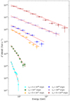 |
Fig. 4. Simulated spectra for six different scenarios (Table 1), each fitted with a power-law model. |
| In the text | |
|
Fig. 5. Fluence at 100 GeV of a hypothetical PULX with LX = 5 × 1039 erg s−1 as a function of the time interval during which the source maintains this luminosity level, for three different distances. The horizontal dashed line shows the 5σ discovery potential in IceCube. |
| In the text | |
Current usage metrics show cumulative count of Article Views (full-text article views including HTML views, PDF and ePub downloads, according to the available data) and Abstracts Views on Vision4Press platform.
Data correspond to usage on the plateform after 2015. The current usage metrics is available 48-96 hours after online publication and is updated daily on week days.
Initial download of the metrics may take a while.