| Issue |
A&A
Volume 701, September 2025
|
|
|---|---|---|
| Article Number | A195 | |
| Number of page(s) | 5 | |
| Section | Stellar atmospheres | |
| DOI | https://doi.org/10.1051/0004-6361/202555567 | |
| Published online | 15 September 2025 | |
Evidence for synchronisation of Gaia eclipsing binaries from their stellar rotational velocity
School of Physics and Astronomy, Tel Aviv University,
Tel Aviv
6997801,
Israel
★ Corresponding author: This email address is being protected from spambots. You need JavaScript enabled to view it.
Received:
18
May
2025
Accepted:
16
July
2025
Abstract
The Gaia DR3 catalogue includes line-broadening measurements (vbroad) for 10 387 eclipsing binaries. In this study, we focus on a subset of 977 short-period main-sequence sources with primary radii in the range of [1.25, 3] R⊙, effective temperatures between 5600 and 8000 K, orbital periods from 0.3 to 3 days, vbroad measurements between 30 and 300 km/s, eclipse depth ratios below 0.7 and |e cos ω| < 0.1. Our analysis reveals a clear inverse correlation between the derived vbroad values and the orbital periods of these systems, consistent with tidal synchronisation and spin–orbit alignment. We further compare the Gaia vbroad results with the expected rotational velocities of the primaries of these binaries, given the radius estimate of these stars. We find that the vbroad measurements are generally consistent with the expected rotational broadening, except for a systematic lower factor of approximately 10%.
Key words: methods: statistical / techniques: radial velocities / binaries: spectroscopic
© The Authors 2025
 Open Access article, published by EDP Sciences, under the terms of the Creative Commons Attribution License (https://creativecommons.org/licenses/by/4.0), which permits unrestricted use, distribution, and reproduction in any medium, provided the original work is properly cited.
This article is published in open access under the Subscribe to Open model. This email address is being protected from spambots. You need JavaScript enabled to view it. to support open access publication.
1 Introduction
The Gaia space mission Gaia Collaboration (2016) is equipped with a spectrometer featuring an intermediate resolving power of R ≈ 11 500, covering a wavelength range of 846–870 nm, whose primary objective is to measure the radial velocities (RVs) of bright sources (Cropper et al. 2018)1. Additionally, the spectroscopic pipeline (Sartoretti et al. 2018) provides a line-broadening parameter that characterises the broadening of the absorption lines relative to the pertinent template (Frémat et al. 2023), yielding vbroad measurements for 3 524 677 sources2. Frémat et al. (2023) compared their results with other large spectroscopic surveys – RAVE DR6 (Steinmetz et al. 2020), GALAH DR3 (Buder et al. 2021), APOGEE DR16 (Jönsson et al. 2020), and LAMOST DR6 (Xiang et al. 2022), and showed reasonable agreement for vbroad larger than 10 km/s.
Despite the relatively low resolution of the spectrograph, the measured vbroad can be used to derive the stellar rotational broadening, as discussed by Frémat et al. (2023). In a previous paper (Hadad et al. 2025), we showed that some unresolved wide binaries with bright enough secondaries, identified by their Gaia brightness excess relative to their BP–RP colour, display relatively large vbroad values. We interpreted this effect as the contribution of the lines of the secondaries of these systems, which are shifted by their relative orbital motion.
For this paper we considered the derived vbroad for stars included in the large sample of Gaia main-sequence (MS) short-period eclipsing binaries (EBs) identified by Mowlavi et al. (2023)3. The two Gaia catalogues bring a unique opportunity to compare the orbital periods of a large sample of EBs, as derived from the Gaia light curves, with the stellar rotation periods of their primaries, as reflected by their vbroad.
Many recent studies have derived rotational periods from observed stellar photometric modulation (e.g. McQuillan et al. 2013a,b, 2014; Aigrain et al. 2015; Breton et al. 2021), under the assumption that they reflect some imperfect symmetry of the stellar surface. These methods have been instrumental in the study of synchronisation in binary star systems. Lurie et al. (2017) analysed 2278 EBs spanning spectral types A through M, and reported that 79% of EBs with orbital periods shorter than 10 days are synchronised.
However, the photometric modulations are not necessarily coherent, as their amplitudes and phases can change over time. Furthermore, these variations can be masked by other stellar photometric modulations. Therefore, it is important to explore alternative methods for deriving stellar rotation periods, leveraging the available large spectroscopic samples.
Few studies have published large samples of synchronised binaries based on measuring the rotational broadening of their spectra (V sin i). Levato (1976) examined V sin i measurements for 122 known binaries and concluded that synchronisation is evident in all systems with orbital periods shorter than 3 days, and can be found in periods up to 6 days. More recently, Lennon et al. (2024) analysed the rotational velocities and periods of 73 B-type SBs in the LMC, which provided strong evidence for synchronisation in all systems with periods shorter than 3 days.
For our work, we considered the synchronisation of 977 short-period EBs, an achievement made possible by the size and richness of the Gaia vbroad and EBs catalogues. We cross-matched the two catalogues and showed that the vbroad measurements of the short-period binaries are inversely proportional to their orbital periods, as expected for synchronised and aligned systems.
To show that this is indeed expected, we note that the stellar equatorial rotational velocity, V*, is
![Mathematical equation: $\[V_*=\frac{2 \pi R_*}{P_*},\]$](/articles/aa/full_html/2025/09/aa55567-25/aa55567-25-eq1.png) (1)
(1)
where R* and P* represent the stellar radius and rotational period of the primary star, respectively.
We assume that
vbroad ≃ V* sin i*, where i* denotes the inclination of the stellar rotation axis (vbroad is not affected by other broadening effects),
sin i* ≃ sin iorb (alignment of the stellar rotation with the orbital motion),
sin iorb ≃ 1 (the binary is eclipsing),
P* ≃ Porb (synchronisation of the stellar and orbital motions).
Then,
![Mathematical equation: $\[\text { vbroad } \simeq \frac{2 \pi R_*}{\text { period }},\]$](/articles/aa/full_html/2025/09/aa55567-25/aa55567-25-eq2.png) (2)
(2)
where period is Porb of the EB.
We expect the effect of synchronisation to be more apparent for binaries with faint companions. This is so because, as seen in our previous paper, the vbroad measurements for binaries with relatively bright secondaries are contaminated by the contribution of the secondary. The flux ratio between the two components of each EB is reflected by the light curve secondary to primary eclipse depth ratio, derived by the Mowlavi et al. (2023) analysis. We therefore divided the cross-matched sample into binaries with low and high depth ratios.
Stellar synchronisation is generally expected to occur concurrently with orbital circularisation. Equation (2) applies strictly to circular orbits. To account for this, we utilised the eclipse phase information provided in the EB catalogue to identify and exclude binaries with eclipse separations that deviate significantly from half an orbital period, which is indicative of orbital eccentricity.
We demonstrated that the vbroad values of the selected sample are inversely proportional to the orbital periods derived from their Gaia lightcurves.
Section 2 describes the filtering process applied to the sample, Sect. 3 quantifies the observed trend, and Sect. 4 discusses our results.
2 Selecting the sample
Gaia Data Release 3 (DR3) includes a catalogue of 2 184 477 eclipsing binary candidates (Mowlavi et al. 2023), of which 10 387 sources have a vbroad measurement.
We chose to restrict our analysis to MS stars. This was done by constructing a colour-magnitude diagram (CMD) for stars with small parallax uncertainty. Specifically, we only included sources with ϖ/σϖ > 10, where ϖ and σϖ are the Gaia parallax and its uncertainty, yielding a sample of 9911 stars. Among these, 7856 sources are provided with extinction parameters in Gaia DR3, and they were used in plotting the CMD location.
Furthermore, to ensure reliable broadening velocity measurements, we imposed a significance criterion of vbroad/σvbroad > 2, which reduced the sample to 3404 sources. These stars are presented in Fig. 1, with 3124 identified as MS stars based on their position in the CMD.
To reduce the radii variance of the sample (see Eq. (2)), we constrained it to primaries with radii in the range [1.25, 3] R⊙ and effective temperatures in the range [5800, 8000] K, using radius_gspphot and teff_gspphot from Gaia4. Applying this selection criterion resulted in 2260 sources.
Further focusing on sources with vbroad > 10 km/s and orbital periods in the range [0.2, 10] days left us with 2236 sources. These are plotted in Fig. 2, which shows a clear linear correlation in log scale, where vbroad is inversely proportional to the orbital period, as expected for a synchronised sample.
Most of the binaries (2082 sources) are within a vbroad range of 30–300 km/s and a period range of 0.3–3 days (red square). Somewhat arbitrarily, we chose to analyse the correlation of this restricted sample.
In addition, we focused on EBs with low depth ratios. Around 94% of the sources from the original EB sample were fitted by Mowlavi et al. (2023) with a two-Gaussian model, obtaining two depth parameters: derived_primary_ecl_depth and derived_secondary_ecl_depth. We calculated the EB secondary-to-primary depth-ratio using these two parameters, which reduced the sample to 1901 sources.
Based on the depth ratio histogram (Fig. 3), we restricted our analysis to EBs with depth ratios below 0.7, selecting systems with faint secondaries to ensure more reliable vbroad measurements. This yielded 1050 sources.
Finally, we restricted our sample to systems with low eccentricities. To this end, we made use of the catalogue’s eclipse phase estimates (derived_primary_ecl_phase and derived_secondary_ecl_phase). We used the small e approximation ![Mathematical equation: $\[e ~\cos~ \omega \approx \frac{\pi}{2}\left(\phi_{2}-\phi_{1}-0.5\right)\]$](/articles/aa/full_html/2025/09/aa55567-25/aa55567-25-eq3.png) , where ϕ1,2 are the two eclipses phases. Applying a threshold of |e cos ω| < 0.1 further reduced the sample to 977 systems. A summary of the filtering process is provided in Table 1.
, where ϕ1,2 are the two eclipses phases. Applying a threshold of |e cos ω| < 0.1 further reduced the sample to 977 systems. A summary of the filtering process is provided in Table 1.
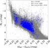 |
Fig. 1 Selecting a MS subsample of the EB catalogue. In gray: all Mowlavi et al. (2023) catalogue sources with ϖ/σϖ > 10, that have extinction parameters. In blue: 3404 sources with vbroad, for which vbroad / σvbroad > 2; the black line delineates the upper boundary of the main sequence – 124 sources are below the line. The black line is defined by the vertices: (−0.5, −2.5), (0.68, 1.2), (0.99, 3.68), (1.5, 5.28). |
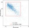 |
Fig. 2 vbroad vs. period for the MS eclipsing binary population of Fig 1, limited by vbroad >10 km/s and period ∈ [0.2, 10] days. The red square marks our analysis region (2082 sources). |
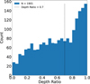 |
Fig. 3 Depth ratio histogram showing the 0.7 threshold applied to select 1050 systems with faint secondaries for further analysis. |
3 Analysis
We developed a tailored Markov chain Monte Carlo (MCMC) algorithm, similar to the one developed by Bashi et al. (2023), that searches for a probability density function ℱPDF that best describes the distribution of the points within the 2D region bounded by the red lines in Fig. 2. The algorithm fits the data with a 2D Gaussian function, which is rotated relative to the diagram axes. A full description of the algorithm is provided in Appendix A.
The results are presented in Fig. 4, which plots vbroad against period on a logarithmic scale. The best-fit parameters of the model are listed in Table B.1. The slope of the 2D Gaussian function is −0.948 ± 0.026. This linear trend, measured in log space, lies within 2σ of −1, consistent with synchronous rotation (Eq. (2)).
Following Eq. (1), while assuming that the short-period EBs are synchronised and aligned, we used the Gaia-derived radii and the EB period to estimate the expected rotational velocity of the primary star, denoted vrot. We then constructed a histogram of the ratio vbroad/vrot, shown in Fig. 5. The median value of the distribution is 0.87, indicating that vbroad is broadly consistent with vrot, though it exhibits a systematic lower offset of approximately ~10%.
Summary of the filtering process.
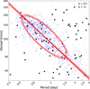 |
Fig. 4 Rotated 2D Gaussian representing the distribution of EBs in the (vbroad, period) plane. Line equation: log V = A log P + B, where A = −0.948 ± 0.026 and B = 1.952 ± 0.005. Black squares mark systems with |e cos ω| > 0.1, which are not fitted by the algorithm. The plot shows 100 parameter sets sampled from the MCMC chains after convergence. The red lines represent the Gaussian’s major-axis orientation, and the red ellipses show the distribution 3σ region. A full derivation is provided in Appendix B. |
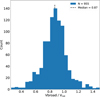 |
Fig. 5 vbroad/vrot for the synchronised binaries. The sample is limited to sources with vbroad/vrot in the range of [0.25, 1.5] for visual clarity. The black vertical line marks the median of the sample. |
4 Discussion
The analysis of the Gaia vbroad derived for a sample of 977 short-period EBs yielded two results.
The vbroad values are inversely proportional to the orbital period of the EBs.
-
Assuming the binaries of the sample are synchronised and aligned, the expected equatorial velocities of their primaries are, up to about 10%, similar to their derived vbroad.
These results suggest two things:
The short-period binaries are synchronised and aligned.
The derived vbroad represents the actual stellar equatorial velocity, with a systematic offset of ~10% lower.
Several studies have investigated the accuracy and robustness of deriving the stellar rotation velocity from spectral line broadening. For example, Royer et al. (2002a,b) conducted a large study of B8–F2-type stars across the southern and the northern skies. They reported that their V sin i measurements were systematically ~10% higher than those reported by Slettebak et al. (1975) (see also Slettebak 1955), probably due to the presence of binaries in the sample used by the early study. In contrast, our analysis compared the spectroscopically derived stellar rotation with those derived from the orbital periods obtained by photometry of EBs (see below Levato 1976; Lennon et al. 2024).
The approximately 10% lower vbroad we found may result from several factors. It could be the result of the inclination of the stellar rotational axis. However, we expect this factor to be small, as the systems are eclipsing, so their orbital inclinations are close to 90°, and we expect our systems to be aligned.
Another contributing factor could be an overestimation of the primary stellar radius due to the luminosity of the secondary component. Nevertheless, this is unlikely to fully explain the discrepancy, as we deliberately selected binaries with relatively faint secondaries, most of which contribute much less than ~20% of the total system luminosity. Such a small contribution would be insufficient to account for the ~10% increase in stellar radius (and, consequently, equatorial velocity) required to explain the observed discrepancy.
Therefore, the systematic offset may be attributed to residual biases in the analysis or underestimation of other line-broadening mechanisms.
Apart from the 10% systematic shift, the Gaia vbroad catalogue, and the catalogues of V sin i from other large spectroscopic surveys, such as GALAH (Buder et al. 2021) and APOGEE (Jönsson et al. 2020), can be used to estimate the stellar rotation period of large samples, albeit with lower accuracy due to their reliance on knowledge of stellar radius and inclination.
Observational evidence for synchronisation and alignment of samples of short-period binaries is crucial to our understanding of the long-term tidal interaction acting in close binaries (e.g., Hut 1981; Zahn 1989; Zahn & Bouchet 1989). In particular, the period limits between synchronised and non-synchronised binaries (e.g., Mathieu & Mazeh 1988) and their dependence on spectral type (e.g., Giuricin et al. 1984; Khaliullin & Khaliullina 2010) and mass ratio are essential. Unfortunately, the present Gaia EB catalogue is limited to short-period binaries, and the evidence for synchronisation of binaries with periods shorter than three days could be expected. However, the next Gaia data release, DR4, which will incorporate 66 months of observations compared to the 34 months included in DR3, will have longer-period EBs, enabling further study of tidal interaction.
Acknowledgements
We are deeply grateful to the referee, Dr. Nami Mowlavi, for his thorough review of the manuscript and for his insightful comments and suggestions, which greatly enhanced the clarity, structure, and scientific rigour of this work. His expertise and attention to detail were particularly valuable in refining the selection process to achieve more robust results. We deeply appreciate the time and effort he dedicated to the review process. We are also grateful to the Gaia CU6 and CU7 teams for releasing the vbroad and EB catalogues, which enabled this study through their extensive, high-quality data. TM is grateful for the support of Israel Ministry of Science Grant no. 3-18140. This work has made use of data from the European Space Agency (ESA) mission Gaia (https://www.cosmos.esa.int/gaia), processed by the Gaia Data Processing and Analysis Consortium (DPAC, https://www.cosmos.esa.int/web/gaia/dpac/consortium). Funding for the DPAC has been provided by national institutions, in particular those participating in the Gaia Multilateral Agreement.
References
- Aigrain, S., Llama, J., Ceillier, T., et al. 2015, MNRAS, 450, 3211 [Google Scholar]
- Bashi, D., Mazeh, T., & Faigler, S. 2023, MNRAS, 522, 1184 [Google Scholar]
- Breton, S. N., Santos, A. R. G., Bugnet, L., et al. 2021, A&A, 647, A125 [EDP Sciences] [Google Scholar]
- Buder, S., Sharma, S., Kos, J., et al. 2021, MNRAS, 506, 150 [NASA ADS] [CrossRef] [Google Scholar]
- Cropper, M., Katz, D., Sartoretti, P., et al. 2018, A&A, 616, A5 [NASA ADS] [CrossRef] [EDP Sciences] [Google Scholar]
- Frémat, Y., Royer, F., Marchal, O., et al. 2023, A&A, 674, A8 [NASA ADS] [CrossRef] [EDP Sciences] [Google Scholar]
- Gaia Collaboration (Prusti, T., et al.) 2016, A&A, 595, A1 [NASA ADS] [CrossRef] [EDP Sciences] [Google Scholar]
- Giuricin, G., Mardirossian, F., & Mezzetti, M. 1984, A&A, 131, 152 [Google Scholar]
- Hadad, E., Mazeh, T., Faigler, S., & Brown, A. G. A. 2025, A&A, 693, A214 [NASA ADS] [CrossRef] [EDP Sciences] [Google Scholar]
- Hut, P. 1981, A&A, 99, 126 [NASA ADS] [Google Scholar]
- Jönsson, H., Holtzman, J. A., Allende Prieto, C., et al. 2020, AJ, 160, 120 [Google Scholar]
- Khaliullin, K. F., & Khaliullina, A. I. 2010, MNRAS, 401, 257 [NASA ADS] [CrossRef] [Google Scholar]
- Lennon, D. J., Dufton, P. L., Villaseñor, J. I., et al. 2024, A&A, 688, A141 [NASA ADS] [CrossRef] [EDP Sciences] [Google Scholar]
- Levato, H. 1976, ApJ, 203, 680 [NASA ADS] [CrossRef] [Google Scholar]
- Lurie, J. C., Vyhmeister, K., Hawley, S. L., et al. 2017, AJ, 154, 250 [Google Scholar]
- Mathieu, R. D., & Mazeh, T. 1988, ApJ, 326, 256 [NASA ADS] [CrossRef] [Google Scholar]
- McQuillan, A., Aigrain, S., & Mazeh, T. 2013a, MNRAS, 432, 1203 [Google Scholar]
- McQuillan, A., Mazeh, T., & Aigrain, S. 2013b, ApJ, 775, L11 [Google Scholar]
- McQuillan, A., Mazeh, T., & Aigrain, S. 2014, ApJS, 211, 24 [Google Scholar]
- Mowlavi, N., Holl, B., Lecoeur-Taïbi, I., et al. 2023, A&A, 674, A16 [NASA ADS] [CrossRef] [EDP Sciences] [Google Scholar]
- Royer, F., Gerbaldi, M., Faraggiana, R., & Gómez, A. E. 2002a, A&A, 381, 105 [NASA ADS] [CrossRef] [EDP Sciences] [Google Scholar]
- Royer, F., Grenier, S., Baylac, M. O., Gómez, A. E., & Zorec, J. 2002b, A&A, 393, 897 [NASA ADS] [CrossRef] [EDP Sciences] [Google Scholar]
- Sartoretti, P., Katz, D., Cropper, M., et al. 2018, A&A, 616, A6 [NASA ADS] [CrossRef] [EDP Sciences] [Google Scholar]
- Slettebak, A. 1955, ApJ, 121, 653 [NASA ADS] [CrossRef] [Google Scholar]
- Slettebak, A., Collins, II, G. W., Boyce, P. B., White, N. M., & Parkinson, T. D. 1975, ApJS, 29, 137 [NASA ADS] [CrossRef] [Google Scholar]
- Steinmetz, M., Guiglion, G., McMillan, P. J., et al. 2020, AJ, 160, 83 [NASA ADS] [CrossRef] [Google Scholar]
- Xiang, M., Rix, H.-W., Ting, Y.-S., et al. 2022, A&A, 662, A66 [NASA ADS] [CrossRef] [EDP Sciences] [Google Scholar]
- Zahn, J. P. 1989, A&A, 220, 112 [Google Scholar]
- Zahn, J. P., & Bouchet, L. 1989, A&A, 223, 112 [NASA ADS] [Google Scholar]
Appendix
For each parameter set of the distribution ℱPDF—η, we derive the likelihood of N-binaries sample, as
![Mathematical equation: $\[\mathcal{L}=\prod_{i=1}^N \mathcal{F}_{\mathrm{PDF}}\left(\operatorname{vbroad}_i, \text { period }_i; \eta\right).\]$](/articles/aa/full_html/2025/09/aa55567-25/aa55567-25-eq4.png) (A.1)
(A.1)
where vbroadi and periodi are the vbroad and period of the i-th binary, given in km/s and days, respectively. We then find the parameter set η that maximises the likelihood of the sample.
The model function consists of a two-dimensional Gaussian combined with a uniform background density. It is characterised by the Gaussian centre coordinates (log p0, log v0): its angle, clockwise from the x-axis, θ; the standard deviations (in log space): σx, σy, and the peak density at the centre, D. The Gaussian is added to a rectangle with constant background density D. Therefore, given a set of parameters η, each point (vbroadi, periodi) is assigned a probability of
![Mathematical equation: $\[\mathcal{F}_{\mathrm{PDF}}\left(ubroad_i, period_i; \eta\right)=D e^{-\left(a P^2+b P V+c V^2\right)}+C,\]$](/articles/aa/full_html/2025/09/aa55567-25/aa55567-25-eq5.png) (A.2)
(A.2)
where
![Mathematical equation: $\[\begin{aligned}& P=\log \text { period}_i-\log~ \mathrm{p}_0, \\& V=\log \text { vbroad}_i-\log~ \mathrm{v}_0,\end{aligned}\]$](/articles/aa/full_html/2025/09/aa55567-25/aa55567-25-eq6.png)
and the a, b and c coefficients are
![Mathematical equation: $\[\begin{array}{r}a=\frac{\cos ^2 \theta}{2 \sigma_x^2}+\frac{\sin ^2 \theta}{2 \sigma_y^2} \\b=-\sin~ 2 \theta(\frac{1}{4 \sigma_x^2}-\frac{1}{4 \sigma_y^2}), \\c=\frac{\sin ^2 \theta}{2 \sigma_x^2}+\frac{\cos ^2 \theta}{2 \sigma_y^2}.\end{array}\]$](/articles/aa/full_html/2025/09/aa55567-25/aa55567-25-eq7.png) (A.3)
(A.3)
The domain area in log space is 1, so C is derived from the ℱPDF normalisation
![Mathematical equation: $\[D 2 \pi \sigma_x \sigma_y+C=1.\]$](/articles/aa/full_html/2025/09/aa55567-25/aa55567-25-eq8.png) (A.4)
(A.4)
Appendix
For a given parameter set η, a red line in Fig. 4 is calculated as
![Mathematical equation: $\[y=A x+B,\]$](/articles/aa/full_html/2025/09/aa55567-25/aa55567-25-eq9.png) (B.1)
(B.1)
for
![Mathematical equation: $\[A=-\tan~ \theta,\]$](/articles/aa/full_html/2025/09/aa55567-25/aa55567-25-eq10.png) (B.2)
(B.2)
and
![Mathematical equation: $\[B=\log~ \mathrm{v}_0+\tan~ \theta ~\log~ \mathrm{p}_0.\]$](/articles/aa/full_html/2025/09/aa55567-25/aa55567-25-eq11.png) (B.3)
(B.3)
The red ellipse’s left and right focal points are
![Mathematical equation: $\[\left(x_L, y_L\right)=\left(\log~ \mathrm{p}_0-d ~\cos~ \theta, ~\log~ \mathrm{v}_0+d ~\sin~ \theta\right),\]$](/articles/aa/full_html/2025/09/aa55567-25/aa55567-25-eq12.png) (B.4)
(B.4)
![Mathematical equation: $\[\left(x_R, y_R\right)=\left(\log~ \mathrm{p}_0+d ~\cos~ \theta, ~\log~ \mathrm{v}_0-d ~\sin~ \theta\right),\]$](/articles/aa/full_html/2025/09/aa55567-25/aa55567-25-eq13.png) (B.5)
(B.5)
for
![Mathematical equation: $\[d=\sqrt{\left|\left(3 \sigma_x\right)^2-\left(3 \sigma_y\right)^2\right|}.\]$](/articles/aa/full_html/2025/09/aa55567-25/aa55567-25-eq14.png) (B.6)
(B.6)
Then, the ellipse is the set of points (x′, y′) which satisfies:
![Mathematical equation: $\[\sqrt{\left(x^{\prime}-x_L\right)+\left(y^{\prime}-y_L\right)}+\sqrt{\left(x^{\prime}-x_R\right)+\left(y^{\prime}-y_R\right)}=2 max \left(3 \sigma_x, 3 \sigma_y\right).\]$](/articles/aa/full_html/2025/09/aa55567-25/aa55567-25-eq15.png) (B.7)
(B.7)
All Tables
All Figures
|
Fig. 1 Selecting a MS subsample of the EB catalogue. In gray: all Mowlavi et al. (2023) catalogue sources with ϖ/σϖ > 10, that have extinction parameters. In blue: 3404 sources with vbroad, for which vbroad / σvbroad > 2; the black line delineates the upper boundary of the main sequence – 124 sources are below the line. The black line is defined by the vertices: (−0.5, −2.5), (0.68, 1.2), (0.99, 3.68), (1.5, 5.28). |
| In the text | |
|
Fig. 2 vbroad vs. period for the MS eclipsing binary population of Fig 1, limited by vbroad >10 km/s and period ∈ [0.2, 10] days. The red square marks our analysis region (2082 sources). |
| In the text | |
|
Fig. 3 Depth ratio histogram showing the 0.7 threshold applied to select 1050 systems with faint secondaries for further analysis. |
| In the text | |
|
Fig. 4 Rotated 2D Gaussian representing the distribution of EBs in the (vbroad, period) plane. Line equation: log V = A log P + B, where A = −0.948 ± 0.026 and B = 1.952 ± 0.005. Black squares mark systems with |e cos ω| > 0.1, which are not fitted by the algorithm. The plot shows 100 parameter sets sampled from the MCMC chains after convergence. The red lines represent the Gaussian’s major-axis orientation, and the red ellipses show the distribution 3σ region. A full derivation is provided in Appendix B. |
| In the text | |
|
Fig. 5 vbroad/vrot for the synchronised binaries. The sample is limited to sources with vbroad/vrot in the range of [0.25, 1.5] for visual clarity. The black vertical line marks the median of the sample. |
| In the text | |
Current usage metrics show cumulative count of Article Views (full-text article views including HTML views, PDF and ePub downloads, according to the available data) and Abstracts Views on Vision4Press platform.
Data correspond to usage on the plateform after 2015. The current usage metrics is available 48-96 hours after online publication and is updated daily on week days.
Initial download of the metrics may take a while.