© The Authors 2025

1 Introduction

The magnetic field plays a crucial role in the high-mass star formation process, primarily because it can suppress the fragmentation process and transport angular momentum, keeping the matter close to the central object, where it can be accreted (e.g., Price & Bate 2007; Beuther et al. 2018; Krumholz & Federrath 2019). Observations at high angular resolution of maser emission lines from hydroxyl (OH), water (H₂ O), or methanol (CH₃OH) molecules are the best way to study the kinematics of gas in high-mass young stellar objects (HMYSOs; e.g., Moscadelli et al. 2011; Etoka et al. 2012; Bartkiewicz et al. 2016), whereas studying their polarized emission allows us to estimate the morphology and strength of magnetic fields (e.g., Bartkiewicz et al. 2005; Vlemmings et al. 2010; Surcis et al. 2011a). The pumping mechanism of the maser levels responsible for the CH₃OH maser emission at 6.7 GHz and of the excited OH (hereafter exOH) maser emission at 6.035 GHz is due to the infrared emission from warm dust heated by nearby HMYSOs. In addition, these maser emissions also share similar physical conditions such as temperature and density, making them possibly arise in the same volume of gas (Cragg et al. 2002). Therefore, if they arise in the same volume of gas, they must probe the same magnetic field; i.e., the same morphology and strength.

Hydroxyl (OH) is a paramagnetic molecule; i.e., it strongly interacts with an external magnetic field. This implies that the Zeeman splitting of its maser lines, for typical field strengths in massive star-forming regions, is larger than their linewidths. In other words, the frequency difference between the left- and right-handed circular polarized emissions (LHCP and RHCP), which correspond to the shifted σ components produced by the Zeeman effect, is easily measurable. Furthermore, the Landé g-factor and, consequently, the Zeeman splitting coefficient (α_Z) are known for many of the OH maser transitions (Davies 1974; Baudry et al. 1997), making the estimation of the magnetic field strength straightforward. Unlike OH, the CH₃OH molecule is non-paramagnetic; consequently, the Zeeman splitting of its maser lines is smaller than that of the maser linewidths, making the estimation of the magnetic field strength challenging but feasible (e.g., Vlemmings et al. 2010, 2011). It is important to note that in this case, the Zeeman splitting is not directly measured, but it must be estimated either by modeling the circularly polarized emission of the masers or by using a cross-correlation method (e.g., Modjaz et al. 2005; Vlemmings 2008; Vlemmings et al. 2010). In addition, all the CH₃OH masers show a very complex hyperfine structure (Lankhaar et al. 2016). For instance, eight hyperfine transitions can contribute to the maser emission at 6.7 GHz, and each one has its own Zeeman splitting coefficient (Lankhaar et al. 2018). At the moment, the dominant hyperfine transition for all of the CH₃OH masers is unknown, which prevents the estimation of the magnetic field strength from their Zeeman splitting estimates. Nevertheless, in the case of the 6.7 GHz CH₃OH maser emission the hyperfine transition F = 3 → 4 has been assumed to be the preferred one (e.g., Lankhaar et al. 2018; Surcis et al. 2022), although Dall'Olio et al. (2020) suggested that the dominant hyperfine transition might also be either F=6 → 7 A or F=7 → 8. However, the uncertainty on which is the dominating hyperfine transition renders the Zeeman splitting estimates made so far toward a large sample of HMYSOs almost worthless (e.g., Surcis et al. 2022). Therefore, it is crucial to find an observational strategy that allows us to identify the dominating hyperfine transition of the 6.7 GHz CH₃OH maser emission. A potential good strategy is that of observing the 6.7 GHz CH₃OH and the 6.035 GHz ex-OH maser emissions simultaneously toward the same HMYSOs. Indeed, the two maser emissions are thought to arise in the same volume of gas (Cragg et al. 2002), and consequently they might probe the same magnetic field.

In this paper, we present the comparison between the magnetic field strength and the Zeeman splitting as measured and estimated from the circularly polarized emission of the well-known 6.035 GHz ex-OH and of the 6.7 GHz CH₃OH maser emissions, respectively, with the aim of identifying the dominating hyperfine transition of the latter. The polarized maser emissions have been observed with the European VLBI Network (EVN) near two well-known HMYSOs: G69.540–0.976 (ON 1) and G81.871+0.781 (W75N). We selected these two sources according to recent single-dish (Szymczak et al. 2018, 2020) and interferometric results of a larger sample (Kobak et al. 2025). Kobak et al. (2025) observed the two HMYSOs with the e-MERLIN and showed that in both HMYSOs the CH₃OH and ex-OH maser features are very bright and strongly polarized; they shared the same local-standard-of-rest velocity (V_LSR) range, and their projected positions on the plane of the sky coincided. Unfortunately, e-MERLIN results cannot be used for our scientific purposes because the spatial resolution does not ensure the absence of maser line blending, which can severely affect the Zeeman splitting estimates of the CH₃OH maser. Furthermore, single-dish monitoring observations indicate that both maser emissions are variable on a timescale of one week to a few years (e.g., Szymczak et al. 2018, 2020). Below, we report a brief introduction of the two HMYSOs.

G69.540-0.976¹ (also known as Onsala 1, hereafter ON 1) is a high-mass star-forming region (HMSFR) at a parallactic distance of ${2.57}_{-0.27}^{+0.34}\mathrm{k}\mathrm{p}\mathrm{c}$ (Rygl et al. 2010). The archival ALMA data (2021.1.00311.S) show that the source hosts three cores of 1.3 mm dust continuum emission, the westernmost of which is an ultra-compact (UC) HII region that harbors an exciting type B0 star (Zheng et al. 1985; MacLeod et al. 1998; Argon et al. 2000; Nagayama et al. 2008; Hu et al. 2016) and is associated with 6.7 GHz CH₃OH and 6.035 GHz ex-OH masers (Nammahachak et al. 2006; Sugiyama et al. 2011; Surcis et al. 2022; Kobak et al. 2025). The other two cores, named WMC1 and WMC2, are associated with 22 GHz H₂O masers (Nagayama et al. 2008). Two molecular outflows were observed. The first one is traced by H¹³CO⁺ and SiO and it is oriented on the plane of the sky with a position angle (PA) of +44°, and the second one is traced by CO (PA=−69°; Kumar et al. 2004). It is still unclear which cores the two outflows are related to. The 6.7 GHz CH₃OH masers show a similar distribution to the 1.665 GHz OH masers, and both maser emissions are tracing an outward motion of the gas, likely suggesting the expansion of the UCHII region (Fish & Reid 2007; Sugiyama et al. 2011). Ground−state OH masers (1.665 GHz and 1.667 GHz) indicated magnetic field strength along the line of sight (B_∥) ranging from −0.9 mG to −5.1 mG (Fish et al. 2005), where a negative B_∥ indicates that the magnetic field is pointing toward the observer. Nammahachak et al. (2006) also measured a magnetic field of −0.4 mG and of −1 mG from two Zeeman pairs of 1.720 GHz OH masers. Recently, Kobak et al. (2025) measured magnetic fields in the −1.2 mG to −6.2 mG range from the 6.035 GHz ex-OH maser, which is consistent with those measured previously with the same ex-OH maser emission ($-1.1\mathrm{m}\mathrm{G}\le B_{\parallel }^{2007}\le -5.8\mathrm{m}\mathrm{G}$ and $-1.2\mathrm{m}\mathrm{G}\le B_{\parallel }^{2010}\le -12.1\mathrm{m}\mathrm{G}$; Green et al. 2007; Fish & Sjouwerman 2010). Green et al. (2007) also reported a magnetic field of −3.9 mG from the only Zeeman pair identified toward the OH maser emission at 6.031 GHz. In addition, they also estimated, using the cross-correlation method, the very first Zeeman splitting (ΔV_Z) of a 6.7 GHz CH₃OH maser – i.e., Δ V_Z = 0.9 ± 0.3 ms⁻¹ – using the MERLIN. More recently, Surcis et al. (2022) observed the 6.7 GHz CH₃OH maser emission with the EVN, and using the full radiative transfer method (FRTM) code they estimated two Zeeman splitting values of 14.5 ± 4.4 ms⁻¹ and 1.2 ± 0.2 m s⁻¹.

G81.871+0.781, known as W75N, is an HMSFR at a parallactic distance of 1.30 ± 0.07 kpc (Rygl et al. 2012). Several radio sources have been identified, among which the most interesting are VLA1 and VLA2 (e.g., Torrelles et al. 1997; Carrasco-González et al. 2010; Rodríguez-Kamenetzky et al. 2020). VLA1 is in an early stage of the photoionization, and it is driving a thermal radio jet (PA=+42°) whose morphology did not change over a period of 18 years (Rodríguez-Kamenetzky et al. 2020). VLA2 is a thermal, collimated, ionized wind surrounded by a dusty disk or envelope, and it varied its morphology between 1996 and 2014 from a compact, roundish source to an elongated source (PA=+65°; Carrasco-González et al. 2015). A large-scale CO outflow with PA of +66° was observed by Hunter et al. (1994). Different maser species are associated with VLA1 and VLA2: 6.7 GHz CH₃OH masers (e.g., Minier et al. 2001; Surcis et al. 2009), 1.665 GHz OH masers (e.g., Hutawarakorn et al. 2002; Fish et al. 2005, 2011), 6.035 GHz ex-OH masers (e.g., Kobak et al. 2025), and 22 GHz H₂O masers (e.g., Surcis et al. 2023). The CH₃OH and ex-OH masers are only detected toward VLA1; all the other maser species are detected toward both radio sources. A magnetic field strength between +3.7 and +8.1 mG, indicating that the magnetic field points away from the observer, was measured from the Zeeman effect of a 1.665 GHz OH maser line around VLA1 (Hutawarakorn et al. 2002; Fish et al. 2005), which is consistent with the values obtained from the Zeeman pair of 6.035 GHz ex-OH masers (+2.3 mG ≤ B_∥ ≤ +8.5 mG; Kobak et al. 2025). Surcis et al. (2009) reported Zeeman splitting estimates, determined via the cross-correlation method, toward three 6.7 GHz CH₃OH maser features, these are +0.53,+0.75, and +0.8 m s⁻¹. In addition, the magnetic field was measured along VLA1 from the 22 GHz H₂O maser emission at different epochs, indicating typical values in the range −764 mG ≤ B_∥ ≤ −676 mG (Surcis et al. 2023). The high values measured from the H₂O masers are the consequence of the high densities where these masers arise.

2 Observations and analysis

We observed ON 1 and W75N with nine antennas of the EVN (Jb, Wb, Ef, Mc, Nt, On, Tr, Ys, Ib) at 6035.092 MHz and 6668.519 MHz to detect the ex-OH and CH₃OH maser emissions (project code: EK052). To ensure quasi-simultaneous observations of the two maser species, we observed each source on two consecutive days: W75N on 29-30 May, 2023 and ON1 on 31 May-01 June, 2023. The observations were carried out with eight subbands of 4 MHz (∼ 100 km s⁻¹) each, both in phase-referencing (with cycles phase-calibrator – target of 2−3 min) and full-polarization mode, for a total observing time of 48 hours. The phase-referencing calibrators were J2003+3034 (at separation 1.7°) and J2048+4310(1.9°) for ON 1 and W75N, respectively. The data were correlated with the EVN software correlator (SFXC; Keimpema et al. 2015) in two correlation passes: a continuum pass for all eight subbands with 128 spectral channels; and a line pass for only the subband and the maser emission with 4096 spectral channels. The line pass allowed us to obtain a spectral resolution of ∼ 1 kHz (velocity resolution at both frequencies of ∼ 0.05 km s⁻¹) that is necessary to estimate the Zeeman splitting of the CH₃OH maser emission. All four polarization combinations (RR, LL, RL, and LR) were generated for all correlation passes.

The data were calibrated and imaged by using the Astronomical Image Processing Software package (AIPS, NRAO 2023) following the standard spectral polarimetric and phase-referencing procedures (e.g., Surcis et al. 2012, 2023). For all the datasets, we used the calibrator J2202+4216 (BL Lac) to calibrate the bandpass, the delay, the phase, the rates, and the D-terms. The calibration of the polarization angles was instead performed on the calibrator 3C286 (I ≈ 0.2 Jy beam⁻¹; linear polarization percentage P₁ ≈ 12%) for all but one dataset. We could not use 3C286 to calibrate the polarization angles of the CH₃OH masers in W75N due to a problem with the 3C286 data. Therefore, we decided to compare the calibrated polarization angle of J2202+4216 from the ON 1 dataset (PA=−13°.2 ± 2°.1), which was calibrated using 3C286, with that observed in the W75N dataset, and then applied the rotation to the linear polarization vectors of the CH₃OH masers in W75N. The uncertainty of this calibration is equal to 7°. We self-calibrated the brightest maser spot of each dataset and applied the solutions to the corresponding dataset. To determine the absolute positions of the maser spots, we performed the phase-referencing calibration between the calibrator and the channel of the brightest maser spot for each dataset. The uncertainties of the absolute positions of the reference brightest maser spot were estimated following Kobak et al. (2025). Afterward, we imaged the four I, Q, U, and V Stokes cubes (the latter only for the CH₃OH masers) and the RR and LL cubes. The Q and U cubes were combined to produce cubes of linearly polarized intensity ($POLI=\sqrt{Q^2+U^2}$) and polarization angle (POLA =0.5 × atan(U/Q)). The root mean square (rms) noise and the beam size for each imaged cube is reported in Table 1.

The identification of CH₃OH and ex-OH maser features was done as described in Surcis et al. (2011a). In particular, the CH₃OH maser features were searched in the I Stokes cube and the ex-OH maser features in the I, RR, and LL cubes. A maser feature is identified when at least three maser spots in consecutive spectral channels are spatially coincident within the beam; therefore, the uncertainty in the identification process is equal to half of the beam. We measured the mean linear polarization percentage (P₁) and the mean linear polarization angle (χ) for each identified CH₃OH maser feature, considering only the consecutive channels (at least two) across the total intensity spectrum for which the polarized intensity is greater than or equal to 4 σ_POLI.

The linearly polarized CH₃OH maser features were then analyzed by using the full radiative transfer method (FRTM) code described in Surcis et al. (2019). With this code, we modeled the total intensity (I) and the POLI spectra. The outputs of the FRTM code are the emerging brightness temperature (T_b ΔΩ, where Ω is the maser beaming solid angle), the intrinsic maser linewidth (ΔV_i), and the angle between the magnetic field and the maser propagation direction (θ). If θ is greater than the Van Vleck angle (θ_crit ≈ 55°), the magnetic field is perpendicular to the linear polarization angle; otherwise, it is parallel (Goldreich et al. 1973). We note that the FRTM code only works properly for unsaturated masers (e.g., Vlemmings et al. 2010; Surcis et al. 2011b). This implies that if the code is performed on a saturated maser, the Δ V_i and T_b Δ Ω outputs are overestimated and underestimated, respectively (e.g., Surcis et al. 2011b). Furthermore, the saturation of the masers introduces a more complex dependence of the magnetic field with θ (Nedoluha & Watson 1992), and consequently the FRTM code provides an overestimate of θ for these masers, which could also reach values of 90°. A 6.7 GHz CH₃OH maser feature can be considered partially saturated if T_b Δ Ω > 2.6 × 10⁹ K sr. However, the orientation of the magnetic field with respect to the linear polarization vectors is not affected by the saturation of the masers (Surcis et al. 2011b). Finally, the best estimates of T_b Δ Ω and Δ V_i were used to produce I and V models with the FRTM code that were used to fit the circularly polarized CH₃OH maser feature. A CH₃OH maser feature is considered circularly polarized if the measured V peak intensity is both >3 σ_V and >3 σ_s.–n., where σ_s.–n. is the self-noise produced by the maser feature in its channels and becomes important when the power contributed by the astronomical maser is a significant portion of the total received power (Sault 2012). From the best I and V models, we were able to estimate the circular polarization percentage (P_V) and Δ V_Z of the CH₃OH maser features. We note that the FRTM code is able to estimate Δ V_Z even if these maser features are partially saturated. These estimates were also made by using the cross-correlation method between the RR and LL spectra.

For each ex-OH maser feature identified in I cubes, we determined its LL and RR counterparts (>3 σ_LL and >3 σ_RR) based on their positions on the plane of the sky, to pair them in a so-called Zeeman pair (shifted σ components), similarly to what was done in Kobak et al. (2025). The LL and RR features were fit with a Gaussian profile that provided the peak intensity and velocity of the maser features. From the velocity difference between the LL and RR peaks of a Zeeman pair, we measured Δ V_Z, and from their and corresponding I intensity peaks we measured P_V. Knowing that the Zeeman coefficient for the ex-OH at 6.035 GHz is ${\alpha }_{\mathrm{Z}}^{\mathrm{e}\mathrm{x}-\mathrm{O}\mathrm{H}}=0.056{\mathrm{m}\mathrm{s}}^{-1}{\mathrm{G}}^{-1}$ (Davies 1974; Baudry et al. 1997), $B=\mathrm{\Delta }{V}_{\mathrm{Z}}/{\alpha }_{\mathrm{Z}}^{\text{ex-OH}}$, which is equal to B_∥ if the unshifted π component due to the Zeeman effect is negligible. We measured P₁ and χ for each identified ex-OH maser feature, similarly to what we did for the CH₃OH maser features, but in this case we considered the channels with polarized intensity greater than or equal to 3σ_POLI. For OH masers, and consequently for ex-OH maser emission, the orientation of the magnetic field on the plane of the sky, Φ_B, is perpendicular to the linear polarization vector for σ components and parallel to it for the π component. As observations have shown in the past, the emission of σ components usually dominates over the π component, implying that the magnetic field is perpendicular to the linear polarization vector (e.g., Gray et al. 2003; Green et al. 2015). In particular, in about 16% of the observed cases the π component of ex-OH masers is detected, and only in ∼1% is no intrinsic π emission present, suggesting that in all the other cases some unidentified suppression mechanism of the linearly polarized emission (π component) must be at play (e.g., Green et al. 2015). Moreover, the magnetic field is only parallel to the linear polarization vector when P₁ ≥ 71%. Indeed, only in this case does the unshifted π component contribute the most to P₁ (Fish & Reid 2006). According to our findings (see Sect. 3), we can assume that the π component (< 3σ) is negligible and, therefore, that the magnetic field is always perpendicular to the linear polarization vectors and we can assume B ≈ B_∥from our Zeeman splitting measurements.

3 Results

We detected the 6.7 GHz CH₃OH and 6.035 GHz ex-OH maser emissions toward both ON 1 and W75N. The distributions of the identified maser features are shown in Figure 1, and their parameters are reported in Tables A.1–A.4. Their total spectra are shown in Figures B.1 and B.2. Below, we briefly summarize our results.

3.1 G69.540-0.976 (ON 1)

We detected 11 CH₃OH (named G69.M01-G69.M11) and 24 ex-OH (named G69.E01-G69.E24) maser features toward ON 1. Both maser species are spatially distributed in two main groups: one blue-shifted and located in the north of the UCHII region and one red-shifted and located in the south (see Figure 1). Their distribution and V_LSR are very similar to those reported previously in Kobak et al. (2025).

Only the brightest CH₃OH maser feature (G69.M04, I = 11 Jy beam⁻¹ and V_LSR = 14.68 km s⁻¹) shows polarized emission; in particular, we measured a linear polarization percentage of P₁=0.4% and a circular polarization percentage of P_V=0.6%, which is identical to what was measured in 2015 (Surcis et al. 2022). Although P₁ is one third lower than previously measured, the linear polarization angle, χ=−58° ± 6°, is similar (χ²⁰¹⁵=−34° ± 9°; Surcis et al. 2022). We were able to properly fit G69.M04 with the FRTM code. The hyperfine transition F=3 → 4 was assumed as the preferred one, which provided a value of $\theta =+{75}_{-37}^{\circ +13}$, indicating that the orientation of the magnetic field on the plane of the sky is more likely (with a probability of 66% that θ > 55°) perpendicular to the linear polarization vector (see Sect. 2). We note that the FRTM code would provide similar output values, within the errors, for T_b Δ Ω, Δ V_i, and θ if we assume any other hyperfine transition, this is basically due to the size of our uncertainties. By modeling its V spectrum (see Figure 2) and by cross-correlating the RR and LL spectra, we estimated a Zeeman splitting of 3.2 m s⁻¹.

We measured linearly polarized emission toward five exOH maser features (3.7% ≤ P₁ ≤ 16%), with a mean value equal to 7.8% ± 4.95% and a median value equal to 6.2%. The linear polarization vectors have position angles ranging from −93° to −42°, with mean and median values of −68° ± 24° and −75°, respectively. We measured circularly polarized emission toward all but one (G69.E13) of the ex-OH maser features, but only for 12 of them were we able to identify Zeeman pairs (for them P_V ≥ 77%). This implies that the shifted σ components dominate over the unshifted π component, and consequently the magnetic field is perpendicular to the linear polarization vectors (see Sect. 2). Therefore, Φ_B is oriented northeast-southwest $({\mathrm{\Phi }}_{\mathrm{B}}^{\mathrm{e}\mathrm{x}-\mathrm{O}\mathrm{H}}=+{22}^{\circ }\pm {24}^{\circ })$. Furthermore, we measured the magnetic field along the line of sight for four blueshifted (−12.67 mG ≤ B_∥ ≤−5.98 mG) and eight red-shifted (−6.37 mG ≤ B_∥ ≤−1.35 mG) ex-OH maser features.

3.2 G81.871+0.781 (W75N)

We identified almost five times the number of 6.7 GHz CH₃OH maser features toward W75N than was previously done by Surcis et al. (2009); i.e., 47 (named here W75.M01-W75N.M47) versus 10. That is due to the high sensitivity of our EVN observations compared to those performed in 2008; indeed, Surcis et al. (2009) reported maser features with peak intensities of 2 Jy beam ⁻¹ ≤ I ≤ 95.4 Jy beam ⁻¹, while we have maser features with 0.03 Jy beam⁻¹ ≤ I ≤ 25.9 Jy beam⁻¹ (see Table A.3). The maser distribution and the V_LSR range of the CH₃OH maser features are identical to those of 2008; i.e., +3.37 km s⁻¹ ≤ V_LSR ≤ +9.51 km s⁻¹ (see Fig. 1). We also identified five 6.035 GHz ex-OH maser features (named W75N.E01-W75N.E05) with +6.87 km s⁻¹ ≤ V_LSR ≤+8.13 km s⁻¹ that spatially overlap on the plane of the sky with the CH₃OH maser features that have a similar velocity range (see Fig. 1 for a direct comparison). All maser features are associated with the radio continuum source VLA 1.

We detected linearly polarized emission from 16 CH₃OH maser features that show extremely high P₁, for all but one ($P_1^{\text{W75N.M34}}=3.3\mathrm{\%}$), ranging from 6.8 to 13.4%. For comparison, this was $0.9\mathrm{\%}\le P_1^{2008}\le 4.5\mathrm{\%}$ in 2008 (Surcis et al. 2009). The linear polarization vectors have position angles between −41° and +5°, with a mean value of −14° ± 7°(χ²⁰⁰⁸=. −17° ± 10°, Surcis et al. 2009). The high percentage of linear polarization suggests either that all the maser features might be saturated and/or that one hyperfine transition is preferred (Dall'Olio et al. 2020). However, we report the outputs (Δ V_i, T_b Δ Ω, and θ) of the FRTM code, where we assumed the hyperfine transition F=3 → 4 as the preferred one, in Table A.3. The estimated θ values are all greater than 55° (see Section 2); therefore, the magnetic field is perpendicular to the linear polarization vectors of the CH₃OH maser features. Actually, all the θ values are equal to 90°, suggesting that all the maser features might be partially saturated, and therefore the θ values might be overestimated but still greater than θ_crit ≈ 55° (see Sect. 2). We detected circular polarization toward three CH₃OH maser features $(P_{\mathrm{V}}^{\mathrm{W}75\mathrm{N}.\mathrm{M}21}=0.9\mathrm{\%},P_{\mathrm{V}}^{\mathrm{W}75\mathrm{N}.\mathrm{M}29}=1.4\mathrm{\%}$., and $P_{\mathrm{V}}^{\mathrm{W}75\mathrm{N}.\mathrm{M}43}1.0\mathrm{\%}=$). Actually, the detection of $P_{\mathrm{V}}^{\mathrm{W}75\mathrm{N}.\mathrm{M}43}$ must be considered as tentative since the V Stokes emission is about 2 σ_s.−n. (see Fig. 2). From these features, we were able to estimate Zeeman splitting of $\mathrm{\Delta }{V}_{\mathrm{Z}}^{\mathrm{W}75\mathrm{N}.\mathrm{M}21}=+1.2\mathrm{m}{\mathrm{s}}^{-1},\mathrm{\Delta }{V}_{\mathrm{Z}}^{\mathrm{W}75\mathrm{N}.\mathrm{M}29}=+2.1\mathrm{m}{\mathrm{s}}^{-1}$, and $\mathrm{\Delta }{V}_{\mathrm{Z}}^{\mathrm{W}75\mathrm{N}.\mathrm{M}43}=+1.6\mathrm{m}{\mathrm{s}}^{-1}$ by modeling the V spectra. The cross-correlation method provided consistent values for W75N.M21 and W75N.M29, but no value was determined for W75N.M43. In 2008, three CH₃OH maser features showed P_V ≈ 0.5% and +0.5 m s⁻¹ ≤ Δ V_Z ≤+0.8 m s⁻¹ (Surcis et al. 2009).

We only measured linearly polarized emission toward the ex-OH maser feature W75N.E02, for which P₁=1.7% ± 0.6% and χ=−36° ± 11°, and circularly polarized emission for all the features (P_v ≥ 82%). The sky component of the magnetic field is then oriented on the plane of the sky with an angle of ${\mathrm{\Phi }}_{\mathrm{B}}^{ex-OH}=+{54}^{\circ }\pm {11}^{\circ }$. Furthermore, we identified five Zeeman pairs from which we measured magnetic field strength along the line of sight between +2.47 mG and +8.64 mG. These values are consistent with those obtained with the e-MERLIN observations – i.e., $+2.3\mathrm{m}\mathrm{G}\le B_{\parallel }^{\text{ex-}\mathrm{O}\mathrm{H},2025}\le +8.5\mathrm{m}\mathrm{G}-$ and reported in Kobak et al. (2025).

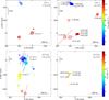Fig. 1 Distribution of 6.7 GHz CH3OH (left panels, circle symbols) and 6.035 GHz ex-OH (right panel, square symbols) maser features detected around ON 1 (top panels; $V_{\mathrm{L}\mathrm{S}\mathrm{R},\mathrm{s}\mathrm{y}\mathrm{s}}^{\mathrm{O}\mathrm{N}1}=+11.6\mathrm{k}\mathrm{m}{\mathrm{s}}^{-1}$; Bronfman et al. 1996) and W75N (bottom panels; $V_{\mathrm{L}\mathrm{S}\mathrm{R},\mathrm{s}\mathrm{y}\mathrm{s}}^{\mathrm{W}75\mathrm{N}}=+10.0\mathrm{k}\mathrm{m}{\mathrm{s}}^{-1}$; Shepherd et al. 2003). The size of the symbols is scaled logarithmically according to their peak intensity (see Tables A.1–A.4), while their colors indicate the VLSR (see Tables A.1–A.4). The reference positions are RA(J2000)=20h 10m09s.04272±0s.00007 and Dec(J2000)=+31° 31′ 34′′.9736 ± 0′.0009 for ON 1; and RA(J2000)=20h 38m 36.41744 ± 0.00008 and Dec(J2000)=+42° 37′ 35′′.1153 ± 0′.0011 for W75N. The measured linear polarization vectors with their scales, the estimated $\mathrm{\Delta }{V}_{\mathrm{Z}}^{{CH}_{3}OH}$, and the measured $B_{\parallel }^{ex-OH}$ are also reported.

4 Discussion

The strategy to identify the most favored hyperfine transition of the 6.7 GHz CH₃OH maser emission is based on the successful calculations of the Zeeman splitting of CH₃OH and ex-OH maser lines toward the same volume of gas. This can be done if we assume that the magnetic field probed by the two maser species is exactly the same and that its strength is constant within the volume of gas where the masers arise. Therefore, the first step is to determine if the two maser species are probing the same magnetic field (see Sect. 4.1) and then comparing the Zeeman splitting estimates (see Sect.4.2). In Sect.4.3, we compare the magnetic fields we measured with those obtained in the past.

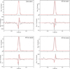Fig. 2 Total intensity (I, upper panel) and circularly polarized intensity (V, lower panel) spectra for the 6.7 GHz CH3OH maser features named G69.M04, W75N.M21, W75N.M29, and W75N.M43 (see Tables A.1, and A.3). The thick red lines are the best-fit models of I and V emissions obtained using the adapted FRTM code (see Sect. 2). The maser features were centered on zero velocity.

4.1 Magnetic field orientation in ON 1 and W75N

If the CH₃OH and ex-OH masers are probing the same magnetic field, we expect that the orientation on the plane of the sky of the magnetic field, as estimated from the linearly polarized emission of the two maser species, is consistent within the same source. We note that, although we assumed the unshifted π component of the polarized ex-OH maser features negligible according to our measurements (see Tables A.2 and A.4), the magnetic field must not be considered purely parallel to the line of sight. However, only the π component can be suppressed by some still-unknown mechanism (e.g., Green et al. 2015). Indeed, from the linear polarization of the σ components, we were able to estimate the orientation of the magnetic field on the plane of the sky, which would have been impossible in the case of a magnetic field purely oriented along the line of sight. Therefore, comparing the projected orientation of the magnetic field as estimated from the two maser emissions is still a good approximation.

We measured the magnetic field orientations of ${\mathrm{\Phi }}_{\mathrm{B}}^{{\mathrm{C}\mathrm{H}}_3\mathrm{O}\mathrm{H}}=+{32}^{\circ }\pm 6^{\circ }$ and $⟨{\mathrm{\Phi }}_{\mathrm{B}}^{\mathrm{e}\mathrm{x}-\mathrm{O}\mathrm{H}}⟩=+{22}^{\circ }\pm {24}^{\circ }$ in ON 1. These measurements agree within the uncertainties (see Fig.1). The magnetic field in ON1 is almost oriented along one of the outflows observed toward the region, particularly the one traced by H¹³CO⁺and SiO(PA=+44°). Also in the case of W75N the orientation of the magnetic field on the plane of the sky is consistent (see Fig. 1) between the one estimated from the polarized CH₃OH maser emission ($⟨{\mathrm{\Phi }}_{\mathrm{B}}^{{\mathrm{C}\mathrm{H}}_3\mathrm{O}\mathrm{H}}⟩=+{76}^{\circ }\pm 7^{\circ }$) and that from the ex-OH maser-polarized emission (${\mathrm{\Phi }}_{\mathrm{B}}^{\mathrm{e}\mathrm{x}-\mathrm{O}\mathrm{H}}=+{54}^{\circ }\pm {11}^{\circ }$). According to our findings, we can assume that the two maser species are likely probing the same magnetic field in each source.

4.2 Attempts to identify the favored hyperfine transition for the 6.7 GHz CH₃OH maser emission

Because the 6.7 GHz CH₃OH and 6.035 GHz ex-OH masers trace a very similar orientation of the magnetic field on the plane of the sky in both sources, we can measure the Zeeman splitting coefficient of the CH₃OH maser (${\alpha }_{\mathrm{Z}}^{C{H}_{3}OH}$) using the following relation: $${\alpha }_{\mathrm{Z}}^{{CH}_{3}OH}=\frac{\mathrm{\Delta }{V}_{\mathrm{Z}}^{{CH}_{3}OH}}{B_{\parallel }^{ex-OH}},$$(1)

where $\mathrm{\Delta }{V}_{\mathrm{Z}}^{{\mathrm{C}\mathrm{H}}_3\mathrm{O}\mathrm{H}}$ is the estimated Zeeman splitting of the CH₃OH maser and $B_{\parallel }^{ex-OH}$ is the magnetic field strength along the line of sight as measured from the ex-OH maser emission. We note that being able to use $B_{\parallel }^{ex-OH}$ rather than B^ex−OH reduces the sources of uncertainty. Indeed, from the estimation of $\mathrm{\Delta }{V}_{\mathrm{Z}}^{{CH}_{3}OH}$ it is only possible to measure $B_{\parallel }^{{\mathrm{C}\mathrm{H}}_3\mathrm{O}\mathrm{H}}$ (e.g., Vlemmings 2008) and not $B^{{CH}_{3}OH}=B_{\parallel }^{{CH}_{3}OH}/\cos \theta$, for which we would have introduced the large uncertainties in the estimation of θ. Our criteria to couple the ex-OH maser features with the CH₃OH maser features are, in order of importance, (1) the measurement of $B_{\parallel }^{ex-OH}$ and estimate of $\mathrm{\Delta }{V}_{\mathrm{Z}}^{{\mathrm{C}\mathrm{H}}_3\mathrm{O}\mathrm{H}}$; (2) the separation on the plane of the sky, the smaller the better; and (3) a similar V_LSR, the closer the better.

We estimated only one Zeeman splitting toward the 6.7 GHz CH₃OH maser features in ON 1, i.e., G69.M04 $(V_{\text{LSR}}^{\mathrm{G}69.\mathrm{M}04}=+14.68\mathrm{k}\mathrm{m}{\mathrm{s}}^{-1})$. We can couple it with G69.E06, which is the closest ex-OH maser feature (with a separation of d=184 mas, i.e. 470 au) with similar velocity ($V_{\text{LSR}}^{\mathrm{G}69.{}^{\mathrm{E}06}}=+15.19\mathrm{k}\mathrm{m}{\mathrm{s}}^{-1}$), from which we measured magnetic field strength along the line of sight; i.e., $B_{\parallel }^{\mathrm{G}69\cdot \mathrm{E}06}=-4.52\mathrm{m}\mathrm{G}$.

In the case of W75N, we estimated the Zeeman splitting toward three CH₃OH maser features: W75N.M21, W75N.M29, and W75N.M43 (tentative, see Sect.3.2). Unfortunately, only W75N.M43 $(V_{\text{LSR}}^{\text{W75N.M43}}=+7.40\mathrm{k}\mathrm{m}{\mathrm{s}}^{-1})$ is almost coincident with ex-OH maser features (W75N.E01 at d=48 mas and W75N.E02 at d=182 mas, i.e., 63 au and 240 au, respectively) with similar velocities($V_{\text{LSR}}^{\text{W75N.E01}}=+7.20\mathrm{k}\mathrm{m}{\mathrm{s}}^{-1}$ and $V_{\text{LSR}}^{\text{W75N.E02}}=+6.87\mathrm{k}\mathrm{m}{\mathrm{s}}^{-1}$), for which we measured $B_{\parallel }^{\text{ex-OH}}$. The other two – i.e., W75N.M21 ($V_{\text{LSR}}^{\text{W75N.M21}}=+4.64\mathrm{k}\mathrm{m}{\mathrm{s}}^{-1}$) and W75N.M29 $(V_{\text{LSR}}^{\text{W75N.M29}}=+4.11\mathrm{k}\mathrm{m}{\mathrm{s}}^{-1})$ – are much further from the closest ex-OH maser feature W75N.E02: 367 mas (480 au) and 417 mas (540 au), respectively.

We list the calculated ${\alpha }_{\mathrm{Z}}^{{\mathrm{C}\mathrm{H}}_3\mathrm{O}\mathrm{H}}$ values (see Eq. (1)) in Table 2 (Col. 5) for all the pairs of maser features (Col. 1) mentioned above. The other parameters reported in Table 2 are the maser features' separation (Col. 2); the estimated Zeeman splitting of CH₃OH 's maser emission (Col. 3); the magnetic field along the line of sight measured from the ex-OH maser features (Col.4). The ${\alpha }_{\mathrm{Z}}^{{\mathrm{C}\mathrm{H}}_3\mathrm{O}\mathrm{H}}$ obtained from Eq. (1) do not coincide with any of the Zeeman coefficients of the eight hyperfine transitions of the 6.7 GHz CH₃OH maser emission reported in the supplementary Table 3 of Lankhaar et al. (2018). This implies that the two maser emissions might not arise in the same volume of gas, or, in other words, that the gas density where they arise is slightly different. Indeed, this condition can still provide the same morphology of the magnetic field, but with a different strength.

To compare the number densities of the gas where the CH₃OH $\left(n_{{\mathrm{H}}_2}^{{\mathrm{C}\mathrm{H}}_3\mathrm{O}\mathrm{H}}\right)$ and ex-OH $\left(n_{{\mathrm{H}}_2}^{\text{ex-}\mathrm{O}\mathrm{H}}\right)$ maser emissions arise, we needed to determine the magnetic field strength ($B_{\parallel }^{{\mathrm{C}\mathrm{H}}_3\mathrm{O}\mathrm{H}}$ from the Zeeman splitting estimates of the 6.7 GHz CH₃OH maser emission. Indeed, following Crutcher & Kemball (2019) we know that

$$\eta \equiv \frac{n_{{\mathrm{H}}_2}^{\mathrm{e}\mathrm{x}-\mathrm{O}\mathrm{H}}}{n_{{\mathrm{H}}_2}^{{\mathrm{C}\mathrm{H}}_3\mathrm{O}\mathrm{H}}}={\left(\frac{\left|B_{\parallel }^{\mathrm{e}\mathrm{x}-\mathrm{O}\mathrm{H}}\right|}{\left|B_{\parallel }^{{\mathrm{C}\mathrm{H}}_3\mathrm{O}\mathrm{H}}\right|}\right)}^2.$$(2)

To estimate $B_{\parallel }^{{\mathrm{C}\mathrm{H}}_3\mathrm{O}\mathrm{H}}$, we can assume that one of the eight hyperfine transitions is more favored than the others. As suggested by Lankhaar et al. (2018), this might be F=3 → 4 (${\alpha }_{\mathrm{Z},3\to 4}^{{\mathrm{C}\mathrm{H}}_3\mathrm{O}\mathrm{H}}=-50.955\mathrm{m}{\mathrm{s}}^{-1}{\mathrm{G}}^{-1}$), because it shows the largest Einstein coefficient. Furthermore, it provides the lowest value of $B_{\parallel }^{{\mathrm{C}\mathrm{H}}_3\mathrm{O}\mathrm{H}}$ (Lankhaar et al. 2018). As expected (see Table 3), the $B_{\parallel }^{{\mathrm{C}\mathrm{H}}_3\mathrm{O}\mathrm{H}}$ values obtained assuming F=3 → 4 are larger than those obtained from the associated ex-OH maser features both in ON 1 and W75N. However, ON 1 $B_{\parallel }^{{\mathrm{C}\mathrm{H}}_3\mathrm{O}\mathrm{H}}$ and $B_{\parallel }^{\text{ex-}\mathrm{O}\mathrm{H}}$ have the same sign, while they are opposite in W75N for all the maser features. Moreover, while in ON 1 η is about 0.005, in W75N it is at least one order of magnitude larger. Therefore, we can suppose that F=3 → 4 might be the favored hyperfine transition in ON 1, but this is not the case in W75N. For W75N, we can thus assume that either $\mathrm{F}=6\to 7\mathrm{A}({\alpha }_{\mathrm{Z},6\to 7\mathrm{A}}^{{\mathrm{C}\mathrm{H}}_3\mathrm{O}\mathrm{H}}=+10.067\mathrm{m}{\mathrm{s}}^{-1}{\mathrm{G}}^{-1})$ or $\mathrm{F}=7\to 8({\alpha }_{\mathrm{Z},7\to 8}^{{\mathrm{C}\mathrm{H}}_3\mathrm{O}\mathrm{H}}=+21.176\mathrm{m}{\mathrm{s}}^{-1}{\mathrm{G}}^{-1})$ is the favored one. Indeed, Dall'Olio et al. (2020) suggested these as alternative dominant hyperfine transitions. The results are listed in Table 3. The sign of $B_{\parallel }^{{\mathrm{C}\mathrm{H}}_3\mathrm{O}\mathrm{H}}$ matches that of $B_{\parallel }^{\text{ex-}\mathrm{O}\mathrm{H}}$ for both hyperfine transitions, and also the η values are comparable to what we measure in ON 1. Nevertheless, it is not possible to identify which of them is the most favorable. Speculatively, we can state that the two maser emissions arise close to each other, with the 6.7 GHz CH₃OH maser features being closer to the HMYSO, where the gas density is about two orders of magnitude larger than that where the ex-OH maser features arise. This statement can be considered in agreement with the theoretical number-density ranges for the two maser emissions: ${10}^5{\mathrm{c}\mathrm{m}}^{-3}<n_{{\mathrm{H}}_2}^{{\mathrm{C}\mathrm{H}}_3\mathrm{O}\mathrm{H}}<{10}^9{\mathrm{c}\mathrm{m}}^{-3}$ and $3\times {10}^6{\mathrm{c}\mathrm{m}}^{-3}<n_{{\mathrm{H}}_2}^{\mathrm{e}\mathrm{x}-\mathrm{O}\mathrm{H}}<3\times {10}^8{\mathrm{c}\mathrm{m}}^{-3}$ (Cragg et al. 2002, 2005).

4.3 Comparison of magnetic fields over a long period of time

Both ON 1 and W75N were previously searched for polarized maser emissions at 6.035 GHz (ex-OH) and 6.7 GHz (CH₃OH) to probe their magnetic field morphology and strength. Below, we describe their changes over the years.

4.3.1 G69.540-0.976 (ON 1)

ON1 shows very stable magnetic field morphology over about 20 years. Indeed, Green et al. (2007) measured linear polarization vectors for two red-shifted 6.035 GHz ex-OH maser features (χ²⁰⁰⁷=−87.7° ± 2.0° and −42.5° ± 0.7°), corresponding to our features G69.E22 and G69.E24, and for one red-shifted 6.031 GHz ex-OH maser feature (χ²⁰⁰⁷=−43.1° ± 1.9°), corresponding to our G69.E03, which show the orientation on the plane of the sky to be identical, within the errors, to our measurements. However, we must note that Fish & Sjouwerman (2010) also reported three measurements of linear polarization vectors toward the 6.035 GHz ex-OH maser features. Two of them – their features K and Z (χ^K,2010 = +52°. and.χ^Z, 2010=−32°)− can be associated with our features G69.E22 and G69.E03, respectively. Although a direct comparison is difficult because no errors are reported by Fish & Sjouwerman (2010), taking into account our uncertainties, we have differences of −25° and −11°, respectively. It is important to emphasize that the linear polarization vectors measured by us toward the ex-OH maser features are all but one (G69.E03, with a difference of −12°) in perfect agreement with those measured with the e-MERLIN by Kobak et al. (2025). Therefore, for about 20 years the magnetic field, which is always perpendicular to the linear polarization vectors, has been constantly oriented southwest-northeast in the region where the red-shifted maser features arise. Besides the morphology of the magnetic field, we also find that B_∥ did not substantially vary over the same period of time. Green et al. (2007), Fish & Sjouwerman (2010), and Kobak et al. (2025) measured B_∥ toward five, eleven, and five maser features, respectively, with values in the ranges of $-5.8\mathrm{m}\mathrm{G}\le B_{\parallel }^{2007}\le -1.1\mathrm{m}\mathrm{G},-12.1\mathrm{m}\mathrm{G}\le B_{\parallel }^{2010}\le -1.3\mathrm{m}\mathrm{G}$, and $-6.2\mathrm{m}\mathrm{G}\le B_{\parallel }^{2025}\le -1.2\mathrm{m}\mathrm{G}$. By comparing these values with our measurements, we note differences of less than 25%, which might be due to a high-performance modern instrument, a real magnetic field variation, or both. It is interesting to note that the magnetic field strength measured from the Zeeman effect of ground-state OH maser emissions (1.665 and 1.667 GHz) covers a similar range of values: $-3.6\mathrm{m}\mathrm{G}\le B_{\parallel }^{\mathrm{O}\mathrm{H}}\le -0.8\mathrm{m}\mathrm{G}$ (Fish et al. 2005; Nammahachak et al. 2006).

We can compare the magnetic field morphology as probed by the 6.7 GHz CH₃OH masers over eight years. In 2015, Surcis et al. (2022) measured linear polarization vectors for two maser features: one blue-shifted located in the north and one red-shifted in the south. The red-shifted one can be associated with our only maser feature that shows linearly polarized emission, i.e., G69.M04. For both maser features the magnetic field is perpendicular to the linear polarization vectors, indicating that the magnetic field is oriented southwest-northeast (${\mathrm{\Phi }}_{\mathrm{B}}^{2022}=+{56}^{\circ }\pm 9^{\circ }$ and ${\mathrm{\Phi }}_{\mathrm{B}}^{\mathrm{G}69.\mathrm{M}04}=+{32}^{\circ }\pm 6^{\circ }$), which also agrees with the magnetic field orientation probed by the ex-OH maser features in the same red-shifted region. Also, Green et al. (2007) estimated linear polarization vectors toward two 6.7 GHz CH₃OH maser features (χ^C,2007 =+20.6° ± 2.0° and χ^D,2007=−76.7° ± 2.0°), but we cannot perform a direct comparison of the magnetic field morphology because no values of the θ angles were provided by them. Regardless of the favored hyperfine transition, we can compare our Zeeman splitting estimates with those made in the past. In 2005, Green et al. (2007) made one of the first attempts to recover the Zeeman splitting of a 6.7 GHz CH₃OH maser right next to ON 1. Using the cross-correlation method, they reported a value of $\mathrm{\Delta }{V}_{\mathrm{Z}}^{2007}=(+0.9\pm 0.3)\mathrm{m}{\mathrm{s}}^{-1}$. Ten years later, Surcis et al. (2022) reported, for a feature about 400 mas westward, a value of $\mathrm{\Delta }{V}_{\mathrm{Z}}^{2022}=(+1.2\pm 0.2)\mathrm{m}{\mathrm{s}}^{-1}$, which was estimated through the FRTM code. This last maser feature can be associated with our maser feature G69.M04, which shows $\mathrm{\Delta }{V}_{\mathrm{Z}}^{\mathrm{G}69.\mathrm{M}04}=(+3.2\pm 0.6)\mathrm{m}{\mathrm{s}}^{-1}$. From these three estimates made over 18 years and assuming that the hyperfine transition responsible of the observed maser emission was always the same, we can conclude that the magnetic field where the CH₃OH maser emission arises might have increased over time. In particular, it might have increased by about 30% between 2005 and 2015 – if we assume that the magnetic field is uniform in the regionand 2.6 times between 2015 and 2023, in this case at the exact same location. This behavior is not observed in the magnetic field strength measured from the ex-OH maser emission.

4.3.2 G81.871+0.781 (W75N)

Differently from ON 1, in the case of W75N only the polarized emission of a 6.7 GHz CH₃OH maser was observed in the distant past. Indeed, the previous full polarimetric VLBI observations of the 6.7 GHz CH₃OH and 6.035 GHz ex-OH maser emissions were performed in 2008 (Surcis et al. 2009) and 2020 (Kobak et al. 2025), respectively. As reported in Sect. 3.2, the magnetic field morphology and strength as measured from the ex-OH maser features can be considered consistent with what was measured by Kobak et al. (2025), with only a small difference of +6° for ${\mathrm{\Phi }}_{\mathrm{B}}^{\mathrm{e}\mathrm{x}-\mathrm{O}\mathrm{H}}$.

The magnetic field, as measured from the linearly polarized CH₃OH maser emission, is constantly oriented northeastsouthwest. Indeed, Surcis et al. (2009) estimated an average magnetic field angle of $⟨{\mathrm{\Phi }}_{\mathrm{B}}^{{\mathrm{C}\mathrm{H}}_3\mathrm{O}\mathrm{H},2008}⟩=+{73}^{\circ }\pm {10}^{\circ }$, and we estimated $⟨{\mathrm{\Phi }}_{\mathrm{B}}^{{\mathrm{C}\mathrm{H}}_3\mathrm{O}\mathrm{H}}⟩=+{76}^{\circ }\pm 7^{\circ }$. We can even associate each of the eight linearly polarized CH₃OH maser features detected by Surcis et al. (2009) (A1, A2, A3, A4, A5, B1, C3, and C4) with a maser feature detected by us (W75N.M35, M29, M21, M10, M12, M43, M34, and M16). Although their peak intensity and P₁ enormously decreased and increased, respectively, in the last 15 years, the local orientation of the magnetic field did not vary. We only notice a negligible difference < 5° in three cases: A2, A3, and C3 (Surcis et al. 2009). We can only compare the estimated Zeeman splitting for the brightest maser feature detected by Surcis et al. (2009), for which $\mathrm{\Delta }{V}_{\mathrm{Z}}^{B1,2009}=(+0.53\pm 0.04)\mathrm{m}{\mathrm{s}}^{-1}$. Our associated feature – i.e., W75N.M43 has a value of $\mathrm{\Delta }{V}_{\mathrm{Z}}^{\text{W75N.M43}}=(+1.6\pm 0.3)\mathrm{m}{\mathrm{s}}^{-1}$, which is three times larger. This suggests an increment of the magnetic field strength in 15 years.

5 Conclusions

We observed the polarized emission of 6.7 GHz CH₃OH and 6.035 GHz ex-OH maser emissions with the EVN toward two HMYSOs: ON1 and W75N. The observations at the two frequencies near the same source were performed quasi-simultaneously (only one day apart) to allow the comparison of the magnetic field measured from the ex-OH maser features with the estimated Zeeman splitting of CH₃OH maser features; we also attempted to determine a Zeeman splitting coefficient (${\alpha }_{\mathrm{Z}}^{{\mathrm{C}\mathrm{H}}_3\mathrm{O}\mathrm{H}}$) for the CH₃OH maser emission to identify the favored hyperfine transition responsible for the 6.7 GHz CH₃OH maser emission. We determined that the two maser emissions likely probe the same magnetic field, as we would expect, but at slightly different densities. Indeed, the measured values of ${\alpha }_{\mathrm{Z}}^{{\mathrm{C}\mathrm{H}}_3\mathrm{O}\mathrm{H}}$ do not match with any of the table values in Lankhaar et al. (2018), implying that we are not able to uniquely identify the dominating hyperfine transition. However, through density considerations, we find that three hyperfine transitions might be responsible for the CH₃OH maser emission that we observed toward ON 1 and W75N. These are 3 → 4, 6 → 7 A, and 7 → 8. This might also indicate, as previously suggested (e.g., Dall'Olio et al. 2020), that the preferred hyperfine transition is not always the same, but that in different HMYSOs this can be any of the three hyperfine transitions we report above.

Moreover, comparing our magnetic field measurements with those taken decades ago, we found that the magnetic fields toward ON 1 and W75N did not change their morphology over time. The magnetic field strengths in both sources as probed by the ex-OH maser emission, did not vary over time either. However, we observed a possible increment of the strengths as probed by the CH₃OH maser emission, if we assume that the dominating hyperfine transition did not change over time. These differences may be explained by a real variation of the magnetic field closer to the protostar, where the CH₃OH masers arise, or by a possible change of the dominating hyperfine transition over time.

In conclusion, we show that the quasi-simultaneous observations of maser emissions from different molecules can be very useful for understanding the physics of the emitting-maser process and of the environment where the masers arise. In our particular case, performing this kind of observation near a large sample of sources might help to statistically identify the most likely hyperfine transition responsible for the 6.7 GHz CH₃OH maser emission. This kind of study will benefit from the future upgrade of existing interferometric networks, such as the ngVLA. In particular, similar studies at higher frequencies could be performed with the EVN thanks to the planned installation of multi-frequency receivers at several stations.

Acknowledgements

We wish to thank an anonymous referee for making useful suggestions that have improved the paper. The European VLBI Network (www.evlbi.org) is a joint facility of independent European, African, Asian, and North American radio astronomy institutes. Scientific results from data presented in this publication are derived from the following EVN project code EK052. We acknowledge support from the National Science Centre, Poland, through grant 2021/43/B/ST9/02008.

Appendix A Tables

Appendix B Spectra

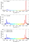Fig. B.1 The total intensity (I) spectra of the 6.7 GHz CH3OH (upper panel) and 6.035 GHz ex-OH (middle panel) maser emissions, and the left- and right-hand circular polarization (LHCP, RHCP) spectra (bottom panel) of the ex-OH maser emission detected toward G69.540-0.976 (ON 1). The systemic velocity of the region is $V_{\mathrm{L}\mathrm{S}\mathrm{R},\text{sys}}^{\mathrm{O}\mathrm{N}1}=+11.6{\mathrm{k}\mathrm{m}\mathrm{s}}^{-1}$ (Bronfman et al. 1996).

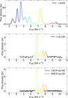Fig. B.2 Similar to Fig. B.1 but for G81.871+0.781 (W75N). The systemic velocity of the region is $V_{\mathrm{L}\mathrm{S}\mathrm{R},\mathrm{s}\mathrm{y}\mathrm{s}}^{\mathrm{W}75\mathrm{N}}=+10.0{\mathrm{k}\mathrm{m}\mathrm{s}}^{-1}$ (Shepherd et al. 2003).

References

All Tables

All Figures

Fig. 1 Distribution of 6.7 GHz CH3OH (left panels, circle symbols) and 6.035 GHz ex-OH (right panel, square symbols) maser features detected around ON 1 (top panels; $V_{\mathrm{L}\mathrm{S}\mathrm{R},\mathrm{s}\mathrm{y}\mathrm{s}}^{\mathrm{O}\mathrm{N}1}=+11.6\mathrm{k}\mathrm{m}{\mathrm{s}}^{-1}$; Bronfman et al. 1996) and W75N (bottom panels; $V_{\mathrm{L}\mathrm{S}\mathrm{R},\mathrm{s}\mathrm{y}\mathrm{s}}^{\mathrm{W}75\mathrm{N}}=+10.0\mathrm{k}\mathrm{m}{\mathrm{s}}^{-1}$; Shepherd et al. 2003). The size of the symbols is scaled logarithmically according to their peak intensity (see Tables A.1–A.4), while their colors indicate the VLSR (see Tables A.1–A.4). The reference positions are RA(J2000)=20h 10m09s.04272±0s.00007 and Dec(J2000)=+31° 31′ 34′′.9736 ± 0′.0009 for ON 1; and RA(J2000)=20h 38m 36.41744 ± 0.00008 and Dec(J2000)=+42° 37′ 35′′.1153 ± 0′.0011 for W75N. The measured linear polarization vectors with their scales, the estimated $\mathrm{\Delta }{V}_{\mathrm{Z}}^{{CH}_{3}OH}$, and the measured $B_{\parallel }^{ex-OH}$ are also reported.

In the text

	Fig. 2 Total intensity (I, upper panel) and circularly polarized intensity (V, lower panel) spectra for the 6.7 GHz CH3OH maser features named G69.M04, W75N.M21, W75N.M29, and W75N.M43 (see Tables A.1, and A.3). The thick red lines are the best-fit models of I and V emissions obtained using the adapted FRTM code (see Sect. 2). The maser features were centered on zero velocity.
In the text

Fig. B.1 The total intensity (I) spectra of the 6.7 GHz CH3OH (upper panel) and 6.035 GHz ex-OH (middle panel) maser emissions, and the left- and right-hand circular polarization (LHCP, RHCP) spectra (bottom panel) of the ex-OH maser emission detected toward G69.540-0.976 (ON 1). The systemic velocity of the region is $V_{\mathrm{L}\mathrm{S}\mathrm{R},\text{sys}}^{\mathrm{O}\mathrm{N}1}=+11.6{\mathrm{k}\mathrm{m}\mathrm{s}}^{-1}$ (Bronfman et al. 1996).

In the text

	Fig. B.2 Similar to Fig. B.1 but for G81.871+0.781 (W75N). The systemic velocity of the region is $V_{\mathrm{L}\mathrm{S}\mathrm{R},\mathrm{s}\mathrm{y}\mathrm{s}}^{\mathrm{W}75\mathrm{N}}=+10.0{\mathrm{k}\mathrm{m}\mathrm{s}}^{-1}$ (Shepherd et al. 2003).
In the text

References

- Argon, A. L., Reid, M. J., & Menten, K. M., 2000, ApJS, 129, 159 [Google Scholar]
- Bartkiewicz, A., Szymczak, M., Cohen, R. J., & Richards, A. M. S., 2005, MNRAS, 361, 623 [NASA ADS] [CrossRef] [Google Scholar]
- Bartkiewicz, A., Szymczak, M., & van Langevelde, H. J., 2016, A&A, 587, A104 [NASA ADS] [CrossRef] [EDP Sciences] [Google Scholar]
- Baudry, A., Desmurs, J. F., Wilson, T. L., & Cohen, R. J., 1997, A&A, 325, 255 [NASA ADS] [Google Scholar]
- Beuther, H., Soler, J. D., Vlemmings, W., et al. 2018, A&A, 614, A64 [NASA ADS] [CrossRef] [EDP Sciences] [Google Scholar]
- Bronfman, L., Nyman, L. A., & May, J., 1996, A&AS, 115, 81 [Google Scholar]
- Carrasco-González, C., Rodríguez, L. F., Torrelles, J. M., Anglada, G., & González-Martín, O., 2010, AJ, 139, 2433 [CrossRef] [Google Scholar]
- Carrasco-González, C., Torrelles, J. M., Cantó, J., et al. 2015, Science, 348, 114 [CrossRef] [Google Scholar]
- Cragg, D. M., Sobolev, A. M., & Godfrey, P. D., 2002, MNRAS, 331, 521 [CrossRef] [Google Scholar]
- Cragg, D. M., Sobolev, A. M., & Godfrey, P. D., 2005, MNRAS, 360, 533 [Google Scholar]
- Crutcher, R. M., & Kemball, A. J., 2019, Front. Astron. Space Sci., 6, 66 [CrossRef] [Google Scholar]
- Dall'Olio, D., Vlemmings, W. H. T., Lankhaar, B., & Surcis, G., 2020, A&A, 644, A122 [NASA ADS] [CrossRef] [EDP Sciences] [Google Scholar]
- Davies, R. D., 1974, IAU Symp., 60, 275 [Google Scholar]
- Etoka, S., Gray, M. D., & Fuller, G. A., 2012, MNRAS, 423, 647 [NASA ADS] [CrossRef] [Google Scholar]
- Fish, V. L., & Reid, M. J., 2006, ApJS, 164, 99 [NASA ADS] [CrossRef] [Google Scholar]
- Fish, V. L., & Reid, M. J., 2007, ApJ, 670, 1159 [NASA ADS] [CrossRef] [Google Scholar]
- Fish, V. L., Reid, M. J., Argon, A. L., & Zheng, X.-W., 2005, ApJS, 160, 220 [NASA ADS] [CrossRef] [Google Scholar]
- Fish, V. L., & Sjouwerman, L. O., 2010, ApJ, 716, 106 [NASA ADS] [CrossRef] [Google Scholar]
- Fish, V. L., Gray, M., Goss, W. M., & Richards, A. M. S., 2011, MNRAS, 417, 555 [NASA ADS] [CrossRef] [Google Scholar]
- Goldreich, P., Keeley, D. A., & Kwan, J. Y., 1973, ApJ, 179, 111 [NASA ADS] [CrossRef] [Google Scholar]
- Gray, M. D., Hutawarakorn, B., & Cohen, R. J., 2003, MNRAS, 343, 1067 [Google Scholar]
- Green, J. A., Richards, A. M. S., Vlemmings, W. H. T., Diamond, P., & Cohen, R. J., 2007, MNRAS, 382, 770 [NASA ADS] [CrossRef] [Google Scholar]
- Green, J. A., Caswell, J. L., & McClure-Griffiths, N. M., 2015, MNRAS, 451, 74 [NASA ADS] [CrossRef] [Google Scholar]
- Hu, B., Menten, K. M., Wu, Y., et al. 2016, ApJ, 833, 18 [Google Scholar]
- Hunter, T. R., Taylor, G. B., Felli, M., & Tofani, G., 1994, A&A, 284, 215 [Google Scholar]
- Hutawarakorn, B., Cohen, R. J., & Brebner, G. C., 2002, MNRAS, 330, 349 [CrossRef] [Google Scholar]
- Keimpema, A., Kettenis, M. M., Pogrebenko, S. V., et al. 2015, Exp. Astron., 39, 259 [NASA ADS] [CrossRef] [Google Scholar]
- Kobak, A., Bartkiewicz, A., Rygl, K. L. J., et al. 2025, A&A, 695, A149 [NASA ADS] [CrossRef] [EDP Sciences] [Google Scholar]
- Krumholz, M. R., & Federrath, C., 2019, Front. Astron. Space Sci., 6, 7 [NASA ADS] [CrossRef] [Google Scholar]
- Kumar, M. S. N., Tafalla, M., & Bachiller, R., 2004, A&A, 426, 195 [NASA ADS] [CrossRef] [EDP Sciences] [Google Scholar]
- Lankhaar, B., Groenenboom, G. C., & van der Avoird, A., 2016, J. Chem. Phys., 145, 244301 [Google Scholar]
- Lankhaar, B., Vlemmings, W., Surcis, G., et al. 2018, Nat. Astron., 2, 145 [Google Scholar]
- MacLeod, G. C., ScaliseJr., E., Saedt, S., Galt, J. A., & Gaylard, M. J. 1998, AJ, 116, 1897 [Google Scholar]
- Minier, V., Conway, J. E., & Booth, R. S., 2001, A&A, 369, 278 [NASA ADS] [CrossRef] [EDP Sciences] [Google Scholar]
- Modjaz, M., Moran, J. M., Kondratko, P. T., & Greenhill, L. J., 2005, ApJ, 626, 104 [NASA ADS] [CrossRef] [Google Scholar]
- Moscadelli, L., Sanna, A., & Goddi, C., 2011, A&A, 536, A38 [NASA ADS] [CrossRef] [EDP Sciences] [Google Scholar]
- Nagayama, T., Nakagawa, A., Imai, H., Omodaka, T., & Sofue, Y., 2008, PASJ, 60, 183 [NASA ADS] [CrossRef] [Google Scholar]
- Nammahachak, S., Asanok, K., Hutawarakorn Kramer, B., et al. 2006, MNRAS, 371, 619 [NASA ADS] [CrossRef] [Google Scholar]
- Nedoluha, G. E., & Watson, W. D., 1992, ApJ, 384, 185 [NASA ADS] [CrossRef] [Google Scholar]
- Price, D. J., & Bate, M. R., 2007, MNRAS, 377, 77 [NASA ADS] [CrossRef] [Google Scholar]
- Rodríguez-Kamenetzky, A., Carrasco-González, C., Torrelles, J. M., et al. 2020, MNRAS, 496, 3128 [Google Scholar]
- Rygl, K. L. J., Brunthaler, A., Reid, M. J., et al. 2010, A&A, 511, A2 [NASA ADS] [CrossRef] [EDP Sciences] [Google Scholar]
- Rygl, K. L. J., Brunthaler, A., Sanna, A., et al. 2012, A&A, 539, A79 [NASA ADS] [CrossRef] [EDP Sciences] [Google Scholar]
- Sault, R., 2012, EVLA Memo, 159 [Google Scholar]
- Shepherd, D. S., Testi, L., & Stark, D. P., 2003, ApJ, 584, 882 [NASA ADS] [CrossRef] [Google Scholar]
- Sugiyama, K., Fujisawa, K., Doi, A., et al. 2011, PASJ, 63, 53 [NASA ADS] [Google Scholar]
- Surcis, G., Vlemmings, W. H. T., Dodson, R., & van Langevelde, H. J., 2009, A&A, 506, 757 [NASA ADS] [CrossRef] [EDP Sciences] [Google Scholar]
- Surcis, G., Vlemmings, W. H. T., Curiel, S., et al. 2011a, A&A, 527, A48 [NASA ADS] [CrossRef] [EDP Sciences] [Google Scholar]
- Surcis, G., Vlemmings, W. H. T., Torres, R. M., van Langevelde, H. J., & Hutawarakorn Kramer, B. 2011b, A&A, 533, A47 [NASA ADS] [CrossRef] [EDP Sciences] [Google Scholar]
- Surcis, G., Vlemmings, W. H. T., van Langevelde, H. J., & Hutawarakorn Kramer, B., 2012, A&A, 541, A47 [NASA ADS] [CrossRef] [EDP Sciences] [Google Scholar]
- Surcis, G., Vlemmings, W. H. T., van Langevelde, H. J., Hutawarakorn Kramer, B., & Bartkiewicz, A., 2019, A&A, 623, A130 [NASA ADS] [CrossRef] [EDP Sciences] [Google Scholar]
- Surcis, G., Vlemmings, W. H. T., van Langevelde, H. J., Hutawarakorn Kramer, B., & Bartkiewicz, A., 2022, A&A, 658, A78 [NASA ADS] [CrossRef] [EDP Sciences] [Google Scholar]
- Surcis, G., Vlemmings, W. H. T., Goddi, C., et al. 2023, A&A, 673, A10 [NASA ADS] [CrossRef] [EDP Sciences] [Google Scholar]
- Szymczak, M., Olech, M., Sarniak, R., Wolak, P., & Bartkiewicz, A., 2018, MNRAS, 474, 219 [Google Scholar]
- Szymczak, M., Wolak, P., Bartkiewicz, A., Aramowicz, M., & Durjasz, M., 2020, A&A, 642, A145 [NASA ADS] [CrossRef] [EDP Sciences] [Google Scholar]
- Torrelles, J. M., Gómez, J. F., Rodríguez, L. F., et al. 1997, ApJ, 489, 744 [Google Scholar]
- Vlemmings, W. H. T., 2008, A&A, 484, 773 [NASA ADS] [CrossRef] [EDP Sciences] [Google Scholar]
- Vlemmings, W. H. T., Surcis, G., Torstensson, K. J. E., & van Langevelde, H. J., 2010, MNRAS, 404, 134 [NASA ADS] [Google Scholar]
- Vlemmings, W. H. T., Torres, R. M., & Dodson, R., 2011, A&A, 529, A95 [NASA ADS] [CrossRef] [EDP Sciences] [Google Scholar]
- Zheng, X. W., Ho, P. T. P., Reid, M. J., & Schneps, M. H., 1985, ApJ, 293, 522 [Google Scholar]
The name follows the Galactic coordinates of the target.
All Tables
Comparison of the magnetic field along the line of sight as measured from the Zeeman splitting of the 6.7 GHz CH3OH, considering three different hyperfine transitions, and 6.035 GHz ex-OH maser features in ON 1 and W75N.
Parameters of the 6.7 GHz CH3OH maser features detected in G 69.540–0.976 (ON 1).
Parameters of the 6.035 GHz ex-OH maser features detected in G69.540-0.976 (ON 1).
Parameters of the 6.7 GHz CH3OH maser features detected in G 81.871+0.781 (W75N).
Parameters of the 6.035 GHz ex-OH maser features detected in G81.871+0.781 (W75N).