| Issue |
A&A
Volume 701, September 2025
|
|
|---|---|---|
| Article Number | A76 | |
| Number of page(s) | 9 | |
| Section | Interstellar and circumstellar matter | |
| DOI | https://doi.org/10.1051/0004-6361/202555773 | |
| Published online | 04 September 2025 | |
Prospects for studying million-degree gas in the Milky Way halo using the forbidden optical [Fe X] and [Fe XIV] intersystem lines
1
Institut für Physik und Astronomie, Universität Potsdam,
Karl-Liebknecht-Str. 24/25,
14476
Golm,
Germany
2
Department of Physics and Astronomy, University of Notre Dame,
Notre Dame,
IN
46556,
USA
3
European Southern Observatory (ESO),
Karl-Schwarzschildstrasse 2,
85748
Garching,
Germany
4
Aix Marseille Université, CNRS, LAM (Laboratoire d’Astrophysique de Marseille) UMR 7326,
13388
Marseille,
France
5
Leibniz-Institut für Astrophysik Potsdam (AIP),
An der Sternwarte 16,
14482
Potsdam,
Germany
★ Corresponding author: This email address is being protected from spambots. You need JavaScript enabled to view it.
Received:
2
June
2025
Accepted:
16
July
2025
Abstract
Context. The Milky Way is surrounded by large amounts of hot gas at temperatures of T > 106 K, which represents a major baryon reservoir.
Aims. We explore the prospects of studying the hot coronal gas in Milky Way halo by analyzing the highly forbidden optical coronal lines of [Fe X] and [Fe XIV] in absorption against bright (unrelated) extragalactic background sources.
Methods. We used a semi-analytic model of the Milky Way’s coronal gas distribution together wih HESTIA simulations of the Local Group and observational constraints to predict the expected Fe X and Fe XIV column densities, as well as the line shapes and strengths for the [Fe X] λ6374.5 and [Fe XIV] λ5302.9 transitions. We provide predictions for the signal-to-noise ratio (S/N) required to detect these lines. Using archival optical data from an original sample of 739 high-resolution AGN spectra from VLT/UVES and KECK/HIRES, we generated a stacked composite spectrum to measure an upper limit for the column densities of Fe X and Fe XIV in the Milky Way’s coronal gas.
Results. We predicted column densities of log N(Fe X) = 15.40 and log N(Fe XIV) = 15.23 in the Milky Way’s hot halo, corresponding to equivalent widths of WFeX, 6347 = 190 μÅ and WFeXIV, 5302 = 220 μÅ. We estimated that a minimum S/N of ∼50 000(∼25 000) is required to detect [Fe X] λ6374.5 ([Fe XIV] λ5302.9) absorption at a 3σ level. There was no [Fe X] and [Fe XIV] detected in our composite spectrum, which achieves a maximum S/N = 1240 near 5300 Å. We derived 3σ upper column-density limits of log N(Fe X) ≤ 16.27 and log N(Fe XIV) ≤ 15.85, in line with the above-mentioned predictions.
Conclusions. While [Fe X] and [Fe XIV] absorption is too weak to be detected with current optical data, we outline how upcoming extragalactic spectral surveys with millions of medium- to high-resolution optical spectra will provide the necessary sensitivity and spectral resolution to measure velocity-resolved [Fe X] and [Fe XIV] absorption in the Milky Way’s coronal gas (and beyond). This opens up a new prospective window on studies of the dominant baryonic mass component of the Milky Way taking the form of hot coronal gas via optical spectroscopy.
Key words: atomic processes / techniques: spectroscopic / Galaxy: halo
© The Authors 2025
 Open Access article, published by EDP Sciences, under the terms of the Creative Commons Attribution License (https://creativecommons.org/licenses/by/4.0), which permits unrestricted use, distribution, and reproduction in any medium, provided the original work is properly cited.
This article is published in open access under the Subscribe to Open model. This email address is being protected from spambots. You need JavaScript enabled to view it. to support open access publication.
1 Introduction
The dominant baryonic mass reservoir in galaxies is the diffuse gas contained within their halos, known as the circumgalactic medium (CGM). It plays a crucial role in the ongoing formation and evolution of galaxies and now stands as a major research field in modern astrophysics (Tumlinson et al. 2017).
As a consequence of the highly complex physics involved (e.g., full magnetohydrodynamics, cosmic rays, nonequilibrium cooling and heating, etc.) and the dynamics of the processes that contribute to its mass and energy budget, the CGM is an extremely heterogeneous gaseous medium undergoing multiple phases. In the simplified picture, the CGM is composed of cool and warm (T = 102–105 K) streams of gas that are embedded in a hotter gaseous medium (T = 106–107 K). As observations of the Milky Way’s CGM have indicated, the dimensions of circumgalactic gas features range from AU scales (in high-density clumps; Richter et al. 2003; Meyer & Lauroesch 1999) to several hundred kiloparsecs (in large, coherent gas streams such as the Magellanic Stream; Putman 2003; Richter 2017). It is only in the context of the Milky Way that the CGM can be observationally resolved at all these scales, making our Galaxy an important testing ground for our general understanding of the CGM. On the other hand, this enormous dynamic range in physical conditions and spatial scales makes it challenging for magnetohydrodynamic simulations to offer a realistic picture of CGM in all its facets (see Crain & van de Voort 2023, and references therein).
Global CGM properties of Milky Way type galaxies can be modeled in the context of ΛCDM galaxy formation models (White & Frenk 1991; Naab & Ostriker 2017), where predictions suggest that diffuse gas in cosmological filaments is accreted onto dark matter halos and shock-heated to approximately the halo virial temperature (a few million degrees for Milky-Way type galaxies). This hot gas is sometimes referred to as the “galactic corona,” analogously to the Sun’s hot coronal gas (Spitzer 1956). Cooling processes from the coronal gas, stripping of satellite galaxies, and accretion of metal-poor gas from the intergalactic medium (IGM) lead to the formation cold gas streams that move toward the disk where the gas is cooled and transformed into stars or is fueling the coronal gas of more massive galaxies (Afruni et al. 2023). In addition to the accretion of material from the corona and from outside, gas (along with energy) is also ejected into the CGM from inside from the disk as a result of feedback processes (Marasco et al. 2022) after which it is re-accreted onto the disk. Therefore, the CGM is believed to represent a substantial baryon reservoir that reflects the evolutionary state of its host galaxy (Péroux & Howk 2020).
With its low gas densities (log nH = −2 to −5, typically) and high temperatures (T > 106 K), the hot coronal gas phase is particularly difficult to observe (Comparat et al. 2022). For the Milky Way, the X-ray transitions of O VII, O VIII, and other high ions provide important diagnostic lines to study the Galaxy’s hot coronal gas component. These lines can be observed either in absorption against X-ray bright active galactic nuclei (AGNs) or in emission (Fang et al. 2006; Miller & Bregman 2013, 2015; Hodges-Kluck et al. 2016; Li & Bregman 2017; Das et al. 2021). Recent X-ray studies indicate that the Milky Way’s hot coronal gas contains a total mass of as much as ∼1011 M⊙ within 250 kpc (e.g., Miller & Bregman 2013, 2015). A major drawback of CGM X-ray observations is, however, the very low spectral resolution of the data, which precludes a precise localization of the hot gas resevoirs within the Milky Way, its circumgalactic environment, and in the Local Group (Bhattacharyya et al. 2023), offering only limited information on its overall dynamics.
Unlike in the X-ray band, there are no strong resonance lines from highly ionized metals available in the ultraviolet (UV) and optical regime that would independently trace million-degree gas in the CGM and IGM at z = 0 in a direct manner. Indirect methods to trace hot gas in the Local Universe in the CGM and IGM via intermediate-and high-resolution UV absorption spectroscopy include the measurements of transition-temperature gas (T ∼ 105.5 K) using the O VI doublet (Sembach et al. 2003; Savage et al. 2003; Tripp et al. 2008) and the analysis of thermally broadened H I Ly α absorption lines (BLAs) and coronal BLAs (CBLAs) that trace the tiny neutral gas fraction in the hot medium (Richter et al. 2006a, b; Lehner et al. 2007; Tepper-García et al. 2012; Richter 2020). For the study of the CGM of the Milky Way and other Local Group member galaxies, the analysis of CBLAs is not an option, however, as the damped interstellar H I Ly α absorption superposes any CBLA signature within |vLSR| ≈ 700 km s−1. High-ion transitions in the extreme UV, such as Ne VIII λλ770.4, 780.3, cannot be used to trace hot gas in the z = 0 Universe, but are accessible only at higher redshifts (Tepper-García et al. 2014).
A potential alternative to strong resonance lines are (exceedingly weak) forbidden transitions of high-ions, the most prominent of them (from early studies of the Sun) being located in the optical regime. Already in the 1980s, York & Cowie (1983) discussed the possibility to use the intersystem lines of [Fe X] near 6375 Å and [Fe XIV] near 5303 Å as the most promising candidate lines from the set of forbidden transitions in the optical regime to sample shock-heated, hot gas in the CGM and IGM in optical spectra from ground-based telescopes. However, because of the very small oscillator strengths of these forbidden transitions, an extremely high S/N of a few thousand would be required to detect these lines in the spectra of background AGNs, which is (so far) not feasible for individual targets. In collisional ionization equilibrium, these lines trace gas at temperatures T = 106.0–106.3 K (see Fig. 1), which is close to the halo virial temperature of Milky-Way type galaxies (see above). In the 1980s, several groups searched for [Fe X] at λ6374.5 and [Fe XIV] λ5302.9 absorption in the Milky Way ISM and in hot gas toward the LMC (Hobbs 1984; Hobbs & Albert 1984; Hobbs 1985; Pettini & D’Odorico 1986; Wang et al. 1989; Pettini et al. 1989; Malaney & Clampin 1988), but none of them found a convincing signal (despite the inital claims of a detection; see discussion in Sect. 2.2). In complementing these optical studies, Anderson & Sunyaev (2016, 2018) have investigated emission signatures of hot gas around the nucleus of M87 using the highly forbidden transition of [Fe XXI] in the far UV at 1354.1 Å.
In Richter et al. (2014), we discussed the possibility of using the [Fe X] λ6374.5 and [Fe XIV] λ5302.9 lines in stacks of archival optical spectra of extragalactic sight lines from VLT/UVES to put constraints on the hot gas mass in the Milky Way coronal gas. There are several compelling reasons to seriously consider these transitions for a systematic study of the Milky Way’s hot coronal gas: (i) detecting [Fe X] and/or [Fe XIV] would offer independent constraints on the mass of hot gas in and around the Milky Way, complementing other measurement methods; (ii) acquiring the necessary data incurs no additional cost, as they will be readily available from numerous ongoing and upcoming extragalactic spectral surveys; (iii) even deep optical surveys can provide relatively high spectral resolution, enabling detailed insights into the velocity profile of the absorbing gas, as well as its position relative to the Milky Way’s disk, central region, and large-scale environment, which is kinematic information that other methods cannot provide; iv) when combined with observations from other probes, such as fast radio bursts (FRBs), these data might help to constrain the iron abundance in the Milky Way’s hot corona and shed light on the enrichment history of this gas. Zastrocky et al. (2018) stacked KECK/HIRES spectra from the KODIAQ sample to provide a first upper column-density limit for Fe XIV in the Milky Way halo; however, their limit is more than two orders of magnitude above the expected level.
Motivated by the many upcoming spectroscopic galaxy surveys from other instruments, which will provide millions of medium- to high-resolution spectra, we chose to revisit this idea in this work and provide, for the first time, testable predictions for the expected stengths of the [Fe X] λ6374.5 and [Fe XIV] λ5302.9 absorption lines from the Galaxy’s hot coronal gas based on models, simulations, and observations of the distribution of the CGM in the Milky Way halo.
This paper is organized as follows. In Sect. 2, we review the physical properties of the [Fe X] λ6374.5 and [Fe XIV] λ5302.9 lines and discuss the results from previous attempts of detecting them. In Sect. 3, we discuss the hot gas distribution in the Milky Way halo and constrain the expected hot gas column density from an analytic model, from the HESTIA simulations of the Local Group and from dispersion measurements. In Sect. 4, we present our predictions for the expected absorption strength of these two lines and provide upper limits for the column densities of log N(Fe X) and log N(Fe XIV) from a combined stack of VLT/UVES and KECK/HIRES. We discuss the prospects of detecting [Fe X] λ6374.5 and [Fe XIV] λ5302.9 absorption in stacked spectra from upcoming spectroscopic surveys in Sect. 5. Our summary and conclusions are given in Sect. 6.
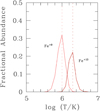 |
Fig. 1 Fractional abundances of Fe+9 and Fe+13 in a collisional ionization equilibrium (from Bryans et al. 2009, see also Sect. 2.1). |
2 Tracing million degree gas with [Fe X] and [Fe XIV] absorption
2.1 Constraints from atomic physics
The optical intersystem transitions of [Fe X] at λ0 = 6374.51 Å and [Fe XIV] at λ0 = 5302.86 Å (Shirai et al. 2000)1 are magnetic dipole transitions (M1) that are well known from observations of the solar corona, where these transitions lead to prominent emission features: the “coronal” lines, known since 1939 (Grotrian 1939). In contrast to the high density (nH ∼ 105 cm−3) coronal plasma of the Sun, the forbidden optical intersystem transitions of [FeX] and [FeXIV] can be detected in hot, low-density intergalactic and circumgalactic gas (typically nH < 10−4 cm−3) only in absorption against extragalactic background sources (such as quasars and quasi-stellar objects, QSOs, and other type of AGNs).
The expected line strengths of [Fe X] λ6374.5 and [Fe XIV] λ5302.9 absorption in a given hot-gas distribution depend on i) the total gas column density; ii) the local iron abundance in the gas; iii) the fractional abundances of the Fe X and Fe XIV ions (e.g., dictated by the temperature in collisional ionization equilibrium); and iv) the transition probabilities (oscillator strengths) of the λ6374.5 and λ5302.9 transitions. In the following, we discuss all of these parameters and their relation to each other in preparation for our predictions of the [Fe X] and [Fe XIV] line strengths in the hot coronal gas of the Milky Way (Sect. 4.1).
The total column density, Ntot ≈ N(H), of million-degree coronal gas around the Milky Way (and other galaxies) has only partly been determined by X-ray observations (see introduction section). However, it can be estimated from analytic halo models and cosmological (magneto)hydrodynamical simulations as well as from measurements of the dispersion measure against extragalactic FRBs (discussed in detail in Sect. 3).
The local iron abundance in the gas, (Fe/H)Cor, can be expressed in terms of the solar iron abudance (Fe/H)⊙ = 3.16 × 10⁻⁵; Asplund et al. 2009), so that (Fe/H)Cor ≡ XFe(Fe/H)⊙ with XFe as free parameter to be defined. The fractional abundances of FeX and Fe XIV in the gas, fFeX and fFeXIV, depend on the ionization state of the medium (and is thus driven by the ionization mechanisms). It requires very high energies of 234 eV to ionize Fe+8 to Fe+9 and 361 eV from Fe+12 to Fe+13 (e.g., Sutherland & Dopita 1993).
In the absence of an intense flux of extremely hard photons (as expected in most astrophysical environments, particularly in the CGM and IGM), collisional ionization at million-degree temperatures is the only mechanism that is expected to produce a significant population of Fe+9 and Fe+13 ions in diffuse intergalactic and circumgalactic gas. Assuming collisional ionization equilibrium (CIE) and adopting CIE models for Fe X and Fe XIV from Bryans et al. (2009), the maximum fractional abundance of Fe X at its CIE peak temperature (Tp,FeX = 1.0 × 10⁶ K) is pFeX = 0.32. Meanwhile, for Fe XIV, it is pFeXIV = 0.22 at. Tp,FeXIV) = 2.0 × 10⁶ K (see Fig. 1). We note that these fractional abundances do not change significantly (Δ p ≤ 0.002) if we consider nonequilibrium collisional ionization models, such as those presented in Gnat & Sternberg (2007). With Einstein coefficients of Aki = 69.4 s−1 and Aki = 60.2 s−1 (Fuhr et al. 1988), the transitions of [Fe X] λ6374.5 and [Fe XIV] λ5302.9 have extremely small oscillator strengths, fλ6374 = 2.1 × 10⁻⁷ and fλ5302 = 5.1 × 10⁻⁷.
For a weak, unsaturated absorption line of an ion, Y, there is a simple, linear relation between the observed equivalent width, Wλ, and the ion column density, N(Y), in the gas, expressed as
 (1)
(1)
Here, λ0 denotes the laboratory wavelength of the transition and f its oscillator strength.
At their respective CIE peak temperatures, the column densities of Fe X and Fe XIV can then be expressed as N(Fe X) = pFeX XFe(Fe/H)⊙ N(H) = 1.01 × 10⁻⁵ XFe N(H) and N(Fe XIV)= pFeXIV XFe(Fe/H)⊙ N(H) = 6.95 × 10⁻⁶ XFe N(H), so that
 (2)
(2)
and
 (3)
(3)
We see that for a 1 mÅ absorption line to arise in the [Fe X] λ6374.5 ([Fe XIV] λ5302.9) line it requires a total ionized gas column density as large as 1.3 × 1021 cm−2(1.1 × 1021 cm−2) at a solar Fe iron abundance. Because of the high gas temperature, the resulting absorption lines will be substantially broadened. The expected thermal Doppler parameter would then be
 (4)
(4)
In this equation, k is the Boltzmann constant, mion is the ion mass, and A is the relative atomic mass of the absorbing ion. In the case of Fe, AFe = 55.815 (see the NIST Atomic Spectra Lines Database; Kramida et al. 2023), so that for a gas temperature of T=106 K(2 × 10⁶ K), we have bth = 17 km s−1(24 km s−1). We note that because of the relatively high mass of iron, this bth value is substantially smaller than the bth values expected for thermally broadened H I Ly α absorbers in the CGM (AH=1; Richter 2020). The expected small breadth of the Fe lines favours their detectability in a typical AGN continuum spectrum that is altered with noise features (see Fig. 2).
Because bth values are predicted to be relatively small for the Fe lines, nonthermal broadening mechanisms (e.g., from the differential co-rotation of the coronal gas with the disk and bulk motions of the hot gas) are expected to be important. Such nonthermal motions are commonly parameterized with bnth, so that the expected observed Doppler parameter b is composed of both of these components,  . The actual contribution of bnth to b is challenging to estimate without knowing the systematic large-scale motions and the internal velocity dispersion of the hot gas in the corona.
There is observational evidence that the hot corona is partly co-rotating with the underlying disk (Hodges-Kluck et al. 2016). However, the implication of such a systematic motion along a line of sight from the Sun to Milky Way’s virial radius for the shape of the Fe absorption lines is unclear, since it remains to be determined how the rotation speed scales with the vertical height of the hot gas layers. The role of nonthermal gas motions for b are further discussed in Sect. 3.2, where we analyze the velocity dispersion of the coronal gas in the HESTIA simulations.
For a given equivalent width, the central absorption depth, , of an absorption line depends on its width and thus on b. Following Richter (2020), we can express the following, assuming a Gaussian shape:
![Mathematical equation: $\mathcal{D}=0.139\left[\frac{W_{\lambda}}{\mathrm{m{\mathop{\mathrm{A}}^{\circ}}}}\right]\left[\frac{b}{\mathrm{~km} \mathrm{~s}^{-1}}\right]^{-1}.$](/articles/aa/full_html/2025/09/aa55773-25/aa55773-25-eq7.png) (5)
(5)
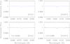 |
Fig. 2 Synthetic spectra of the [Fe X] at λ6374.5 and [Fe XIV] λ5302.9 lines from our halo model described in Sect. 4.1. The upper two panels show the noise-free absorption profiles, the lower two panels show the profiles with the minimum S/N required for a 3σ detection, as given in the lower left corners. The spectra are generated using a spectral resolution of R = 45 000 and a sampling of 1.5 pixels per resolution element. |
2.2 Previous [Fe X] and [Fe XIV] observations
In light of the values obtained in the previous subsection, we discuss the results from previous studies of [Fe X] and [Fe XIV] absorption in nearby hot gas and toward the Magellanic Clouds. Even 40 years ago, (Hobbs 1984; Hobbs & Albert 1984; Hobbs 1985; Pettini & D’Odorico 1986) searched for [Fe X] and [Fe XIV] absorption in the local Milky Way ISM using the high-S/N spectra of nearby stars. These studies did not find any convincing signal down to a level of ∼ 1 mÅ. However, million-degree gas within the Milky-Way gas disk is expected to reside only in localized environments on sub-kiloparsec scales (e.g., the local hot bubble or other supernova bubbles and chimneys) that do not provide sufficient column density for [Fe X] and [Fe XIV] absorption to be detected at a ∼ 1 mÅ level (e.g., Liu et al. 2017). This is because for a hot-gas density as high as nH=10−2 cm−3, it requires an absorption path length of 3.2 kpc to achieve a hydrogen column density of N(H) = 1020 cm−2. Therefore, the reported nondetections in the above-listed studies are consistent with Equations (2) and (3).
From the analysis of the optical spectrum of the extremely bright supernova SN 1987A in the LMC, several groups (Wang et al. 1989; Pettini et al. 1989; Malaney & Clampin 1988) reported the detection of a weak (Wλ ∼ 3 mÅ) absorption feature near 6380 Å that was identified as Doppler-shifted [Fe X] λ6374.5 absorption arising from hot gas in the direction of the LMC (Pettini et al. 1989). If true, this would imply a large column of ionized gas in this direction, log N(H II) ≈ 21.5 (Eq. (2)), indicating the existence of a huge reservoir of baryonic matter hidden in hot gas. The interpretation of the observed absorption feature near 6380 Å as [Fe X] absorption was, however, disputed by Wampler et al. (1991), who identified the observed feature as a Doppler-shifted diffuse interstellar band (DIB). There are several weak DIBs and telluric lines present in the optical regions in which the [Fe X] λ6374.5 and [Fe XIV] λ5302.9 lines are located (see, e.g., Jenniskens & Desert 1994). The latter interpretation appears more likely, because the existence of a uniform layer of million-degree gas around the LMC at a column density of log N(H II) ≈ 21.5 would imply an enormously high baryon-to-dark-matter ratio that is not in line with current galaxy formation models. Such a large ionized gas column density is also not supported by UV and X-ray observations of hot gas in the general direction of the LMC (Krishnarao et al. 2022; Locatelli et al. 2024).
More recently, Richter et al. (2014) discussed high-S/N VLT/UVES observations of high-redshift QSOs as possible probes for [Fe X] and [Fe XIV] absorption in the Milky Way’s coronal gas (e.g., their Fig. 4). They also proposed stacking techniques for UVES high-resolution and SDSS low-resolution archival spectra to achieve the required S/N levels. From the stacking of 95 pre-selected Keck HIRES spectra, Zastrocky et al. (2018) derived 3σ upper limits for [Fe XIV] absorption in the Milky Way halo of W5302 ≤ 7 mÅ and N(Fe XIV) = 5.5 × 1016 cm−2 achieving a S/N of ∼ 300.
3 Expected properties of the Milky Way’s hot coronal gas
To determine realistic expectation values for W6347 and W5302 from [Fe X] and [Fe XIV] absorption in the Milky Way’s hot coronal gas, we need to estimate N(H) for the coronal gas at the CIE peak temperatures of Fe+9 to Fe+13 (Fig. 1) in the range log T = 6.0–6.3 (see Eqs. (2) and (3)) for extragalactic sight lines from the vantage point of the Sun. For this, we used (i) the semi-analytic model of the hot gas distribution around low-redshift galaxies from Richter (2020); (ii) results from the constrained magneto-hydrodynamical simulation of the Milky Way and Local Group as part of the HESTIA project (Libeskind et al. 2020; Damle et al. 2022; Rünger et al. 2025); and (iii) constraints from measurements of the dispersion measure of gas in and around the Milky Way using FRBs (Cook et al. 2023).
3.1 Constraints from a semi-analytic model
In Richter (2020), we used a semi-analytic approach to model the spatial density and temperature distribution of hot coronal gas of galaxies with virial halo masses in the range log (M/M⊙) = 10.6–12.6 to predict the strength, spectral shape, and cross section of the CBLAs as a function of galaxy-halo mass and line-of-sight impact parameter from an external vantage point. In this model, it is assumed that the hot coronal gas is confined in a dark-matter halo that follows a Navarro-Frenk-White (NFW) density profile (Navarro et al. 1995; Klypin et al. 2001). After the initial collapse, the gas is assumed to be shock-heated to the halo’s virial temperature and then cools within a characteristic cooling radius to become multi-phase (see Maller & Bullock 2004, for a detailed description of the original equations).
To model the spectral signatures of such gas along the QSO sight lines, we then have applied the halopath code, as originally described in Richter (2012). The same approach and modeling codes were used here to calculate N(H) for T ≥ 106 K in a Milky-Way mass halo from any given vantage point inside the halo by integrating nH from the initial position out to the virial radius, Rvir.
For the Milky Way mode halo, we adopted a halo mass of log (M/M⊙) = 12.0 and a virial radius of Rvir = 250 kpc. For the sake of simplicity, we assumed the observer to be located in the geometrical center of the spherical model halo (for more details about the model see Richter 2020). If we only consider gas with T ≥ 106 K, the total hydrogen column density of that gas between R = 0 kpc and Rvir is typically N(H I) = 1.0 × 1020 cm−2. To put this number into context: a similar column density is observed for neutral hydrogen in the Magellanic Stream (e.g., Putman 2003; Fox et al. 2013; Richter et al. 2013), where the absorption pathlength through the stream is substantially smaller (a few kpc, at most), but the gas density is significantly higher (as is the neutral gas fraction) as well as in the lowest N(H I) directions in the Milky Way disk; for instance, in the Lockman hole (Richter et al. 2001).
3.2 Constraints from the HESTIA simulations
While the semi-analytic halo model discussed above provides important insights into the overall hot gas distribution in the CGM as a function of halo mass, it cannot deliver information on the kinematics of the absorbing gas cells, nor can it account for density and temperature fluctuations in the hot CGM that are expected to arise due to the specific cosmological environment of the host galaxy and because of feedback processes from supernovae and AGN activity. Therefore, for a more realistic estimate of N(H) in the hot CGM of a Milky-Way type galaxy, we consider magneto-hydrodynamical (MHD) high-resolution simulations of galaxies in a cosmological context.
We make use of the suite of simulations from the Highresolution Environmental Simulations of The Immediate Environment (HESTIA) project (Libeskind et al. 2020) to systematically investigate the properties of the (simulated) Milky Way CGM (Damle et al. 2022; Biaus et al. 2022; Rünger et al. 2025). HESTIA provides representative magnetohydrodyanmical simulations of Milky Way-mass galaxies in their proper cosmographic environments using the AREPO moving-mesh code (Springel 2010) and the AURIGA galaxy evolution model (Grand et al. 2017). For more details on HESTIA, we refer to Libeskind et al. (2020).
Here, we used the three HESTIA simulations to estimate N(H) in the coronal gas from a Sun-like position at 8 kpc galactocentric distance within the (simulated) MW disk and pinpoint the velocity dispersion of the hot-gas pockets in the CGM along the various sight lines to constrain the nonthermal contribution to the Doppler parameter (Sect. 2.1). For each of the three MW simulations, we constructed 100 randomly distributed sight lines from the position of the Sun that extend to Rvir and derived N(H) by integrating over the density distribution along each sight line. As for the semi-analytic model, we restrict our analysis to gas with temperatures T ≥ 106 K. The median value for N(H) from all 300 sight lines is N(H) = 5 × 1020 cm−2. Interestingly, this value is ∼ 5 times higher than N(H) estimated from the simple semi-analytic model (Sect. 3.1). The larger column density of hot, ionized gas in the HESTIA simulation comes from the important contributions of hot gas cells related to the Milky Way’s (simulated) disk-halo interface, where supernova feedback adds to the energy and hot-baryon budget of gas in the lower halo, and possibly from gas related to Milky Way satellites within Rvir (see also Damle et al. 2025).
The (radial) velocity dispersions of the hot gas cells along the 300 sight lines vary between 30 and 128 km s−1 with a median value of ⟨σv⟩ = 50 km s−1. We regard this latter value as a characteristic velocity dispersion for the nonthermal gas motions along a typical halo sight line, which then dominates the expected line width of the [Fe X] and [Fe XIV] absorption (Sect. 2.1).
3.3 Constraints from FRBs
Another, independent constraint on the mass and extent of the hot gas in the the Milky Way halo comes from FRBs (Lorimer et al. 2007) and distant pulsars, using the well-known dispersive effect of charged particles on radio waves. By precisely measuring the arrival times of radio pulses (e.g., from pulsars or FRBs), the dispersive delay can be quantified using a quantity called the dispersion measure (DM). Since free electrons by far dominate the dispersion in a given ionized gas volume, the DM is proportional to the electron column density in the gas along a line of sight of length, L,
 (6)
(6)
Because hydrogen is the main electron donor in a fully ionized interstellar or intergalactic plasma at solar or subsolar metal abundance, we have N(e−) ≈ N(H), so that the DM is a direct measure of the total (ionized) gas mass along a line of sight.
The DM measurements deliver information on the total ionized gas column toward a background FRB or pulsar. However, they do not provide any information on how the particles are distributed along the line of sight. To localize the hot gas in and around the Milky Way and estimate its mass, the combination of many FRBs and/or pulsar sight lines of different lengths is required (see, e.g., Prochaska & Zheng 2019). From a sample of 93 FRBs for Galactic latitudes |b| ≥ 30 deg from the CHIME/FRB project, Cook et al. (2023) derived a range of DM=88–141 pc cm−3. These values correspond to a range in total ionized gas column densities of N(H)= 2.7–4.4 × 1020 cm−2; thus, slightly below the value estimated from the HESTIA simulations, but clearly above the one derived from the semi-analytic model.
4 Observational limits
4.1 Expected line strengths and profiles
If we assume a total hydrogen column density in the Milky Way’s hot coronal gas of N(H) = 5 × 1020 cm−2 and an iron abundance in the corona of half of the solar value (Martynenko 2022), the expected line strengths from Equations (2) and (3) come out as W6374=190 μ Å and W5302 = 220 μ Å. The corresponding Fe x and Fe XIV column densities are log N(Fe X) = 15.40 and log N(Fe XIV) = 15.23. For a hot-gas temperature of 2 × 10⁶ K and nonthermal gas motions characterized by bnt = 50 km s−1 (from the HESTIA simulations, see above), the expected total Doppler parameter is b = 58 km s−1.
To visualize the optical appearance of such weak spectral features, we have generated synthetic spectra of the [Fe X] λ6374.5 and [Fe XIV] λ5302.9 lines in Fig. 2 using a spectral resolution of R = 45 000 and a sampling of 1.5 pixels per resolution element. The upper two panels show the blank (noise-free) absorption profiles, for the lower two panels we have added noise at a level, that a 3σ detection of these features is realized. As we can see, a S/N of ∼ 50 000 is required to significantly detect [Fe X] absorption at the expected level, for [Fe XIV] it is ∼ 25 000.
4.2 Stacking of archival high-resolution optical AGN spectra
Even with the most efficient spectrographs on 8–10 m class telescopes, it is unrealistic to achieve the required S/N of >20 000 for a medium- to high-resolution (R ≥ 15 000) optical spectrum of an individual extragalactic background source within reasonable integration times. For the UVES spectrograph, for instance, D’Odorico et al. (2016) and Kotuš et al. (2017) presented high-resolution (R ≥ 45 000) spectra of the high-redshift QSOs HE 0940-1050 and HE 0515–4414, respectively. These data have S/N ratios of ∼500–600 per resolution element and are based on many individual pointings totaling several dozen hours of integration time with the VLT. To our knowledge, there are no other VLT/UVES (or KECK/HIRES) spectra of an individual QSO that provide a S/N significantly higher than these values.
Because every extragalactic sight line passes the Milky Way halo, however, stacking clearly is the most promising approach to achieve S/N ratios larger than 1000 for a Milky Way composite spectrum. Using low-resolution (R ∼ 2200) SDSS spectral data from stars, galaxies and quasars, Lan et al. (2015) and Murga et al. (2015) have achieved a S/N of several thousand by stacking a few hundred thousand SDSS spectra to investigate interstellar DIBs and Ca II absorption in the Milky Way foreground gas. They did not, however, find any evidence for [Fe X] and [Fe XIV] absorption in their stacked data set (Menard, priv. comm.; see also Lan et al. 2015, their Fig. 2), which is in line with the predicted strength of the absorption as calculated above. We also note that the spectral resolution of SDSS (R = 2200–2850, equivalent to Δ v ≥ 136 km s−1) is not sufficient to resolve the two [Fe X] and [Fe XIV] lines at the expected widths.
Zastrocky et al. (2018) used a sample of 95 KECK/HIRES spectra from the KODIAQ survey (O’Meara et al. 2017) for a spectral stack to search for [Fe XIV] absorption in the Milky Way halo. These authors achieved a S/N of ∼ 300 and a column density limit of log N(Fe XIV) ≤ 16.78 from the mean stack of their composite spectrum, which is far below (two orders of magnitude in terms of S/N) the required sensitivity.
For this paper, we have combined the KECK/HIRES spectra from the KODIAQ data basis with VLT/UVES spectra from the SQUAD project (Murphy et al. 2019) and other archival VLT/UVES data. Our goal is to boost the detection limit for [Fe X] and [Fe XIV] absorption from a high-resolution composite spectrum that is based on high-quality data from two of the most powerful optical spectrographs installed on 8–10 m class telescopes currently available. Both spectral datasets have similar spectral resolution R ∼ 30 000–60 000, but the average S/N in the VLT/UVES spectral data is 2–3 times higher than for the KECK/HIRES data including some spectra with exceptionally high S/N (see above) from the monitoring of AGN variability. We note that we have previously used VLT/UVES spectra from the SQUAD project to systematically investigate Ca II H & K absorption in the Milky Way halo (Richter et al. 2005; Ben Bekhti et al. 2008, 2012), in the low-redshift IGM (Richter et al. 2011), and in selected Damped Lyman- α absorbers (Guber & Richter 2016; Guber et al. 2018). Therefore, we are highly familiar with the data quality issues of the SQUAD database.
For the stacking, we developed a custom routine that identifies (in a fully automated fashion) blending features from intervening absorbers in the spectral regions near 5300 and 6375 Å. It then performs data quality checks and determines the local S/N. Using pre-defined selection criteria and bin sizes, the code then bins the data and stacks the selected spectra, where each spectrum is weighted by the inverse variance from the noise statistics in the regions around the two Fe lines. In our case, the initial sample contains 439 UVES and 300 HIRES spectra (i.e., 739 in total). Before stacking, we preselected spectra that i) have no contaminating blending line within ± 500 km s−1 of the laboratory wavelength of the [Fe X] and [Fe XIV] lines and ii) (each) having S/N ≥ 20 per resolution element. This selection leaves us with 183 spectra for [Fe X] and 156 spectra for [Fe XIV] to carry out the stacking procedure. Before stacking, the individual spectra were rebinned to achieve a homogeneous sampling, where the bin size was set as 20 km s−1, which is sufficient to resolve an absorption line that has an expected Doppler parameter of b ≥ 50 km s−1. Finally, the stacked spectrum was normalized in the regions of interest using a linear continuum fit. The resulting composite velocity profiles for the [Fe X] and [Fe XIV] lines after stacking are shown in Fig. 3. For [Fe XIV], seen in the bottom panel, the stacked composite at 5302 Å is featureless and achieves a very high S/N=1240 per 20 km s−1 wide pixel element. This translates into a 3σ upper equivalent-width limit of W5302 ≤ 0.9 mÅ and log N(Fe XIV) ≤ 15.85.
For [Fe X] (upper panel), the composite spectrum is slightly noisier between −500 and +200 km s−1(S/N=900), corresponding to a 3σ upper equivalent-width limit of W6374 ≤ 1.4 mÅ and log N(Fe X) ≤ 16.27. There are a number of telluric features known in the spectral region between 6365 and 6385 Å (see Table 2 in Pettini et al. 1989) that could potentially contaminate any [Fe X] λ6374.5 absorption. Their positions are indicated in Fig. 3. The [Fe X] profile also shows an absorption feature at a ∼ 0.5% absorption-depth level between +250 and +450 km s−1. This feature represents a DIB at 6379.32 Å (Jenniskens & Desert 1994) and is well-known from Galactic stellar sight lines with high extinction (e.g., Hobbs et al. 2008, their Fig. 3). It is also identified at a ∼0.5% level in a stack of more than 40 000 SDSS spectra of Galactic stars along the sight lines with E(B–V) > 0.1 mag (Lan et al. 2015).
In our [Fe X] composite spectrum, we measured an equivalent width of 29.5 mÅ for this feature. The fact that this DIB emerges in our stacked composite spectrum of extragalactic AGN sight lines, which are predominantly located at high Galactic latitudes, strongly supports the conclusion that the feature near 6380 Å in the spectrum of SN1987A in the LMC is caused by the DIB at 6379.32 Å and not by [Fe X] absorption from hot coronal gas (see discussion in Sect. 2.2). The detection of this feature in our composite spectrum also demonstrates the robustness of our stacking procedure.
In conclusion, our stacking experiment suggests that the [Fe X] λ6374.5 line in composite spectra is usable only within a limited velocity range of −50 and +150 km s−1 due to potential blending with a DIB and telluric features. In contrast, the [Fe XIV] λ5302.9 line offers a more promising alternative, as it is not affected by such blending, allowing for the full velocity range of the Milky Way to be explored.
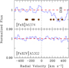 |
Fig. 3 Velocity profiles from stacks of the [Fe X] λ6374.5 and [Fe XIV] λ5302.9 lines from a combined sample of 183/156 VLT/UVES and KECK/HIRES spectra (see Sect. 4.2). The resulting S/N per 20 km s−1 pixel element is 900 for the stacked [Fe X] profile and 1240 for [Fe XIV]. In the profile of the [Fe X] line, a weak DIB is detected near +300 km s−1. The positions of telluric features in the [Fe X] profile are indicated with the crossed circles (from Pettini et al. 1989). Note that the S/N ratios achieved here still are 1–2 orders of magnitude below the values predicted by our models (see Fig. 2). |
5 Outlook
5.1 General prospects from future spectroscopic surveys
While the current archival spectral data base is insufficient to reach the required S/N to obtain meaningful constraints on [Fe X] and [Fe XIV] in the Milky Way’s coronal gas via stacking, the prospects from observational surveys in the near future are excellent. With the advent of several new survey instruments and the installation of extremely sensitve optical telescopes such as the ESO Extremely Large Telescope (ELT; eso.elt.org), there soon will be several millions of spectra available at mediumto high spectral resolution that will open completely new windows to search for extremely weak absorption features of various ions in the foreground gas in the Milky Way’s interstellar and circumgalactic gas (D’Odorico et al. 2024).
Fresco et al. (2020) have explored in detail the prospects of using future spectroscopic surveys to investigate hot gas at ∼107 K around damped Ly α absorbers in the early Universe by stacking a large number of optical spectra. Their goal is to put constraints on the absorption strength of the red-shifted forbidden [Fe XXI] λ1354.1 UV line (Anderson & Sunyaev 2016) in the hot gas around these (proto)galactic structures at median redshift of ⟨zabs⟩ = 2.5. In their paper, the authors discuss the instrumental capabilities of future spectroscopic surveys with millions of optical spectra from projects including i) the Multi-Object Spectrograph Telescope (4MOST), a high-multiplex spectroscopic survey instrument for the 4 m VISTA telescope at ESO (de Jong 2019; Mainieri et al. 2023), for which science operations are expected to start in mid-2026; ii) the WEAVE instrument (Jin et al. 2024), designed for the William Herschel Telescope (WHT), which had first light in Dec 2022; and iii) the AmazoNes high Dispersion Echelle Spectrograph (ANDES; formerly named HIRES), which will be installed on the 39 m Extremely Large Telescope (ELT) currently under construction (Marconi et al. 2022; D’Odorico et al. 2024). For details of these instruments and their performance in the context of stacking experiments, we refer to the discussion in Fresco et al. (2020).
The search for redshifted [Fe XXI] absorption around high-z DLAs, such as that described in Fresco et al. (2020), is not only limited by the number of high-redshift (z > 2.2) background quasars, but also by the cosmological number density (e.g., cross-section) of these absorbers. In contrast, every extragalactic sight line passes the hot coronal gas of the Milky Way, boosting the number of available spectra for stacking experiments using [Fe X] and [Fe XIV] and other weak absorption features in the Galaxy’s CGM and ISM.
Achieving a S/N as high as 25 000 in a spectral stack, as estimated for the [Fe XIV] line in Sect. 4.1, will be extremely challenging, however. Depending on the type of background sources (e.g., AGN, galaxy, star) and their redshift distribution, only a certain fraction of the available spectra can be used for a stack in the [Fe X] and [Fe XIV] wavelength region due to blending effects and continuum issues. For our VLT/UVES sample described in Sect. 4.2, for example, this fraction comes out to 20–25%.
Predictions for detecting [Fe XIV] in future surveys.
In Table 1, we list the minimum number of usable spectra,  , required to reach a S/N of 25 000 per 50 km s−1 wide bin element (second column) as a function of the average S/N per bin in the spectral sample. For a reliable estimate for
  , we need to know the overall sample size of available sources, their exact type and redshift distribution as well as their S/N distribution. The actual S/N achieved from a mix of possible instruments and background sources would also need to be evaluated from a large set of mock spectra with properties similar to those of the real data.
5.2 Example: Potential stacking experiments with 4MOST data
In the following, we elaborate more on the scientific potential of upcoming spectral surveys for [Fe XIV] stacking experiments by focussing on the 4MOST instrument (de Jong 2019). Designed as a high-multiplex spectroscopic survey instrument for the 4 m VISTA telescope at ESO, 4MOST has both a Low-Resolution Spectrograph (LRS; R ≈ 5600 at 5302 Å, corresponding to Δv = 53.5 km s−1) and a High-Resolution Spectrograph (HRS; R ≈ 19 000 at 5302 Å, corresponding to Δv=15.8 km s−1). In principle, the spectral data from both of these instrumental setups therefore can be used for [Fe XIV] stacking experiments. 4MOST is expected to deliver LRS and HRS data for several million extragalactic sources (AGN and galaxies) as part of the Extragalactic Consortium Surveys (e.g., Richards et al. 2019; Merloni et al. 2019) and the Extragalactic Community Surveys (e.g., Bauer et al. 2023; Péroux et al. 2023) covering a broad range of S/N ratios. With such a rich data set, it hopefully will be possible to constrain the mean [Fe XIV] column density in the Milky Way disk and halo and estimate the total amount of million-degree gas in our Galaxy.
As mentioned above, the biggest advantage of using stacked optical spectra compared to X-ray observations and studies of the dispersion measure lies in the (relatively) high spectral and radial-velocity resolution of optical spectrographs (even in their “low-resolution” modes). Also a moderate velocity resolution of Δv ≈ 50 km s−1 will be sufficient to explore the radial velocity profile of the hot gas in and around the Milky Way and to estimate its mass as a function of distance to the Sun.
If sufficient S/N can be achieved even with spectral subsamples, it might also be possible to investigate the patchiness of the hot gas in the Milky Way on angular scales (see Kaaret et al. 2020) and (together with the velocity information) to localize the hot gas reservoirs in the inner and outer Milky Way halo, such as in the disk-halo interface (Savage et al. 2003) and in the extra-planar regions influenced by the Galaxy’s nuclear ouflow (“eROSITA bubbles;” Predehl et al. 2020; Sarkar 2024). Such data could also provide important information on the possible corotation of the hot halo with the underlying disk, as proposed by Hodges-Kluck et al. (2016) based on low-resolution X-ray data.
Because of its relatively large angular extent (Richter et al. 2017, their Fig. 8) and its substantial radial velocity offset from the Milky Way (300 km s−1), also the extended corona of M31 might be a potential target for a [Fe XIV] stacking experiment using extragalactic sight lines in the direction of the Local Group barycenter (see also Lehner et al. 2015, 2020). Such observations also could be coupled to FRB measurements to constrain N(Fe)/N(H) and thus the metallicity of the coronal gas in the Milky Way and M31 haloes.
While 4MOST will also survey hundreds of thousands of LMC and SMC stars and Milky Way halo stars (Cioni et al. 2019; Helmi et al. 2019; Christlieb et al. 2019), it is impossible to forecast their suitability for [Fe XIV] stacking experiments to constrain the hot-gas mass within the inner ∼50 kpc of the Milky Way halo and the hot halo of the Magellanic Clouds (Lucchini et al. 2024) because of the complex stellar continua.
6 Summary and conclusions
In this paper, we explore the possibility of studying the hot coronal gas of the Milky Way at T ≥ 106 K by analyzing the highly forbidden solar coronal lines of [Fe X] and [Fe XIV] in the optical in absorption against bright extragalactic background sources. The main results of our study can be summarized as follows:
- (1)
Using an analytic model of the Milky Way’s coronal gas distribution, results from the HESTIA simulations of the Local Group, and constraints from FRB observations, we predict that the mean hydrogen column density for T ≥ 106 K gas along a typical halo sight line from the Sun to the Galaxy’s virial radius is N(H) ≈ 5 × 1020 cm−2. Assuming the gas to be in a collisional ionization equilibrium and adopting an iron abundance half of the solar value, the expected Fe X and Fe XIV column densities are log N(Fe X) = 15.40 and log N(Fe XIV) = 15.23, where we expect nonthermal gas motions to dominate the Fe X and Fe XIV line widths.
- (2)
Based on the atomic data for the lines of [Fe X] λ6374.5 and [Fe XIV] λ5302.9, we predict characteristic equivalent widths for the coronal gas of W6347=190 μÅ and W5302 = 220 μÅ. We investigated the typical velocity dispersion of the hot gas cells in the HESTIA simulation and used this to generate synthetic absorption profiles for these extremely weak lines with and without noise. We conclude that a minimum S/N of ∼ 50 000 is required to detect [Fe X] λ6374.5 absorption at a 3σ level, while for [Fe XIV] λ5302.9 the required S/N is ∼25 000.
- (3)
We combined archival high-resolution spectral data of 739 AGNs from VLT/UVES and KECK/HIRES to construct a composite spectrum from stacking and to provide upper limits for N(Fe X) and N(Fe XIV) in the Milky Way halo. As expected, we did not find [Fe X] and [Fe XIV] absorption in the stacked spectrum, but we did obtain 3σ upper limits of log N(Fe X) ≤ 16.27 and log N(Fe XIV) ≤ 15.85. Our composite spectrum achieves a S/N ≈ 1240 near 5302 Å and ≈ 900 near 6374 Å. A feature near 6380 Å is clearly evident in the composite spectrum, the measured equivalent width being 29.5 mÅ. We identified this feature as a DIB in the foreground interstellar gas in the Milky Way disk.
- (4)
Finally, we discuss the possibility of detecting [Fe X] and [Fe XIV] absorption using new instruments and ongoing and future observational campaigns. We demonstrate that the upcoming extragalactic spectral surveys with millions of medium- to high-resolution optical spectra will provide an unprecedented wealth of absorption-line data that offers the prospect of detecting the extremely weak [Fe X] and [Fe XIV] lines in the Milky Way’s coronal gas.
Our study implies that future systematic studies of the optical [Fe X] and [Fe XIV] intersystem lines in stacked AGN spectra potentially provide important information on the hot component of the Galaxy’s CGM and the total mass therein. With a somewhat higher oscillator strength, a spectral region that is not undergoing contamination by DIBs and telluric features, and a peak abundance near 2 × 10⁶ K, the [Fe XIV] λ5302.9 line represents the most promising candidate to explore the coronal gas of the Milky Way with the “coronal lines” of iron.
Acknowledgements
This study makes extensive use of the SQUAD and KODIAQ spectral data libraries; we thank M.T. Murphy and J.M. O’Meara for sharing their data with us and providing helpful comments.
References
- Afruni, A., Pezulli, G., Fraternali, F., & Gronnow, A., 2023, MNRAS, 524, 2351 [NASA ADS] [CrossRef] [Google Scholar]
- Anderson, M. E., & Sunyaev, R., 2016, MNRAS, 459, 2806 [Google Scholar]
- Anderson, M. E., & Sunyaev, R., 2018, A&A, 617, A123 [NASA ADS] [CrossRef] [EDP Sciences] [Google Scholar]
- Asplund, M., Grevesse, N., Jacques Sauval, A., & Scott, P., 2009, ARA&A, 47, 481 [NASA ADS] [CrossRef] [Google Scholar]
- Bauer, F. E., Lira, P., Anguita, T., et al. 2023, The Messenger, 190, 34 [NASA ADS] [Google Scholar]
- Ben Bekhti, N., Richter, P., Westmeier, T., & Murphy, M. T., 2008, A&A, 487, 583 [NASA ADS] [CrossRef] [EDP Sciences] [Google Scholar]
- Ben Bekhti, N., Winkel, B., Richter, P., et al. 2012, A&A, 542, A110 [NASA ADS] [CrossRef] [EDP Sciences] [Google Scholar]
- Bhattacharyya, J., Das, S., Gupta, A., Mathur, S., & Korngold, Y., 2023, ApJ, 952, 41 [NASA ADS] [CrossRef] [Google Scholar]
- Biaus, L., Nuza, S. E., Richter, P., et al. 2022, MNRAS, 517, 6170 [Google Scholar]
- Bryans, P., Landi, E., & Savin, D.E., 2009, ApJ, 691, 1540 [CrossRef] [Google Scholar]
- Cioni, M.-R. L., Storm, J., Cameron, P. M., et al. 2019, The Messenger, 175, 54 [NASA ADS] [Google Scholar]
- Crain, R. A., & van de Voort, F., 2023, ARA&A, 61, 473 [NASA ADS] [CrossRef] [Google Scholar]
- Christlieb, N., Battistini, C., Bonifacio, P., et al. 2019, The Messenger, 175, 26 [NASA ADS] [Google Scholar]
- Comparat, J., Truong, N., Merloni, A., et al. 2022, A&A, 666, A156 [NASA ADS] [CrossRef] [EDP Sciences] [Google Scholar]
- Cook, A. M., Bhardwaj, M., Gaensler, B. M., et al. 2023, ApJ, 946, 58 [NASA ADS] [CrossRef] [Google Scholar]
- Damle, M., Sparre, M., Richter, P., et al. 2022, MNRAS, 512, 3717 [CrossRef] [Google Scholar]
- Damle, M., Tonnesen, S., Sparre, M., & Richter, P., 2025, ApJ, 986, 69 [Google Scholar]
- Das, S., Mathur, S., Gupta, A., & Krongold, Y., 2021, ApJ, 918, 83 [NASA ADS] [CrossRef] [Google Scholar]
- de Jong, R. S., 2019, Nat. Astron., 3, 574 [NASA ADS] [CrossRef] [Google Scholar]
- D’Odorico, V., Christiani, S., Pomante, E., et al. 2016, MNRAS, 463, 2690 [Google Scholar]
- D’Odorico, V., Bolton, J. S., Christensen, L., et al. 2024, ExA, 58, 21 [Google Scholar]
- Fang, T., Mckee F. C., Canizares, C. R., & Wolfire, M., 2006, ApJ, 644, 174 [Google Scholar]
- Fontana, A., & Ballester, P., 1995, ESO Messenger, 80, 3 [Google Scholar]
- Fresco, A. Y., Péroux, C., Merloni, A., Hamanowizc, A., & Szakacs, R., 2020, MNRAS, 499, 5230 [NASA ADS] [CrossRef] [Google Scholar]
- Fox, A. J., Richter, P., Wakker, B. P., et al. 2013, ApJ, 772, 111 [Google Scholar]
- Fuhr, J. R., Martin, G. A., & Wiese, W. L., 1988, J. Phys. Chem. Ref. Data, 17, 1 [Google Scholar]
- Gnat, O., & Sternberg, A., 2007, ApJS, 168, 213 [NASA ADS] [CrossRef] [Google Scholar]
- Grand, R. J. J., Gómez, F. A., Marinacci, F., et al. 2017, MNRAS, 467, 179 [NASA ADS] [Google Scholar]
- Grotrian, W., 1939, Naturwissenschaften, 27, 214 [NASA ADS] [CrossRef] [Google Scholar]
- Guber, C. R., & Richter, P., 2016, A&A, 591, A137 [NASA ADS] [CrossRef] [EDP Sciences] [Google Scholar]
- Guber, C. R., Richter, P., & Wendt, M., 2018, A&A, 609, A85 [NASA ADS] [CrossRef] [EDP Sciences] [Google Scholar]
- Hani, M. H., Ellison, S. L., Sparre, M., et al. 2019, MNRAS, 488, 135 [Google Scholar]
- Helmi, A., Irwin, M., Deason, A., et al. 2019, The Messenger, 175, 23 [NASA ADS] [Google Scholar]
- Hobbs, L. M., 1984, ApJ, 280, 132 [Google Scholar]
- Hobbs, L. M., 1985, ApJ, 298, 357 [Google Scholar]
- Hobbs, L.M., & Albert, C. E., 1984, ApJ, 281, 639 [Google Scholar]
- Hobbs, L. M., York, D. G., Snow, T. P., et al. 2008, ApJ, 680, 1256 [NASA ADS] [CrossRef] [Google Scholar]
- Hodges-Kluck, E. J., Miller, M. J., & Bregman, J. N., 2016, ApJ, 822, 21 [NASA ADS] [CrossRef] [Google Scholar]
- Jenniskens, P., & Desert, F.-X., 1994, A&AS, 106, 39 [NASA ADS] [Google Scholar]
- Jin, S., Trager, S. C., & Dalton, G. B., 2024, MNRAS, 530, 2688 [NASA ADS] [CrossRef] [Google Scholar]
- Kaaret, P., Koutroumpa, D., Kuntz, K. D., et al. 2020, Nat. Astron., 4, 1072 [CrossRef] [Google Scholar]
- Klypin, A., Kravtsov, A. V., Bullock, J. S., & Primack J. R., 2001, ApJ, 554, 903 [Google Scholar]
- Kotuš, S. M., Murphy, M. T., & Carswell, R. F., 2017, MNRAS, 464, 3679 [Google Scholar]
- Kramida, A., Ralchenko, Y., Reader, J., & the NIST ASD Team 2023, NIST Atomic Spectra Database, ver. 5.11, online [Google Scholar]
- Krishnarao, D., Fox, A. J., D’Onghia, E., et al. 2022, Nature, 609, 58 [Google Scholar]
- Lan, T.-W., Ménard, B., & Zhu, G., 2015, MNRAS, 452, 3629 [Google Scholar]
- Lehner, N., Savage, B. D., Richter, P., et al. 2007, ApJ, 658, 680 [Google Scholar]
- Lehner, N., Howk, J. C., & Wakker, B. P., 2015, ApJ, 804, 79 [NASA ADS] [CrossRef] [Google Scholar]
- Lehner, N., Berek, S. C., Howk, J. C., et al. 2020, ApJ, 900, 9 [Google Scholar]
- Li, J.-T., & Bregman, J. N. 2017, ApJ, 849, L105 [Google Scholar]
- Liu, W., Chiao, M., Collier, M. R., et al. 2017, ApJ, 83433 [Google Scholar]
- Libeskind, N. I., Carlesi, E., Grand, R. J. J., et al. 2020, MNRAS, 498, 2698 [Google Scholar]
- Locatelli, N., Ponti, G., Zheng, X., et al. 2024, A&A, 681, A78 [NASA ADS] [CrossRef] [EDP Sciences] [Google Scholar]
- Lorimer, D. R., Bailes, M., McLaughlin, M. A., Narkevic, D. J., & Crawford, F., 2007, Science, 318, 777 [Google Scholar]
- Lucchini, S., D’Onghia, E., & Fox, A. J., 2024, ApJ, 967, L16 [Google Scholar]
- Mainieri, V., Leibundgut, B., de Jong, R. S., et al. 2023, The Messenger, 190, 3 [Google Scholar]
- Malaney, R. A., & Clampin, M., 1988, ApJ, 335, L57 [Google Scholar]
- Maller, A. H., & Bullock, J. S., 2004, MNRAS, 355, 694 [CrossRef] [Google Scholar]
- Marasco, A., Fraternali, F., Lehner, N., & Howk, J. C., 2022, MNRAS, 515, 4176 [NASA ADS] [CrossRef] [Google Scholar]
- Marconi, A., Abreu, M., Adibekyan, V., et al. 2022, SPIE, 12184, 24 [Google Scholar]
- Martynenko, N., 2022, MNRAS, 511, 843 [Google Scholar]
- Merloni, A., Alexander, D. A., Banerji, B., et al.,, 2019, The Messenger, 175, 42 [Google Scholar]
- Meyer, D. M., & Lauroesch, J. T., 1999, ApJ, 520, L103 [NASA ADS] [CrossRef] [Google Scholar]
- Miller, M. J., & Bregman, J. N., 2013, ApJ, 770, 118 [NASA ADS] [CrossRef] [Google Scholar]
- Miller, M. J., & Bregman, J. N., 2015, ApJ, 800, 14 [NASA ADS] [CrossRef] [Google Scholar]
- Murga, M., Zhu, G., Ménard, B., & Lan, T.-W. 2015, MNRAS, 452, 511 [NASA ADS] [CrossRef] [Google Scholar]
- Murphy, M. T., Kacprzak, G. G., Savorgnan, G. A. D., & Carswell, R. F., 2019, MNRAS, 482, 3458 [NASA ADS] [CrossRef] [Google Scholar]
- Naab, T., & Ostriker, J. P., 2017, ARA&A, 55, 59 [Google Scholar]
- Navarro, J. F., Frenk, C. S., & White, S. D. M., 1995, MNRAS, 275, 56 [NASA ADS] [CrossRef] [Google Scholar]
- O’Meara, J. M., Lehner, N., Howk, J. C., et al. 2017, AJ, 154, 114 [CrossRef] [Google Scholar]
- Péroux, C., & Howk, J. C., 2020, ARA&A, 58, 363 [CrossRef] [Google Scholar]
- Péroux, C., Merloni, A., Liske, J., et al. 2023, The Messenger, 190, 42 [NASA ADS] [Google Scholar]
- Pettini, M., & D’Odorico, S., 1986, ApJ, 310, 700 [Google Scholar]
- Pettini, M., Stathakis, R., D’Odorico, S., Molaro, P., & Vladilo, G., 1989, ApJ, 340, 256 [Google Scholar]
- Predehl, P., Sunyaev, R. A., Becker, W., et al. 2020, Nature, 588, 277 [Google Scholar]
- Prochaska, J. X., & Zheng, Y., 2019, MNRAS, 485, 648 [NASA ADS] [Google Scholar]
- Putman, M. E., Staveley-Smith, L., Freeman, K. C., et al. 2003, ApJ, 586, 170 [NASA ADS] [CrossRef] [Google Scholar]
- Richter, P., 2012, ApJ, 750, 165 [Google Scholar]
- Richter, P., 2017, ASSL, 430, 15 [Google Scholar]
- Richter, P., 2020, ApJ, 892, 33 [Google Scholar]
- Richard, J., Kneib, J.-P., Blake, C., et al. 2019, The Messenger, 175, 50 [NASA ADS] [Google Scholar]
- Richter, P., Savage, B. D., Wakker, B. P., Sembach, K. R., & Kalberla, P. M. W., 2001, ApJ, 549, 281 [Google Scholar]
- Richter, P., Sembach, K. R., & Howk, J. C., 2003, A&A, 405, 1013 [NASA ADS] [CrossRef] [EDP Sciences] [Google Scholar]
- Richter, P., Westmeier, T., & Brüns, C., 2005, A&A, 442, L49 [NASA ADS] [CrossRef] [EDP Sciences] [Google Scholar]
- Richter, P., Savage, B. D., Sembach, K. R., & Tripp, T. M. 2006a, A&A, 445, 827 [NASA ADS] [CrossRef] [EDP Sciences] [Google Scholar]
- Richter, P., Fang, T., & Bryan, G. L. 2006b, A&A, 451, 767 [NASA ADS] [CrossRef] [EDP Sciences] [Google Scholar]
- Richter, P., Krause, F., Fechner, C., Charlton, J. C., & Murphy, M. T., 2011, A&A, 528, A12 [NASA ADS] [CrossRef] [EDP Sciences] [Google Scholar]
- Richter, P., Fox, A. J., Wakker, B. P., et al. 2013, ApJ, 772, 111 [Google Scholar]
- Richter, P., Fox, A. J., Ben Bekhti, N., et al. 2014, AN, 335, 92 [Google Scholar]
- Richter, P., Nuza, S. E., Fox, A. J., et al. 2017, A&A, 607, A48 [NASA ADS] [CrossRef] [EDP Sciences] [Google Scholar]
- Rünger, F., Sparre, M., Richter, P., et al. 2025, A&A, 700, A131 [NASA ADS] [CrossRef] [EDP Sciences] [Google Scholar]
- Sarkar, K. C., 2024, A&ARv, 32, 1 [NASA ADS] [CrossRef] [Google Scholar]
- Savage, B. D., Sembach, K. R., Wakker, B. P., et al. 2003, ApJS, 146, 125 [Google Scholar]
- Sembach, K. R., Wakker, B. P., Savage, B. D., et al. 2003, ApJS, 146, 165 [CrossRef] [Google Scholar]
- Shirai, T., Sugar, J., Musgrove, A., & Wiese, W. L., 2000, J. Phys. Chem. Ref. Data, Monograph, 8 [Google Scholar]
- SpitzerJr., L., 1956, ApJ, 124, 20 [NASA ADS] [CrossRef] [Google Scholar]
- Springel, V., 2010, MNRAS, 401, 791 [Google Scholar]
- Sutherland, R. S., & Dopita, M. A., 1993, ApJS, 88, 253 [Google Scholar]
- Tepper-García, T., Richter, P., Schaye, J., et al. 2012, MNRAS, 425, 1640 [Google Scholar]
- Tepper-García, T., Richter, P., & Schaye, J., 2014, MNRAS, 436, 2036 [Google Scholar]
- Tripp, T. M., Sembach, K. R., Bowen, D. V., et al. 2008, ApJ, 177, 39 [Google Scholar]
- Tumlinson, J., Peeples, M. S., & Werk, J. K., 2017, ARA&A, 55, 389 [Google Scholar]
- Wampler, E. J., Chen, J. S., & Setti, G., 1991, A&A, 248, 633 [Google Scholar]
- Wang, Q., Hamilton, T., & Helfand, D. J., 1989, Nature, 341, 309 [Google Scholar]
- White, S. D. M., & Frenk, C. S., 1991, ApJ, 379, 52 [Google Scholar]
- York, D. G., & Cowie, L. L., 1983, ApJ, 264, 49 [Google Scholar]
- Zastrocky, T. W., Howk, J. C., Lehner, N., & O’Meara, J. M., 2018, AARN, 2, 227 [Google Scholar]
Throughout this paper, we provide air-wavelengths in units Å for the optical transitions of [Fe X] and [Fe XIV], as given in the NIST Atomic Spectra Database (Kramida et al. 2023), while we give vacuum wavelengths for transitions of UV lines at λ≤ 3000 Å.
All Tables
All Figures
|
Fig. 1 Fractional abundances of Fe+9 and Fe+13 in a collisional ionization equilibrium (from Bryans et al. 2009, see also Sect. 2.1). |
| In the text | |
|
Fig. 2 Synthetic spectra of the [Fe X] at λ6374.5 and [Fe XIV] λ5302.9 lines from our halo model described in Sect. 4.1. The upper two panels show the noise-free absorption profiles, the lower two panels show the profiles with the minimum S/N required for a 3σ detection, as given in the lower left corners. The spectra are generated using a spectral resolution of R = 45 000 and a sampling of 1.5 pixels per resolution element. |
| In the text | |
|
Fig. 3 Velocity profiles from stacks of the [Fe X] λ6374.5 and [Fe XIV] λ5302.9 lines from a combined sample of 183/156 VLT/UVES and KECK/HIRES spectra (see Sect. 4.2). The resulting S/N per 20 km s−1 pixel element is 900 for the stacked [Fe X] profile and 1240 for [Fe XIV]. In the profile of the [Fe X] line, a weak DIB is detected near +300 km s−1. The positions of telluric features in the [Fe X] profile are indicated with the crossed circles (from Pettini et al. 1989). Note that the S/N ratios achieved here still are 1–2 orders of magnitude below the values predicted by our models (see Fig. 2). |
| In the text | |
Current usage metrics show cumulative count of Article Views (full-text article views including HTML views, PDF and ePub downloads, according to the available data) and Abstracts Views on Vision4Press platform.
Data correspond to usage on the plateform after 2015. The current usage metrics is available 48-96 hours after online publication and is updated daily on week days.
Initial download of the metrics may take a while.