| Issue |
A&A
Volume 701, September 2025
|
|
|---|---|---|
| Article Number | A257 | |
| Number of page(s) | 6 | |
| Section | Stellar structure and evolution | |
| DOI | https://doi.org/10.1051/0004-6361/202556349 | |
| Published online | 19 September 2025 | |
Characterising the red giant companion of the black hole in the BH2 system
Robust determination of the fundamental parameters
1
Dipartimento di Fisica “Enrico Fermi”, Università di Pisa, Largo Pontecorvo 3, I-56127 Pisa, Italy
2
INFN, Sezione di Pisa, Largo Pontecorvo 3, I-56127 Pisa, Italy
⋆ Corresponding author.
Received:
10
July
2025
Accepted:
21
August
2025
Abstract
Context. The recently discovered Gaia BH2 binary system composed of a red giant star and a dormant black hole offers a great opportunity to investigate the formation of binary black holes.
Aims. From this perspective, we performed an independent determination of fundamental parameters of the luminous giant star BH2*, a young thin disk object and high [α/Fe]. A peculiarity of our investigation is the adoption of stellar models specifically tailored to Galactic red giant branch stars with chemical abundances and [α/Fe] scaling calibrated over a large sample of objects.
Methods. We derived the estimated system parameters using the SCEPtER pipeline, which relies on spectroscopic and global asteroseismic constraints from literature investigations and utilises a large grid of stellar models. We explored the robustness of the determination by adopting two different corrections for Δν values from the literature to account for the current uncertainty on this quantity.
Results. The estimated masses ranged from M = 1.19 ± 0.05 M⊙ to M = 1.26 ± 0.05 M⊙. The global age of the system was determined to be 4.8 ± 0.5 (sys) ± 0.7 (rand) Gyr. These estimates are consistent with recent findings but exhibit a significantly reduced uncertainty. The radius of BH2* was estimated to be between 8.23 ± 0.12 and 8.47 ± 0.13 R⊙. To explore potential merging or accretion events in the evolutionary history of BH2*, we conducted a supplementary radius estimation based on surface brightness–colour relations utilising V and K magnitudes along with Gaia DR3 parallax data. This estimate, based on two validated relations, indicated a significantly lower radius range of 7.50 ± 0.23 to 7.80 ± 0.23 R⊙. However, this discrepancy was not large enough to rule out a mere fluctuation. Finally, we explored the possibility of inferring non-single-star evolutionary scenarios for BH2* based on its chemical abundance pattern. Principal component analysis (PCA) using α-element abundances and sodium revealed that the position of BH2* in the PCA space was extreme, even when compared to other young α-enhanced stars identified as suspect merging products.
Conclusions. Further asteroseismic observations and carbon and nitrogen determinations would enable a more detailed characterisation of BH2* and provide further insights into its evolutionary history.
Key words: methods: statistical / stars: black holes / stars: evolution / stars: fundamental parameters / stars: interiors / Galaxy: abundances
© The Authors 2025
 Open Access article, published by EDP Sciences, under the terms of the Creative Commons Attribution License (https://creativecommons.org/licenses/by/4.0), which permits unrestricted use, distribution, and reproduction in any medium, provided the original work is properly cited.
This article is published in open access under the Subscribe to Open model. This email address is being protected from spambots. You need JavaScript enabled to view it. to support open access publication.
1. Introduction
The recent identification of Gaia BH2, a binary system composed of a red giant star and a dormant black hole (El-Badry et al. 2023; Gaia Collaboration 2024), and the subsequent asteroseismic characterisation of the luminous component (hereafter BH2*) by Hey et al. (2025) have offered an opportunity to investigate binary black hole formation (see e.g. Gilkis & Mazeh 2024; Li et al. 2024; Tanikawa et al. 2024). Moreover, the knowledge of the fundamental parameters – such as the metallicity, mass, and age – of the luminous component offers the opportunity to infer those of the non-luminous component, which are not directly measurable.
The spectroscopic investigation by El-Badry et al. (2023) characterised the luminous component as a red giant branch (RGB) star, with Teff = 4604 ± 87 K, a noticeable α enhancement [α/Fe] = 0.26 ± 0.05, and sub-solar metallicity [Fe/H] = −0.22 ± 0.02. The distance of the system based on the Gaia DR3 non-single object table parallax is d = 1.16 ± 0.02 kpc. The analysis of El-Badry et al. (2023) suggests a primordial origin of the α-enhancement of BH2* mainly because of the wide orbit of the system. However, they did not definitively rule out a possible pollution of low-velocity ejecta during a failed supernova. Moreover, they found that the galactocentric orbit of the system is typical of thin discs. From a fit of the broad-band spectral energy distribution obtained by combining the Swift UVM2 magnitude, synthetic SDSS ugriz photometry constructed from Gaia BP/RP spectra, 2MASS JHK photometry, and WISE W1 W2 W3 photometry, El-Badry et al. (2023) inferred the temperature and radius of the red giant as Teff = 4615 K, which is nearly identical to the spectroscopic determination, and R = 7.77 ± 0.25 R⊙. The mass of the star, estimated from MIST tracks (Choi et al. 2016), was fixed at M = 1.07 ± 0.19 M⊙.
These data were further revised by Hey et al. (2025) following a successful asteroseismic analysis of the Transiting Exoplanet Survey Satellite (TESS) light curve. By using the PySYD pipeline, they determined the global asteroseismic parameters, that is, the maximum power excess (νmax = 60.15 ± 0.57 μHz) and the large frequency separation (Δν = 5.99 ± 0.03 μHz) for BH2*, with a noticeable precision of 1% in νmax and 0.5% in Δν. The asteroseismic pipeline solar reference values are νmax, ⊙ = 3090 μHz, Δν⊙ = 135.1 μHz and Teff, ⊙ = 5777 K. The asteroseismic parameters were then adopted to infer the mass and the radius of the star from corrected asteroseismic scaling relations (Ulrich 1986; Kjeldsen et al. 2005) utilising asfgrid software (Sharma et al. 2016; Stello & Sharma 2022). Given the fact that the grid of models adopted in that investigation does not account for α enhancement, they adopted the commonly used Salaris et al. (1993) scaling law to obtain [M/H] = −0.037 ± 0.04 dex from [Fe/H] and [α/Fe]. The fundamental parameters for BH2* were estimated as M = 1.23 ± 0.09 M⊙ and  . The age of the star, inferred from the cnfgiant grid, available in MODELFLOWS (Hon et al. 2024), was
  Gyr.
Gyr.
The robustness of these determinations depends chiefly on the basic assumption of reliability of the stellar models adopted for the estimation. Recently Valle et al. (2024a) discussed the importance of adopting a grid of stellar models that matches the observed [α/Fe] when estimating field star characteristics. The study was expanded in Valle et al. (2024b) by their investigation of the chemical composition of giant stars in the APO-K2 catalogue (Schonhut-Stasik et al. 2024). Their research highlights a global difference in the scaling of α element abundances with [α/Fe], contrary to what is usually assumed in stellar model grids. By adopting empirically calibrated dependences, Valle et al. (2024c) estimated the age of the APO-K2 RGB stars, reporting on a likely cancellation that mitigated the effect of adopting the correct empirical trend for each element with respect to the uniform one. This fortunate cancellation, however, depends on the recalibration of the effective temperature constraint. In fact, for RGB stars, the use of effective temperature as a constraint in fitting procedures is problematic due to substantial observational and theoretical uncertainties (e.g. Martig et al. 2015; Warfield et al. 2021; Vincenzo et al. 2021). Discrepancies between model and observed temperatures can significantly bias age estimates, as they directly influence mass determination, a key parameter in age calculations. This effect, explored in detail in Valle et al. (2024c), was found to be of fundamental importance for high [α/Fe] stars.
The first aim of this paper is therefore to provide independent estimates of the fundamental parameters of BH2* based on the present empirically calibrated stellar model grid and following the procedure illustrated in Valle et al. (2024c). We also investigate the peculiarity of the chemical composition of BH2* by comparing it with those from the APO-K2 RGB sample. The second aim of this paper is to investigate the reliability of the obtained parameters, and we adopted independent estimates of the stellar radius to do so. We note that surface brightness–colour relations (SBCRs) provide an efficient alternative for determining stellar angular diameters from photometric measurements and parallax. Valle et al. (2024d, 2025) have recently shown the global consistency of giant star radii determined by SBCRs and asteroseismic scaling relations from Kepler and K2 data. It is therefore interesting to compare results from the two methods for BH2* to explore possible discrepancies.
2. Methods
2.1. Observational data and stellar models grid
For the purpose of system characterisation, we adopted both classical atmospheric (Teff, [Fe/H], [α/Fe]) and asteroseismic (Δν, νmax) constraints. The first set is derived from El-Badry et al. (2023), and the second is from Hey et al. (2025). The adopted parameters are summarised in Table 1.
Observational data for the BH2* giant star.
For our fitting procedure, we employed the same stellar model grid as in Valle et al. (2024c); we summarise its key features here. The models cover a mass range of 0.8 to 1.9 M⊙, extending to the RGB tip. The initial metallicity, [Fe/H], varied from −1.5 to 0.4 dex, with a step size of 0.025 dex. We adopted the solar heavy-element mixture from Asplund et al. (2009) as a baseline. The initial helium abundance was determined using the linear relation  , with the primordial helium abundance Yp = 0.2471 from Planck Collaboration VI (2020). The helium-to-metal enrichment ratio, ΔY/ΔZ, was set to 2.0. The α-element enhancement was included for both α elements and aluminium. The models were computed for [α/Fe], ranging from 0.0 to 0.4 dex with a step of 0.1 dex. No convective core overshooting was considered in the computations. This choice was validated a posteriori because the inferred stellar mass is in a range where the effect of this input is negligible (e.g. Claret & Torres 2016, 2017).
A notable aspect of our study is the adoption of non-constant scaling for different α elements. Their dependence on [α/Fe] was derived from the analysis of giant star abundances in the APO-K2 catalogue (Schonhut-Stasik et al. 2024). This analysis, detailed in Valle et al. (2024b), revealed significant variations among elements, most notably a steeper increase in the oxygen abundance relative to other α elements with increasing [α/Fe]. This observation aligns with previous studies (e.g. Bensby et al. 2005; Nissen et al. 2014; Bertran de Lis et al. 2015; Amarsi et al. 2019). Given these discrepancies, ages derived from comparisons with stellar models that do not account for this feature should be interpreted with caution (e.g. VandenBerg et al. 2012; Sun et al. 2023a,b; Valle et al. 2024c). For details regarding other model grid characteristics, such as boundary conditions, mixing-length calibration, radiative opacities, and the reduction process, we refer the reader to Valle et al. (2024c).
2.2. Effective temperature discrepancies
The recent literature highlights the difficulty of adopting the effective temperature as a constraint in fitting procedures for RGB stars due to substantial observational and theoretical uncertainties (e.g. Martig et al. 2015; Warfield et al. 2021; Vincenzo et al. 2021; Valle et al. 2024c). However, neglecting the Teff constraint in the fit is not advisable because in its absence, grid-based estimates for RGB stars are affected by large uncertainties (Pinsonneault et al. 2018). Recent studies have addressed this issue by employing the masses derived from corrected asteroseismic scaling relations as a constraint (Martig et al. 2015; Warfield et al. 2021, 2024), thus mitigating the reliance on effective temperature as a direct observational constraint. We adopted a similar approach, as previously implemented in Valle et al. (2024c).
In detail, we adopted as a constraint the effective temperature estimated by linearly interpolating over the grid of stellar models. The interpolation was carried out in mass, νmax, [α/Fe], and [Fe/H]. The stellar masses used in the process were estimates from corrected asteroseismic scaling relations:
 (1)
(1)
Here, fΔν is a correction factor necessary to reconcile the asteroseismic predictions to directly constrained values of masses and radii. These corrections have been investigated by many authors in different ranges of mass, metallicity, and evolutionary phase (e.g. White et al. 2011; Sharma et al. 2016; Rodrigues et al. 2017; Guggenberger et al. 2017; Li et al. 2022, 2023; Pinsonneault et al. 2025). Including correction factors, the estimated masses and radii reached a general agreement for stars in eclipsing binary systems (e.g. Brogaard et al. 2018; Hekker 2020, and references therein). Currently, correction factor variations of up to 2% are reported in the literature (see e.g. Li et al. 2023; Pinsonneault et al. 2025). We therefore performed our investigation assuming two alternative corrections: those by Sharma et al. (2016) and Stello & Sharma (2022) and those by Li et al. (2023).
The Sharma et al. (2016) correction factor, fΔν, S, was obtained using the asfgrid v0.0.6 software1, resulting in fΔν, s = 0.971. The Li et al. (2023) correction was implemented using the code provided with that paper2, resulting in fΔν, L = 0.958. For the Sharma et al. (2016) corrections, we obtained a stellar mass of MS = 1.207 M⊙ and a corresponding effective temperature in the grid of Teff, S = 4721 K. In the following, we refer to these parameters as scenario S. For the Li et al. (2023) correction (scenario L), we obtained ML = 1.145 M⊙ and Teff, L = 4702 K. The finding of stellar models hotter by about 100 K with respect to observation around [α/Fe] = 0.26 and [Fe/H] = −0.22 agrees with the analysis presented in Valle et al. (2024c).
2.3. Stellar parameter fitting technique
Our analysis was carried out adopting the SCEPtER pipeline3, a well-tested technique for fitting single and binary systems (e.g. Valle et al. 2014, 2015, 2023). The pipeline estimates the stellar age by adopting a grid maximum likelihood approach, relying on the observed quantities o ≡ {Teff, [Fe/H], Δν, νmax}. For every j-th point in the fitting grid, a likelihood estimate is obtained:
 (2)
(2)
 (3)
(3)
Here, oi are the n observational constraints, gij are the j-th grid point corresponding values, and σi are the observational uncertainties. The estimated stellar parameters were obtained by averaging those of all the models with a likelihood greater than 0.95 × Lmax4. The confidence interval for these estimates was obtained by means of a Monte Carlo simulation. We repeated the estimation over a generated sample of size n = 2000. These synthetic stars were obtained by means of Gaussian perturbations around their observed values adopting a diagonal covariance matrix Σ = diag(σ2). The value of [α/Fe] was also perturbed in the same way, and for every iteration, the fitting grid was computed ‘on the fly’ by interpolating the available grids at the specific [α/Fe] value. Given the Gaussian-like shape of the posteriors, the mean of the n masses, radii, and ages were taken as the best estimate of the true values; the standard deviations of the n values were adopted as 1σ confidence intervals.
2.4. SBCRs radius estimation
The SBCRs provide an efficient alternative for determining stellar angular diameters from photometric measurements. The surface brightness, Sλ, of a star is linked to its limb-darkened angular diameter, θ, and its apparent magnitude corrected for the extinction, mλ0. In the V band, SV is defined as
 (4)
(4)
where V0 is the V-band magnitude corrected for extinction. It follows from Eq. (4) that
 (5)
(5)
 (6)
(6)
where d is the heliocentric distance of the star and r is an estimate of the stellar linear radius.
Valle et al. (2024d, 2025) found a noticeable agreement between SBCRs and asteroseismically estimated radii for APO-K2 and end-of-mission Kepler samples. The two techniques rely on different observables and assumptions; therefore, it is interesting to investigate their agreement for BH2*. For this purpose, we adopted two different SBCRs. The first, proposed by Pietrzyński et al. (2019), was
![Mathematical equation: $$ \begin{aligned} {S\!}_V^a = 1.330 [(V - K)_0 - 2.405] + 5.869 \; \mathrm{mag}, \end{aligned} $$](/articles/aa/full_html/2025/09/aa56349-25/aa56349-25-eq10.gif) (7)
(7)
where (V − K)0 is the colour corrected for the reddening. This relation was fitted in the range 2.0 < (V − K)0 < 2.8 mag. The second adopted SBCR was proposed by Salsi et al. (2021):
 (8)
(8)
This relation (from Table 5 in Salsi et al. 2021 for stars of the spectral class F5/K7-II/III) is valid in the range 1.8 < (V − K)0 < 3.9 mag.
To obtain V- and Ks-band magnitudes, we cross-matched the BH2 data with the TESS Input Catalog v8.2. Extinction in the V band AV = 0.58 mag, corresponding to E(B − V)≈0.2, was taken from El-Badry et al. (2023), who obtained it from the 3D dust map by Lallement et al. (2022). The extinction in the K band was estimated from Cardelli et al. (1989) as AK = 0.114 AV.
3. Grid-based and SBCRs stellar parameter estimates
The results of the grid-based fits are presented in Table 2 and in Fig. 1. In both scenarios, the grid-based mass estimates are approximately 0.05 M⊙ higher than those derived from corrected scaling relations. For scenario S, the mass and radius estimates agree with those of Hey et al. (2025), who adopted a Monte Carlo method to derive from asfgridM = 1.23 ± 0.09 M⊙ and  . However, our age estimate 4.3 ± 0.6 Gyr is about 20% lower than the
  Gyr reported in that paper for their asfgrid fit. Despite this difference, the two age determinations remain consistent within their respective uncertainties. Notably, our grid-based modelling yields uncertainties that are nearly half of those of Hey et al. (2025).
Grid-based estimates of age, mass, and radius for BH2*.
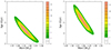 |
Fig. 1. Bi-dimensional kernel density estimators of the joint mass-age distributions. Left: Results obtained using the correction factors from Sharma et al. (2016). Right: Same as in the left panel but using the Li et al. (2023) correction factor. |
In scenario L, we observed lower mass and radius estimates, but these remain consistent with scenario S within the error margins. The age estimate for scenario L is 5.3 ± 0.8 Gyr, which is closer to the determination by Hey et al. (2025) but with a significantly reduced uncertainty. Combining both scenarios, we obtained an age estimate of 4.8 ± 0.5 (sys) ± 0.7 (rand) Gyr.
Radius determinations using SBCRs yielded RP = 7.80 ± 0.23 R⊙ from Pietrzyński et al. (2019) and RS = 7.50 ± 0.23 R⊙ from Salsi et al. (2021), respectively. These SBCR radii are significantly lower than the asteroseismic radii and are inconsistent within their quoted uncertainties. Notably, they are close to the stellar radius estimated from a spectral energy distribution fitting by El-Badry et al. (2023), which is 7.77 ± 0.25 R⊙. The discrepancy of approximately 10% between the SBCR and asteroseismic radii is not sufficient to definitively rule out a random fluctuation. For stars at the distance of BH2*, Valle et al. (2024d) suggest a standard deviation of about 8% between these two techniques. It is crucial to note that the parallax of BH2* was derived from the Gaia non-single star table, nss_two_body_orbit. As discussed in El-Badry et al. (2023), this parallax value was not corrected for zero-point errors, as such corrections are not yet available for non-single star astrometric solutions. Consequently, the potential presence of a hidden systematic error in the SBCR radii cannot be excluded.
4. Element abundances analysis
The analysis presented in the previous section supports the Hey et al. (2025) conclusion that BH2* is part of the young α-enhanced population of Galactic stars. This population has been found to represent about 6% to 10% of thick disc stars (Warfield et al. 2024; Valle et al. 2024c). Hey et al. (2025) discussed the possibility that this high α abundance is due to accretion or merging events and highlighted that the asteroseismic analysis of longer light curves may solve the problem by determining the spacing of the dipole g-mode period, ΔΠ1. This will allow the positioning of BH2* in the ΔΠ1 − Δν diagram to be inspected in order to detect possible anomalies with respect to a single star.
Another possibility to explore an anomalous evolutionary history is offered by the element abundance analysis. The analysis of Valle et al. (2024c) of the [C/N] ratio for the young α-rich thick disc population supports the possible origin of these stars as a result of mergers or mass transfer events. A star-by-star comparison revealed a much higher [C/N] median difference between observations and models in the high-α young population compared to the high-α old group. This discrepancy is often attributed to mergers or mass transfer events between two lower-mass giants, which have preserved their original [C/N] values (Chiappini et al. 2015; Jofré et al. 2016; Grisoni et al. 2024). The importance of assessing the possibility of mass transfer is obvious because this scenario invalidates the age estimate obtained assuming single star evolution.
Unfortunately, neither carbon nor nitrogen abundances were measured in the spectroscopic analysis conducted by El-Badry et al. (2023), making it impossible to directly evaluate the ratio. However, the spectroscopic analysis allowed for the determination of several α element abundances and sodium, making a multivariate comparison with analogous abundances for RGB stars in the APO-K2 catalogue possible. This comparison allowed us to explore the similarity of the chemical composition of BH2* with those of the young α-enhanced stars identified in Valle et al. (2024c).
For this purpose, the abundances [O/Fe], [Na/Fe], [Mg/Fe], [Al/Fe], [Si/Fe], [Ca/Fe], and [Ti/Fe] were extracted for the stars in the APO-K2 catalogue. A principal component analysis (Venables & Ripley 2002; Feigelson & Babu 2012) was performed to reduce the dimensionality of the sample. The technique achieves this reduction by transforming the original variables – i.e. the observed abundances – into a new set called principal components, which are linear combinations of the original ones. These principal components are ordered on the basis of the amount of variance they explain, with the first few capturing the most significant information. The first two components, PCA1 and PCA2, which explain 90% of the total variance, were adopted to plot the APO-K2 data set in Fig. 2. In this plot, young α-enhanced stars with [(C+N+O)/Fe] greater than 0.18 and mass greater than 1.2 M⊙ were identified by larger symbols. These stars probably experienced a merging or accretion event during their evolution (Chiappini et al. 2015; Jofré et al. 2016; Grisoni et al. 2024; Valle et al. 2024c).
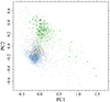 |
Fig. 2. Principal component analysis for the abundances of stars in the APO-K2 catalogue and BH2*. Blue and green points correspond, respectively, to the α-poor and α-rich populations – generally identified by thin and thick disc components. Red points identify transition stars not unambiguously classified in the two previous groups (see Schonhut-Stasik et al. 2024, for details about the classification). Larger symbols identify young α-rich stars (see text). The position of BH2* is marked by a purple square. |
Based on the same element abundances, the position of BH2* in the principal component space was calculated. Figure 2 clearly shows the significant anomalous composition of BH2* with respect to thin disc stars. Its position in the plot is extreme, even for the young α-rich population. Although the anomalous BH2* position in the PCA space might suggest a non-standard evolution of the red giant’s progenitor, the lack of reliable carbon and nitrogen abundance determinations precludes rigorous and definitive conclusions.
A possible explanation for such an abundance pattern is pollution from the black hole progenitor’s supernova ejecta. This scenario, where α element enhancement results from the accretion of supernova material, has been proposed for other X-ray binaries. For instance, Israelian et al. (1999) suggested it for GRO J1655−40, though this was later challenged by Foellmi et al. (2007). Similarly, González Hernández et al. (2011) and Suárez-Andrés et al. (2015) explored it for V404 Cyg and Cygnus X-2, respectively. However, the large orbital separation in the BH2 system makes this direct supernova pollution scenario unlikely. The vast distance between the stars means that most of the supernova ejecta would have dispersed, leading to a negligible modification of the companion star’s surface abundances (El-Badry et al. 2023). Although it is theoretically possible for low-velocity ejecta to be re-accreted by the giant star, thereby altering its α element abundances, this mechanism is highly dependent on the precise energetics of the supernova explosion, and detailed computations are currently lacking to support it (El-Badry et al. 2023). Moreover, the supernova accretion scenario is further disfavoured by the analysis of s-process and r-process element abundances in BH2*. These elements do not display the characteristic signature of supernova enrichment, contradicting what would be expected if significant ejecta accretion had occurred. The observed α enhancement, age estimate, and rapid rotation of BH2* seems to suggest a potential merging or planet engulfment event (Hey et al. 2025), although the current data do not permit a definitive conclusion.
5. Conclusions
We have conducted an independent analysis of the Gaia BH2 system to assess the robustness of the fundamental parameters of the luminous RGB star BH2*. Accurate determination of these parameters is crucial for constraining those of the non-luminous companion. Our analysis builds on previous work. El-Badry et al. (2023) provided spectroscopic constraints, revealing BH2* to be a thin-disc sub-solar metallicity α-enhanced star with [Fe/H] = −0.22 and [α/Fe] = 0.26. Furthermore, Hey et al. (2025) successfully analysed the TESS light curve, yielding global asteroseismic parameters, Δν and νmax.
A key distinction from previous analyses is our utilisation of a stellar model grid specifically calibrated to the elemental abundances of Galactic giant stars from the APO-K2 catalogue (Schonhut-Stasik et al. 2024), as developed by Valle et al. (2024b). The importance of employing a precise link between elemental abundances and [α/Fe] has previously been highlighted by Valle et al. (2024c).
Given the current uncertainty of about 2% in the correction factor for asteroseismic scaling relations in the RGB phase (e.g. Li et al. 2023; Pinsonneault et al. 2025), we have presented two characterisations of BH2*. Using the correction by Sharma et al. (2016), we derived M = 1.26 ± 0.05 M⊙, R = 8.47 ± 0.13 R⊙, and τ = 4.3 ± 0.6. In contrast, with the Li et al. (2023) correction, we obtained M = 1.19 ± 0.05 M⊙, R = 8.23 ± 0.12 R⊙, and τ = 5.3 ± 0.8 Gyr. Both mass and radius estimates are consistent with those reported by Hey et al. (2025), while we report a slightly younger age. Compared to previous determinations, our analysis enables a significant reduction in uncertainties for all parameters. In conclusion, we corroborate that BH2* belongs to the Galactic young α-enhanced population.
To investigate possible merging or accretion events in the evolutionary history of BH2*, as previously hypothesised by El-Badry et al. (2023) and Hey et al. (2025), we performed a supplementary radius estimation using SBCRs. This method has demonstrated competitiveness with asteroseismic estimates for giants in the APO-K2 and Kepler end-of-mission catalogues (Valle et al. 2024d, 2025). Using the SBCRs of Pietrzyński et al. (2019) and Salsi et al. (2021), we obtained reduced radius estimates of 7.80 ± 0.23 R⊙ and 7.50 ± 0.23 R⊙, respectively. Although these SBCR-derived radii are inconsistent with the asteroseismic radii within their respective error bars, the observed 10% discrepancy is not sufficient to definitively exclude a mere fluctuation, considering the 8% variability estimated by Valle et al. (2024d) for objects with parallaxes similar to thatof BH2*.
Finally, we investigated the potential for inferring non-single star evolutionary scenarios for BH2* from its chemical abundance pattern. As shown by Valle et al. (2024c), the [C/N] ratio serves as a powerful tracer of such events in α-enhanced young thick disc stars, consistent with previous literature (Chiappini et al. 2015; Jofré et al. 2016; Grisoni et al. 2024). Due to the absence of carbon and nitrogen abundance determinations, we analysed the global pattern of α elements and sodium, comparing it with that of APO-K2 RGB stars. Principal component analysis revealed an anomalous position for BH2*, exhibiting an extreme composition even compared to other young α-enhanced stars, which are already recognised as likely products of merger events. Future asteroseismic investigations, as envisioned by Hey et al. (2025), utilising longer light curve observations may enable a more detailed characterisation of the interior of BH2*, providing further insights into its evolutionary history.
Publicly available on CRAN: http://CRAN.R-project.org/package=SCEPtER
The likelihood threshold was set for computational efficiency. Negligible differences arose when using a weighted mean where the weight of each model reflects its likelihood.
Acknowledgments
G.V., P.G.P.M. and S.D. acknowledge INFN (Iniziativa specifica TAsP) and support from PRIN MIUR2022 Progetto “CHRONOS” (PI: S. Cassisi) finanziato dall’Unione Europea – Next Generation EU.
References
- Amarsi, A. M., Nissen, P. E., & Skúladóttir, Á. 2019, A&A, 630, A104 [NASA ADS] [CrossRef] [EDP Sciences] [Google Scholar]
- Asplund, M., Grevesse, N., Sauval, A. J., & Scott, P. 2009, ARA&A, 47, 481 [NASA ADS] [CrossRef] [Google Scholar]
- Bensby, T., Feltzing, S., Lundström, I., & Ilyin, I. 2005, A&A, 433, 185 [NASA ADS] [CrossRef] [EDP Sciences] [Google Scholar]
- Bertran de Lis, S., Delgado Mena, E., Adibekyan, V. Z., Santos, N. C., & Sousa, S. G. 2015, A&A, 576, A89 [NASA ADS] [CrossRef] [EDP Sciences] [Google Scholar]
- Brogaard, K., Hansen, C. J., Miglio, A., et al. 2018, MNRAS, 476, 3729 [Google Scholar]
- Cardelli, J. A., Clayton, G. C., & Mathis, J. S. 1989, ApJ, 345, 245 [Google Scholar]
- Chiappini, C., Anders, F., Rodrigues, T. S., et al. 2015, A&A, 576, L12 [NASA ADS] [CrossRef] [EDP Sciences] [Google Scholar]
- Choi, J., Dotter, A., Conroy, C., et al. 2016, ApJ, 823, 102 [Google Scholar]
- Claret, A., & Torres, G. 2016, A&A, 592, A15 [NASA ADS] [CrossRef] [EDP Sciences] [Google Scholar]
- Claret, A., & Torres, G. 2017, ApJ, 849, 18 [Google Scholar]
- El-Badry, K., Rix, H.-W., Cendes, Y., et al. 2023, MNRAS, 521, 4323 [NASA ADS] [CrossRef] [Google Scholar]
- Feigelson, E. D., & Babu, G. J. 2012, Modern Statistical Methods for Astronomy with R Applications (Cambridge: Cambridge University Press) [Google Scholar]
- Foellmi, C., Dall, T. H., & Depagne, E. 2007, A&A, 464, L61 [NASA ADS] [CrossRef] [EDP Sciences] [Google Scholar]
- Gaia Collaboration (Panuzzo, P., et al.) 2024, A&A, 686, L2 [NASA ADS] [CrossRef] [EDP Sciences] [Google Scholar]
- Gilkis, A., & Mazeh, T. 2024, MNRAS, 535, L44 [CrossRef] [Google Scholar]
- González Hernández, J. I., Casares, J., Rebolo, R., et al. 2011, ApJ, 738, 95 [CrossRef] [Google Scholar]
- Grisoni, V., Chiappini, C., Miglio, A., et al. 2024, A&A, 683, A111 [NASA ADS] [CrossRef] [EDP Sciences] [Google Scholar]
- Guggenberger, E., Hekker, S., Angelou, G. C., Basu, S., & Bellinger, E. P. 2017, MNRAS, 470, 2069 [NASA ADS] [CrossRef] [Google Scholar]
- Hekker, S. 2020, Front. Astron. Space Sci., 7, 3 [NASA ADS] [CrossRef] [Google Scholar]
- Hey, D., Li, Y., & Ong, J. 2025, ArXiv e-prints [arXiv:2503.09690] [Google Scholar]
- Hon, M., Li, Y., & Ong, J. 2024, ApJ, 973, 154 [NASA ADS] [CrossRef] [Google Scholar]
- Israelian, G., Rebolo, R., Basri, G., Casares, J., & Martín, E. L. 1999, Nature, 401, 142 [Google Scholar]
- Jofré, P., Jorissen, A., Van Eck, S., et al. 2016, A&A, 595, A60 [Google Scholar]
- Kjeldsen, H., Bedding, T. R., Butler, R. P., et al. 2005, ApJ, 635, 1281 [NASA ADS] [CrossRef] [Google Scholar]
- Lallement, R., Vergely, J. L., Babusiaux, C., & Cox, N. L. J. 2022, A&A, 661, A147 [NASA ADS] [CrossRef] [EDP Sciences] [Google Scholar]
- Li, T., Li, Y., Bi, S., et al. 2022, ApJ, 927, 167 [NASA ADS] [CrossRef] [Google Scholar]
- Li, Y., Bedding, T. R., Stello, D., et al. 2023, MNRAS, 523, 916 [NASA ADS] [CrossRef] [Google Scholar]
- Li, Z., Zhu, C., Lu, X., et al. 2024, ApJ, 975, L8 [NASA ADS] [CrossRef] [Google Scholar]
- Martig, M., Rix, H.-W., Silva Aguirre, V., et al. 2015, MNRAS, 451, 2230 [NASA ADS] [CrossRef] [Google Scholar]
- Nissen, P. E., Chen, Y. Q., Carigi, L., Schuster, W. J., & Zhao, G. 2014, A&A, 568, A25 [NASA ADS] [CrossRef] [EDP Sciences] [Google Scholar]
- Pietrzyński, G., Graczyk, D., Gallenne, A., et al. 2019, Nature, 567, 200 [Google Scholar]
- Pinsonneault, M. H., Elsworth, Y. P., Tayar, J., et al. 2018, ApJS, 239, 32 [Google Scholar]
- Pinsonneault, M. H., Zinn, J. C., Tayar, J., et al. 2025, ApJS, 276, 69 [NASA ADS] [CrossRef] [Google Scholar]
- Planck Collaboration VI. 2020, A&A, 641, A6 [NASA ADS] [CrossRef] [EDP Sciences] [Google Scholar]
- Rodrigues, T. S., Bossini, D., Miglio, A., et al. 2017, MNRAS, 467, 1433 [NASA ADS] [Google Scholar]
- Salaris, M., Chieffi, A., & Straniero, O. 1993, ApJ, 414, 580 [NASA ADS] [CrossRef] [Google Scholar]
- Salsi, A., Nardetto, N., Mourard, D., et al. 2021, A&A, 652, A26 [NASA ADS] [CrossRef] [EDP Sciences] [Google Scholar]
- Schonhut-Stasik, J., Zinn, J. C., Stassun, K. G., et al. 2024, AJ, 167, 50 [NASA ADS] [CrossRef] [Google Scholar]
- Sharma, S., Stello, D., Bland-Hawthorn, J., Huber, D., & Bedding, T. R. 2016, ApJ, 822, 15 [Google Scholar]
- Stello, D., & Sharma, S. 2022, Res. Notes Am. Astron. Soc., 6, 168 [Google Scholar]
- Suárez-Andrés, L., González Hernández, J. I., Israelian, G., Casares, J., & Rebolo, R. 2015, MNRAS, 447, 2261 [Google Scholar]
- Sun, T., Chen, X., Bi, S., et al. 2023a, MNRAS, 523, 1199 [NASA ADS] [CrossRef] [Google Scholar]
- Sun, T., Ge, Z., Chen, X., et al. 2023b, ApJS, 268, 29 [NASA ADS] [CrossRef] [Google Scholar]
- Tanikawa, A., Cary, S., Shikauchi, M., Wang, L., & Fujii, M. S. 2024, MNRAS, 527, 4031 [Google Scholar]
- Ulrich, R. K. 1986, ApJ, 306, L37 [Google Scholar]
- Valle, G., Dell’Omodarme, M., Prada Moroni, P. G., & Degl’Innocenti, S. 2014, A&A, 561, A125 [NASA ADS] [CrossRef] [EDP Sciences] [Google Scholar]
- Valle, G., Dell’Omodarme, M., Prada Moroni, P. G., & Degl’Innocenti, S. 2015, A&A, 575, A12 [NASA ADS] [CrossRef] [EDP Sciences] [Google Scholar]
- Valle, G., Dell’Omodarme, M., Prada Moroni, P. G., & Degl’Innocenti, S. 2023, A&A, 678, A203 [NASA ADS] [CrossRef] [EDP Sciences] [Google Scholar]
- Valle, G., Dell’Omodarme, M., Prada Moroni, P. G., & Degl’Innocenti, S. 2024a, A&A, 685, A150 [NASA ADS] [CrossRef] [EDP Sciences] [Google Scholar]
- Valle, G., Dell’Omodarme, M., Prada Moroni, P. G., & Degl’Innocenti, S. 2024b, A&A, 689, A159 [NASA ADS] [CrossRef] [EDP Sciences] [Google Scholar]
- Valle, G., Dell’Omodarme, M., Prada Moroni, P. G., & Degl’Innocenti, S. 2024c, A&A, 690, A323 [NASA ADS] [CrossRef] [EDP Sciences] [Google Scholar]
- Valle, G., Dell’Omodarme, M., Prada Moroni, P. G., & Degl’Innocenti, S. 2024d, A&A, 690, A327 [NASA ADS] [CrossRef] [EDP Sciences] [Google Scholar]
- Valle, G., Dell’Omodarme, M., Prada Moroni, P. G., & Degl’Innocenti, S. 2025, A&A, 693, A159 [NASA ADS] [CrossRef] [EDP Sciences] [Google Scholar]
- VandenBerg, D. A., Bergbusch, P. A., Dotter, A., et al. 2012, ApJ, 755, 15 [Google Scholar]
- Venables, W., & Ripley, B. 2002, Modern Applied Statistics with S, Statistics and Computing (New York: Springer) [Google Scholar]
- Vincenzo, F., Weinberg, D. H., & Montalbán, J. 2021, ArXiv e-prints [arXiv:2106.03912] [Google Scholar]
- Warfield, J. T., Zinn, J. C., Pinsonneault, M. H., et al. 2021, AJ, 161, 100 [NASA ADS] [CrossRef] [Google Scholar]
- Warfield, J. T., Zinn, J. C., Schonhut-Stasik, J., et al. 2024, AJ, 167, 208 [NASA ADS] [CrossRef] [Google Scholar]
- White, T. R., Bedding, T. R., Stello, D., et al. 2011, ApJ, 743, 161 [Google Scholar]
All Tables
All Figures
|
Fig. 1. Bi-dimensional kernel density estimators of the joint mass-age distributions. Left: Results obtained using the correction factors from Sharma et al. (2016). Right: Same as in the left panel but using the Li et al. (2023) correction factor. |
| In the text | |
|
Fig. 2. Principal component analysis for the abundances of stars in the APO-K2 catalogue and BH2*. Blue and green points correspond, respectively, to the α-poor and α-rich populations – generally identified by thin and thick disc components. Red points identify transition stars not unambiguously classified in the two previous groups (see Schonhut-Stasik et al. 2024, for details about the classification). Larger symbols identify young α-rich stars (see text). The position of BH2* is marked by a purple square. |
| In the text | |
Current usage metrics show cumulative count of Article Views (full-text article views including HTML views, PDF and ePub downloads, according to the available data) and Abstracts Views on Vision4Press platform.
Data correspond to usage on the plateform after 2015. The current usage metrics is available 48-96 hours after online publication and is updated daily on week days.
Initial download of the metrics may take a while.