| Issue |
A&A
Volume 702, October 2025
|
|
|---|---|---|
| Article Number | A213 | |
| Number of page(s) | 11 | |
| Section | Stellar structure and evolution | |
| DOI | https://doi.org/10.1051/0004-6361/202553793 | |
| Published online | 24 October 2025 | |
The bright long-lived Type II SN 2021irp powered by aspherical circumstellar material interaction
II. Estimating the CSM mass and geometry with polarimetry and light curve modeling
1
Tuorla Observatory, Department of Physics and Astronomy, University of Turku, FI-20014 Turku, Finland
2
Cosmic Dawn Center (DAWN)
3
Niels Bohr Institute, University of Copenhagen, Jagtvej 128, 2200 København N, Denmark
4
Aalto University Metsähovi Radio Observatory, Metsähovintie 114, 02540 Kylmälä, Finland
5
Aalto University Department of Electronics and Nanoengineering, P.O. Box 15500 FI-00076 AALTO, Finland
6
Department of Astronomy, Kyoto University, Kitashirakawa-Oiwake-cho, Sakyo-ku, Kyoto 606-8502, Japan
7
INAF Osservatorio Astronomico di Padova, Vicolo dell’Osservatorio 5, 35122 Padova, Italy
8
Institute of Space Sciences (ICE, CSIC), Campus UAB, Carrer de Can Magrans, s/n, E-08193 Barcelona, Spain
9
UCD School of Physics, L.M.I. Main Building, Beech Hill Road, Dublin 4 D04 P7W1, Ireland
10
Institut d’Estudis Espacials de Catalunya (IEEC), Edifici RDIT, Campus UPC, 08860 Castelldefels (Barcelona), Spain
11
Finnish Centre for Astronomy with ESO (FINCA), FI-20014 University of Turku, Turku, Finland
12
School of Sciences, European University Cyprus, Diogenes Street, Engomi, 1516 Nicosia, Cyprus
13
The Oskar Klein Centre, Department of Astronomy, Stockholm University, Albanova University Center, SE 106 91 Stockholm, Sweden
⋆ Corresponding author: This email address is being protected from spambots. You need JavaScript enabled to view it.
Received:
17
January
2025
Accepted:
6
August
2025
Abstract
Context. There is evidence of interaction between supernova (SN) ejecta and massive circumstellar material (CSM) among various types of SNe. The mass-ejection mechanisms that produce a massive CSM are unclear. Therefore, studying interacting SNe and their CSM can shed light on these mechanisms and the final stages of stellar evolution.
Aims. We aim to study the properties of the CSM in the bright, long-lived, hydrogen-rich (Type II) SN 2021irp, which is interacting with a massive aspherical CSM.
Methods. We present imaging and spectro-polarimetric observations of SN 2021irp. Modelling its polarisation and bolometric light curve allowed us to derive the CMS mass and distribution.
Results. SN 2021irp shows a high intrinsic polarisation of ∼0.8%. This high continuum polarisation suggests an aspherical photosphere created by an aspherical CSM interaction. Based on the bolometric light curve evolution and the high polarisation, SN 2021irp can be understood as a typical Type II SN interacting with a CSM disc with a corresponding mass-loss rate and half-opening angle of ∼0.035–0.1 M⊙ yr−1 and ∼30–50°, respectively. The total CSM mass we derived is ≳2 M⊙. We suggest that this CSM disc was created by some process related to binary interaction and that SN 2021irp is the end product of a typical massive star (i.e. with a ZAMS mass of ∼8 − 18 M⊙) that has a separation and/or mass ratio with its companion star which has led to an extreme mass ejection within decades of explosion. We propose that the particular spectroscopic properties of SN 2021irp and similar SNe can be explained through a a Type II SNe interacting with a massive disc CSM.
Key words: techniques: polarimetric / supernovae: general / supernovae: individual: SN 2021irp
© The Authors 2025
 Open Access article, published by EDP Sciences, under the terms of the Creative Commons Attribution License (https://creativecommons.org/licenses/by/4.0), which permits unrestricted use, distribution, and reproduction in any medium, provided the original work is properly cited.
This article is published in open access under the Subscribe to Open model. This email address is being protected from spambots. You need JavaScript enabled to view it. to support open access publication.
1. Introduction
Evidence of massive circumstellar material (CSM) in the vicinity of the progenitors of hydrogen-rich (Type II) core-collapse supernovae (SNe) has been accumulating over recent decades, indicating the presence of extensive mass loss immediately before the SN explosions (≲ thousands of years before explosion; e.g. Smith 2017; Nyholm et al. 2020; Fraser 2020). The most common subclass of Type II SNe is known as Type IIP, which show a plateau phase in their light curves (Barbon et al. 1979), and are associated with explosions of red supergiant stars with zero-age-main-sequence (ZAMS) masses between ∼8 and ∼18 M⊙ (see e.g. Van Dyk et al. 2003; Smartt et al. 2004; Smartt 2015); however, some studies, such as the work by Beasor et al. (2025) have argued for somewhat higher masses. These SNe are now believed to generally have nearby CSM, suggested by short-lived narrow emission lines in their early-phase spectra (e.g. Khazov et al. 2016; Yaron et al. 2017; Boian & Groh 2020; Bruch et al. 2021) and also by rapid rises in their early light curves (e.g. González-Gaitán et al. 2015; Förster et al. 2018). The Type IIL SN subclass, which exhibits a linear decline in magnitude rather than a plateau, also shows signs of significant CSM interaction (e.g. Morozova et al. 2017, 2018; Maeda et al. 2023). The mass-loss mechanism(s) responsible for the CSM have not yet been established, although some mechanisms have been proposed (e.g. Humphreys & Davidson 1994; Langer et al. 1999; Yoon & Cantiello 2010; Arnett & Meakin 2011; Chevalier 2012; Quataert & Shiode 2012; Soker & Kashi 2013; Shiode & Quataert 2014; Smith & Arnett 2014; Woosley & Heger 2015; Quataert et al. 2016; Fuller 2017).
Type IIn SNe, which are characterised by a blue continuum and narrow Balmer lines in their spectra (Schlegel 1990), are some of the most extreme cases of interacting SNe. They are mainly powered by an interaction between the SN ejecta and the CSM (e.g. Smith 2017; Nyholm et al. 2020; Fraser 2020). The characteristic Balmer emission lines have narrow cores (∼ ten to hundreds of km s−1), indicating that they arise from the slow-moving material around the SN ejecta and, in some cases, broad Lorentzian wings produced by electron scattering occurring in the dense CSM (e.g. Schlegel 1990; Chugai 2001; Smith 2017). Since these narrow lines are believed to originate from gas in the unshocked CSM, which is ionised (or excited) by high-energy photons from the interaction shocks, they are regarded as an indicator of a major CSM interaction. The estimated total mass of the CSM required to explain the observed radiated energy can be as large as a few tens of solar masses in extreme cases (e.g. SN 2006gy; Smith et al. 2010).
Type IIn SNe show diverse properties in their light curves and spectra and are believed to originate from diverse progenitor systems (e.g. Smith 2017; Nyholm et al. 2020; Fraser 2020). Some SNe are luminous for only a short period (∼ several tens of days); while others last longer (∼ several years) and there is a diversity in their absolute peak magnitudes (∼–17 to ∼–22 mag; Nyholm et al. 2020). In addition, the time evolution of the shapes of the Balmer lines varies, showing intermediate-width and broad components in some cases (e.g. Smith 2017). These diverse observational properties ought to reflect different properties of the SN ejecta and the CSM.
It is important to investigate the CSM geometries in interacting SNe, which are directly related to the mass-loss mechanisms and influence the observational properties. Polarimetry is a powerful tool for investigating the shape of spatially unresolved sources, such as SNe. In fact, several Type IIn show high polarisation, implying non-spherical CSM interactions (e.g. Leonard et al. 2000; Patat et al. 2011; Reilly et al. 2017; Bilinski et al. 2018, 2024; Kumar et al. 2019; Mauerhan et al. 2024), although the observational sample is limited.
In general, it is difficult to study the properties of the embedded SNe in interaction-dominated events because the interaction features dominate over the ones from the SN ejecta. This makes it challenging to identify the progenitor systems of Type IIn SNe. However, in the case of an aspherical CSM interaction, we can sometimes extract information about the embedded SN. For example, we clearly see a Type Ia SN interacting with hydrogen-rich CSM in the cases of Type Ia-CSM SNe (e.g. Hamuy et al. 2003; Dilday et al. 2012). The spectra of this class of SNe display narrow Balmer lines similar to those seen in other types of interacting SNe, in addition to the typical broad lines seen in thermonuclear explosions, such as silicon, sulphur, and iron. Uno et al. (2023a,b) posited that the ejecta of the Type Ia-CSM SN 2020uem are visible because the CSM interaction happens in a disc-shape configuration, allowing for direct observations of the SN ejecta despite the optically thick interaction shock associated with the observed extensive and ongoing CSM interaction. In fact, they pointed out the similarity of the spectral lines in SN 2020uem to those in 91T-like Type Ia SNe.
We present photometric and spectroscopic observations, along with an analysis, of the interacting SN 2021irp in a companion paper to this work, Reynolds et al. (2025, hereafter Paper I). The SN is luminous, with a peak absolute mag of Mo1 < − 19.4 mag (the actual peak, which was missed, was likely brighter). It is also long-lived, remaining brighter than Mo = −18 mag for ∼250 d. The total radiated energy measured was > 2.6 × 1050 erg, significantly larger than typical for a Type II SN, so an additional power source is required. Spectra of the SN are available after ∼200 d and show strong multi-component Balmer emission lines, with a broad component with a full width at half maximum (FWHM) ∼ 8000 km s−1 and an intermediate width component of ∼2000 km s−1, along with emission lines of He, Fe, Ca and Na. The spectra evolve slowly, but there is a dramatic erosion in the red wing of many emission lines. This is consistent with dust formation in the SN, which is supported by decline rate and colour changes observed in the photometry. We conclude in Paper I that the SN is mainly powered by CSM interaction and that the CSM must exhibit significant asymmetry.
In this work, we further investigate the CSM geometry of SN 2021irp through polarimetric observations and modelling of the bolometric light curve. In Sect. 2 we describe the observation and reduction of our spectro-polarimetric and imaging-polarimetric data. In Sect. 3 we estimate the interstellar polarisation towards the SN and then measure and discuss the intrinsic SN polarisation. In Sect. 4 we describe our modelling of the bolometric light curve of a Type II SN interacting with disc-shaped CSM, and compare the model results with observations of SN 2021irp. In Sect. 5, we discuss the CSM properties derived from our model. In Sect. 6 we discuss the implications of our modelling. We adopted the parameters for the SN given in Paper I: the explosion epoch of 59310.3 ± 3 (MJD), total extinction of AV = 1.31 ± 0.04 mag, and redshift of z = 0.0195 ± 0.0001. All phases are given in rest-frame days with respect to the explosion epoch.
2. Observations and data reduction
We conducted spectro-polarimetric and imaging-polarimetric observations of SN 2021irp using the FOcal Reducer/low-dispersion Spectrograph 2 (FORS2; Appenzeller et al. 1998) mounted on the Very Large Telescope (VLT) and the Alhambra Faint Object Spectrograph and Camera (ALFOSC) on the Nordic Optical Telescope (NOT). The log of the observations is shown in Table 1.
Log of polarimetric observations of SN 2021irp.
The set-ups for the spectro-polarimetric and imaging-polarimetric observations and the analysis are similar to those reported by Nagao et al. (2024a,b). For the spectro-polarimetric observation by FORS2/VLT, the spectrum produced by a grism is split by a Wollaston prism into two beams with orthogonal direction of polarisation (ordinary (o) and extraordinary (e) beams) after passing through a half-wave retarder plate (HWP). We adopted four HWP angles (0°, 22.5°, 45° and 67.5°). We used the low-resolution G300V grism and an 1.0 arcsec slit, giving a spectral coverage of 3800–9200 Å, a dispersion of ∼3.2 Å pixel−1 and a resolution of ∼11.5 Å (FWHM) at 5580 Å. For the imaging-polarimetric observations with FORS2/VLT, the same instrumental set-up was adopted, with a narrow-band filter (FILT_815_13) instead of the grism in the optical path. For the imaging polarimetry with ALFOSC/NOT, the same instrument set-up was adopted but with the R-band filter.
The data were reduced with IRAF (Tody 1986, 1993) using standard methods as described, for instance, in Patat & Romaniello (2006). The ordinary and extraordinary beams were extracted by the PyRAF apextract.apall task with a fixed aperture size of 10 pixels and then separately binned in 50 Å bins in order to improve the signal-to-noise ratio (S/N). The HWP zeropoint angle chromatism was corrected based on the data in the FORS2 user manual2. The wavelength scale for the Stokes parameters was corrected to the rest-frame using the redshift of the host galaxy. As for the imaging-polarimetric data, the counts for the ordinary and extraordinary beams were measured using aperture photometry after the bias and flat corrections. For the aperture photometry, we adopted an aperture that was twice as large as the FWHM of the ordinary beam’s point-spread function, along with a ring background area whose inner and outer radii are three and four times as large as the FWHM, respectively. From the measurements, we calculated the Stokes parameters, the linear polarisation degree and the polarisation angle. The polarisation bias in the spectro- and imaging-polarimetric data was subtracted using the standard method described in Wang et al. (1997).
3. Polarimetric properties
3.1. Interstellar polarisation estimation
To estimate the interstellar polarisation (ISP), we used a frequently adopted method based on the assumption that the emission peaks of the strong spectral lines purely reflect the ISP due to the depolarisation of the intrinsic SN polarisation by the multiple scattering and/or absorption (see Nagao et al. 2023, and references therein). We extracted the signals of the Hβλ4861, Hαλ6563 and Ca II triplet λ8498/8542/8662 lines with a 100 Å window around their peaks using the spectro-polarimetric data (see the blue hatching in Figure 1a). By taking average values of these signals, we were able to estimate the polarisation degree and angle of the ISP as PISP = 0.32% and θISP = 8.8°. This polarisation degree is consistent with the empirical relation between the extinction and the consequent polarisation (P ≲ 9E(B − V); Serkowski et al. 1975), which produces PISP ≲ 3.8% towards the assumed extinction (E(B − V) = 0.42 mag; see Paper I).
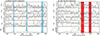 |
Fig. 1. Polarisation spectra of SN 2021irp before and after the ISP subtraction. (a) Total polarisation P, Stokes parameters Q and U, polarisation angle θ, and S/N before the ISP subtraction at a phase of 203.0 d (black lines). The data are binned to 50 Å per point. The grey lines in the background of each plot are the unbinned total-flux spectra at the same epoch. The ISP is described by PISP = 0.32 %, θISP = 8.8°(red lines). The blue hatching shows the adopted wavelength range for the ISP-dominated components. (b) Same as (a), but after the ISP subtraction. The brown and blue lines show the transmission curves of the R band and FILT_815_13. The red hatching shows the adopted wavelength range for the estimate of the continuum polarisation. |
Based on the polarisation degree, the ISP can, in principle, originate from dust either in the Milky Way (MW) or in the host, according to the above empirical relation. However, it might be reasonable to consider the origin as MW dust because the extinction in the MW is higher than that in the host by an order of magnitude. The polarisation angle may support this interpretation, although it is not definitive. Based on the 3D dust map (Green et al. 2019), the majority of the dust responsible for the MW extinction is located around 380–400 pc away from us. The polarisation angles of field stars at similar locations are relatively similar to the observed angle for the ISP (∼0°; Mathewson & Ford 1970). In any case, this speculation on the origin of the ISP does not affect our results, which are described below.
3.2. Intrinsic supernova polarisation
Figure 1b shows the polarisation spectrum after the ISP subtraction. It shows relatively constant polarisation angles over the observed wavelength region with high polarisation degrees (∼0.8%) at wavelength regions without strong lines and low degrees at strong emission lines and at bluer wavelengths where there are many weak blended lines. These polarisation properties can be interpreted as a high continuum polarisation whose degrees and angles are constant through wavelengths and depolarised at wavelengths of emission lines by the multiple scattering and/or absorption.
For the estimation of the continuum polarisation, we averaged the signals of the polarisation spectrum in the wavelength regions from 6800 Å to 7200 Å and from 7820 Å to 8140 Å (see the red hatching in Figure 1b; e.g. Chornock et al. 2010; Nagao et al. 2019, 2021, 2024a), after the ISP subtraction. The derived continuum polarisation at 203.0 d is as follows: P = 0.77 ± 0.06, θ = 100.5° ± 2.5°. The values from imaging polarimetry at different epochs are consistent with those from spectro-polarimetry, all showing a ∼1% level of polarisation with an angle of ∼100°. The R-band polarisation at 190.1 d is P = 0.88 ± 0.58, θ = 110.2° ± 18.8°, while the polarisation through the FILT_815_13 filter at 261.8 d is P = 1.47 ± 0.40, θ = 116.8° ± 8.7°.
The high continuum polarisation in SN 2021irp, which is mainly powered by CSM interaction (see Paper I), implies an aspherical electron-scattering-dominated photosphere and, thus, an aspherical CSM interaction. This high polarisation degree (∼0.8%) corresponds to a photosphere of an oblate ellipsoid with axis ratios of 0.8, 0.7, 0.5 and 0.2 towards viewing angles θobs of ∼90°, ∼60°, ∼40°, and ∼30° from the polar direction, respectively, based on the electron-scattering atmosphere model by Hoflich (1991). This suggests that the CSM structure should be aspherical, for instance, with a disc, jet, or clumpy geometry. The constant polarisation angles from ∼190 to ∼260 d imply that the aspherical structure of the scattering regions remains constant at least during this period. As an approximation, we assume that the asphericity of the photosphere in an SN interacting with disc-like CSM with a half-opening angle of θ0 is similar to that of an oblate ellipsoid with axis ratio of tan(θ0)/2, although the actual shape of the photosphere is more complicated (see Section 5). To get a high polarisation degree of ≳0.8%, the values of θ0 should be ≲58°, ≲55°, ≲45° and ≲22° for θobs of ∼90°, ∼60°, ∼40°, and ∼30°, respectively (Hoflich 1991, see also Uno et al. 2023b, for more details). Additionally, since the viewing angle of SN 2021irp should be a CSM-free direction (see Paper I), the viewing angle should satisfy the following condition: θobs ≲ 90° − θ0. Taking these conditions into account, we can rule out very large opening angles for the disc, and roughly conclude that θ0 ≲ 50°. A more detailed discussion on the CSM geometry can be found in Section 5.
In Fig. 2, we show the evolution of the continuum polarisation in SN 2021irp compared to other Type IIn SNe, as collated in Bilinski et al. (2024). The sample of SNe with detected polarisation at such late phases is small. The polarisation observed in SN 2021irp is similar to that observed in SN 2010jl and SN 2017hcc, assuming linear evolution of the polarisation between the observations at ∼50 d and ∼350 d for SN 2017hcc. We do not have observations of SN 2021irp at early times, but we note that SN 2017hcc was observed to have an extremely large ∼6% polarisation at pre-peak (Mauerhan et al. 2024).
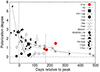 |
Fig. 2. Time evolution of the continuum polarisation in SN 2021irp, compared to those of Type IIn SNe in Bilinski et al. (2024). Here, the peak date for SN 2021irp is set to the date of the maximum magnitude in the ATLAS-o-band light curve as 59331.3 (MJD), although the actual peak was not caught by the observations. |
4. Light curve modelling
We calculated the bolometric luminosity from the interaction shock between the SN ejecta and a disc-shaped CSM (Ldisc) using the light curve model presented in Uno et al. (2023b), which is a modified version of the models by Moriya et al. (2013), Nagao et al. (2020). We note that the explosion date for SN 2021irp is well constrained by observations, with an uncertainty of ∼3 d, despite the fact that the majority of the first ∼100 days of the SN were not observed (see Paper I for details).
4.1. Supernova ejecta properties
For simplicity, we assumed typical ejecta properties for a Type II SN as follows: an ejecta mass of Mej = 10 M⊙ and kinetic energy of the ejecta of Eej = 1051 erg.
For the density profile of the ejecta, we adopted the double power-law distribution (e.g. Moriya et al. 2013), which is derived from hydrodynamics simulations (e.g. Matzner & McKee 1999) and expressed as
![Mathematical equation: $$ \begin{aligned} \widetilde{\rho }_{\mathrm{ej}} (v_{\mathrm{ej}},t) = \left\{ \begin{array}{l} \frac{1}{4 \pi (n-\delta )} \frac{[2(5-\delta )(n-5) E_{\mathrm{ej}}]^{\frac{n-3}{2}}}{[(3-\delta )(n-3) M_{\mathrm{ej}}]^{\frac{n-5}{2}}} t^{-3} v_{\mathrm{ej}}^{-n} \;\;\;\; (v_{\mathrm{ej}} > v_{t})\\ \frac{1}{4 \pi (n-\delta )} \frac{[2(5-\delta )(n-5) E_{\mathrm{ej}}]^{\frac{\delta -3}{2}}}{[(3-\delta )(n-3) M_{\mathrm{ej}}]^{\frac{\delta -5}{2}}} t^{-3} v_{\mathrm{ej}}^{-\delta } \;\;\;\; (v_{\mathrm{ej}} < v_{t}) \end{array} ,\right. \end{aligned} $$](/articles/aa/full_html/2025/10/aa53793-25/aa53793-25-eq1.gif) (1)
(1)
where vej(r, t) (= r/t) is the SN ejecta velocity at radius, r, and time, t, and
![Mathematical equation: $$ \begin{aligned} v_{t} = \left[ \frac{2(5-\delta )(n-5)E_{\mathrm{ej}}}{(3-\delta )(n-3)M_{\mathrm{ej}}} \right]^{\frac{1}{2}}. \end{aligned} $$](/articles/aa/full_html/2025/10/aa53793-25/aa53793-25-eq2.gif) (2)
(2)
Hereafter, we use ρej(r, t), which has the independent variable r instead of vej and is given by  . Here, we assume that n = 12 and δ = 1, which are typical values for Type II SNe (e.g. Matzner & McKee 1999).
4.2. CSM properties
As an initial distribution of the CSM, we adopted a disc structure with a half-opening angle, θ0. We expressed the radial distribution of the CSM as
 (3)
(3)
The isotropic mass-loss rate ( ) is linked with the actual mass-loss rate (Ṁdisc) for the disc-shaped CSM as follows:
  . Here, Ωdisc is the solid angle of the CSM disc, and ωdisc = Ωdisc/4π = sin θ0. The actual mass-loss rate (Ṁdisc) expresses the total mass that is ejected per unit time. Thus, for the same value of Ṁdisc, the density of the CSM, which controls the evolution of the CSM interaction, depends on the half-opening angle of the disc. On the contrary, the isotropic mass-loss rate (
 ) is a good indicator to help us understand the density of the CSM and thus the evolution of the interaction shock. This distribution with r−2 is expected for a steady mass loss from a progenitor system with a constant mass-loss rate of Ṁdisc and wind velocity of vcsm. The CSM velocity is set to vcsm = 50 km s−1, which is consistent with the value estimated for SN 2021irp from the high-dispersion spectroscopic observation (≲85 km s−1; see Paper I). The location of the inner edge of the disc is assumed to correspond to the progenitor radius before the explosion: Rcsm = Rp. In the outer region, the CSM is assumed to extend to infinity.
4.3. CSM interaction
We calculated the evolution of the shocked shell from the equation of motion of the shock, assuming the shell is physically thin compared to its radius (see Uno et al. 2023b, for details). This is expressed as
![Mathematical equation: $$ \begin{aligned} M_{\mathrm{sh}} (t) \frac{dv_{\mathrm{sh}}(t)}{dt}&= 4 \pi r_{\mathrm{sh}}^{2}(t) \Bigl [ \rho _{\mathrm{ej}} (r_{\mathrm{sh}}(t),t) \left( v_{\mathrm{ej}}(r_{\mathrm{sh}}(t),t)-v_{\mathrm{sh}}(t) \right)^{2} \nonumber \\&\quad - \rho _{\mathrm{csm}} (r_{\mathrm{sh}}(t)) \left( v_{\mathrm{sh}}(t)-v_{\mathrm{csm}} \right)^{2} \Bigr ], \end{aligned} $$](/articles/aa/full_html/2025/10/aa53793-25/aa53793-25-eq8.gif) (4)
(4)
where vsh(t) is the velocity of the shocked shell at a given time, t, and Msh(t) is the total mass of the shocked SN ejecta and CSM,
 (5)
(5)
Here rej, max(t) = vej, maxt, and vej, max is the original velocity of the outermost layer of the SN ejecta before the interaction. Here, we assume rej, max(t)≫rsh(t) at any time. By numerically solving Eq. (4), we obtain the values of rsh(t) and vsh(t).
4.4. Bolometric luminosity
We calculated the bolometric luminosity from the interaction between the assumed SN ejecta and CSM, following the same procedures described in Uno et al. (2023b). First, we considered the luminosity from the interaction with a spherically symmetric CSM. A fraction of the released energy by the interaction is converted into radiation (see, e.g. Moriya et al. 2013; Nagao et al. 2020), as follows:
 (6)
(6)
where ε is the conversion efficiency from kinetic energy to radiation, and
 (7)
(7)
We considered the optical-depth effects within the shock shell towards this generated radiation, as in Uno et al. (2023b). We calculated a light curve from the interaction as a superposition of gas shells with photons that are generated at each time (see Nagao et al. 2020). Thus, the light curve from the interaction with the spherical CSM is computed as follows:
 (8)
(8)
where
 (9)
(9)
and
 (10)
(10)
 (11)
(11)
where ΔRsh(t) is the thickness of the shock shell, and κes is the mass scattering coefficient for the electron scattering. Throughout this study, we adopted the value of  as the opacity in the fully ionised gas mainly composed of hydrogen and helium with the solar abundance.
In the case of the interaction with the disc CSM, the CSM is confined into the disc region and the density scale of the CSM disc coincides with the value in the case of the spherical CSM with  . Therefore, we calculated the bolometric light curves to find the bolometric luminosity from the interaction between the SN ejecta and the disc CSM as:
 (12)
(12)
4.5. Comparison of the light curve models with observations
We derived the best-fit light curve (LC) models for the bolometric light curve of SN 2021irp, which was approximated via blackbody fitting using the optical photometry (see Paper I), with the mass-loss rate (Ṁdisc), the opening angle (θ), and conversion efficiency (ϵ) as free parameters. We investigated the ranges of these parameters, namely:  M⊙ yr−1, 15 ≦ θ ≦ 90 degrees and 0.1 ≦ ϵ ≦ 1.0.
To check whether a significant bolometric correction is required for our estimate of the bolometric luminosity of SN 2021irp, we compared the luminosity in the optical region, measured from a spectrum obtained at 203 d, to the luminosity of the blackbody fit to the optical photometry at the same epoch, in the same wavelength region. The difference in luminosities is only ∼6%, implying no bolometric correction is required. We lack the data to make this comparison in the UV or IR.
Figure 3 shows the residuals between the observations and the best-fit models for all combinations of Ṁdisc and θ and the energy conversion efficiency for each best-fit model. Here, the residuals are defined as in Uno et al. (2023b): Σ[(model − data)/data]2. we note that we did not use the late-phase data (> 200 d after the explosion) in the light curve fitting, so as to avoid the part with the accelerated decay (see Paper I for the discussions on possible origins of this decay). The total number of the data points of the bolometric light curve that we used for the fitting (< 200 d after the explosion) is 94. Thus, the residual per data point was derived by dividing the above residual by 94. According to the obtained residuals, the realistic values for the mass-loss rate and the half-opening angle (from the models with residuals ≲1.0) are in the ranges of  M⊙ yr−1 and 30 ≲ θ0 ≲ 90 degrees, respectively. In a dense CSM interaction, the conversion from the kinetic to thermal energy becomes effective, where the conversion efficiency is close to unity (e.g. Maeda & Moriya 2022). The best-fit models show high values of the conversion efficiency from ∼0.5 to 1.0 (Figure 3).
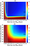 |
Fig. 3. Results for the light curve fitting. (a): Residual between the observed bolometric light curve and the best-fit model for each combination of the mass-loss rate (Ṁdisc) and the half-opening angle (θ0). (b): Energy conversion efficiency (ϵ) for each best-fit model. |
5. Derived circumstellar material properties
Figure 4 shows the light curves for several sets of best-fit parameters with relatively small residuals, and Fig. 5 shows the time evolution of the mass and location of the shock shell for each parameter set. The assumed density distribution of the CSM (ρ ∝ r−2) can roughly explain the decline rate at early phases (< 200 d). The steep decline of the optical luminosity after approximately 250 d is most likely caused by dust formation (see Paper I), but even after including the IR luminosity arising from the dust, the light curve deviates from the best-fit models at late phases. This might imply that the actual CSM density distributions are slightly steeper than the assumed one (s = 2). The total CSM mass swept up by the interaction shock is at the level of at least several solar masses already ∼200 d after the explosion. If the assumed SN parameters are correct, the minimum value for the necessary CSM mass would be ∼2 M⊙ for the best-fit case with  M⊙ yr−1. This necessary CSM mass is within the range of the diversity in Type IIn SNe (e.g. Smith 2017).
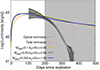 |
Fig. 4. Time evolution of the luminosity for several well-fitting models. The bolometric luminosity estimated with the optical photometry is shown with black open circles, while the total luminosity from the optical and infrared photometry is with red open circles. Model parameters are listed in the figure. We excluded the late-phase data (t ≳ 200 d; gray hatching) from the light curve fitting. |
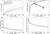 |
Fig. 5. Time evolution of the shock shell mass (top left), shock radius (top right), shock velocity (bottom left) and optical depth of the shock shell (bottom right) for several well-fitting models. The adopted model parameters are the same in Fig. 4. We excluded the late-phase data (t ≳ 200 d; grey hatching) from the light curve fitting. The black open circles in the top right panel are the blackbody radii of the optical component from the two blackbody fitting in Paper I. |
The expected shock radii in the best-fit cases are always larger than the observed black-body radius (Figure 5). This suggests that the CSM interaction is aspherical and the photosphere should be localised around the interaction regions. The expected shock radius is several ×1015 cm at ∼200 d after the explosion. Assuming a wind velocity of ∼50 km s−1, this distance corresponds to an expansion time of ∼10 years, implying that the progenitor ejected ≳2 M⊙ within the last ∼10 years before the explosion. In addition, the shock velocities in the best-fit cases (∼3000 km s−1 at a few hundred days after the explosion) are much lower than the observed velocities in the Balmer lines (∼8000 km s−1; see Paper I). This suggests that the emitting regions for the broadest part of the Balmer lines and possibly the photospheric radiation should be in the H-rich SN ejecta rather than in the shock shell. In particular, we are looking at parts of the H-rich SN ejecta heated by the aspherical CSM interaction. In fact, the optical depth of the shock shell from the best-fit models is much higher than unity at the phase of ∼200 d, when we already observe broad Balmer lines in the spectra of SN 2021irp (Figure 5). This is also true for the spherical models with θ0 = 90°. Therefore, the CSM interaction is required to be aspherical so that we can see the SN ejecta where the broad Balmer lines arise at this phase of the SN when the shocked shell is optically thick.
Our light curve models demonstrate that the bolometric light curve can be explained by a normal Type II SN (an explosion of a red supergiant with an ejecta mass of ∼10 M⊙ and explosion energy of ∼1051 erg) interacting with several solar masses of CSM in a disc shape. We can also consider other aspherical morphologies for the CSM: a jet-like morphology where the CSM has a continuous radial distribution extending from a spherical cap with a small opening angle; or a blob-like morphology, which is similar but is not continuously distributed. The light curves in the cases of jet-like or blob-like CSM, would be equivalent to the disc models with a small half-opening angle of the disc, which are not preferred by the light curve fitting (see Figure 3). In order to obtain similar luminosities with the jet or blob CSM distribution, we need a denser CSM than in the disc CSM case. For example, the density scale for the interaction with jet-like CSM with a half-opening angle of ∼30° corresponds to the disc case with ∼8°. In addition, the shapes of the broad Balmer lines are rather symmetric towards the red and blue sides before the acceleration of the light curve decline (≲250 d after the explosion; see Paper I), which corresponds to the likely onset of dust formation. This disfavours the scenarios with jet- or blob-like CSM, where clear multiple peaks (for bipolar jet-like CSM) or a shifted peak to the red or blue side (for a blob-like CSM) would be expected in the observed Balmer lines.
Combining the above considerations with the observed persistent high continuum polarisation in SN 2021irp (see Section 3), we conclude that the radiation should mainly come from an aspherical (i.e., toroidal) photosphere and that this photosphere is located around the ring-shaped CSM interaction region, as shown in Figure 6.
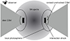 |
Fig. 6. Schematic picture of the aspherical CSM interaction in SN 2021irp. |
6. Discussion
6.1. Origin of the broad Balmer lines
SN 2021irp notably shows strong broad (FWHM ∼ 8000 km s−1 Balmer lines at least from 200 d after the explosion, rather than the narrow or intermediate width lines which are observed in Type IIn SNe and regarded as a sign of strong interaction with H-rich CSM. This cannot be explained with the classical picture of Type IIn SNe with a spherical CSM interaction (e.g. Figure 1 in Smith 2017) and therefore provides an opportunity to improve our understanding of the radiation processes in an aspherical CSM interaction. In fact, the observed BB radius of SN 2021irp supports the possibility of such an aspherical CSM interaction (see Paper I).
Smith et al. (2015) proposed a qualitative picture for the photometric and spectroscopic behaviour of interacting Type II SNe with a disc CSM in order to explain the observations of PTF11iqb (see also Smith 2017, and references therein). At early phases, the CSM interaction region, which lies in the equatorial plane, is hidden by the opaque SN ejecta in the polar directions. Therefore, in this phase, the system would resemble a luminous Type II SN, where its spectrum will be similar to those of normal Type II SNe with broad lines but without narrow lines. Since the photosphere in the SN ejecta in the polar directions recedes inward with time, we eventually see the interaction region. At this point, we would observe it as an interacting SN with a spectrum with intermediate width lines arising from the post-shock CSM. Nagao et al. (2020) quantitatively investigated this picture for Type II SNe interacting with a CSM disc by calculating the shock evolution and radiative transfer. Their study demonstrated that such a phase of hidden CSM interaction can last only for the first several tens of days. Therefore, the location of the CSM interaction should already be exposed outside of the photosphere in the SN ejecta in the polar directions at the epochs of our spectroscopic observations (Phases ≳200 d after the explosion), and we can naively expect to see narrow Balmer lines. However, SN 2021irp does not fit this picture, as it shows strong broad Balmer lines and it does not show strong narrow lines in its spectra (see Paper I).
We propose a modified picture for the photometric and spectroscopic behaviour of interacting Type II SNe with disc CSM, as shown in Figure 6. After the interaction runs over the photosphere in the SN ejecta in the polar directions, the high-energy photons from the interaction shocks heat and re-ionise the already recombined hydrogen gas, creating an optically thick region locally around the interaction. This reprocesses the original radiation created in the interaction region into radiation from the local ‘photosphere’ located in the SN ejecta around the interaction region (continuum plus broad lines). The observed blackbody temperature should be ∼6000 K, consistent with the recombination temperature of hydrogen, similar to the temperature observed in Type II SNe during the plateau phase (6000–8000 K, see e.g. Faran et al. 2018). This is indeed what we observe for SN 2021irp (see Paper I).
Since the local photosphere at this phase is located in a relatively outer region in the SN ejecta and distorted into the CSM disc direction, the line-forming regions are placed in higher velocity parts of the SN ejecta and, thus, higher-velocity-parts-enhanced and emission-dominated Balmer lines are expected even at late phases. Notably, in this case, the photosphere is not spherical but it should have a torus-like shape. This might explain the peculiar shapes of Balmer lines in SN 2021irp, which deviate from a Gaussian (see Paper I).
Comparing SN 2021irp with the Type Ia-CSM SN 2020uem can help support this interpretation. SN 2020uem is a Type Ia SN that has been interpreted as interacting with a similar CSM disc – just as we are suggesting for SN 2021irp, based on its photometric and polarimetric properties (see Uno et al. 2023a,b). As shown in Fig. 7, their bolometric light curves are relatively similar during the phases of SN 2021irp that are not strongly affected by increased extinction from newly formed dust. SN 2020uem also shows a high degree of polarisation (around 1%), which is similar to SN 2021irp. In Fig. 8, we show selected spectra of SN 2021irp and SN 2020uem at similar phases. There are a number of similar features in the spectra, particularly the Ca II NIR triplet and Fe II pseudo-continua. However, SN 2020uem lacks the broad (∼8000 km s−1) emission line features of the Balmer series and He I, instead showing narrow Balmer emission lines (1500 km s−1) with Lorentzian profiles at all times (Uno et al. 2023a).
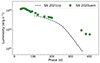 |
Fig. 7. Bolometric light curves of SN 2021irp and SN 2020uem. The luminosity is measured in the B/g-I/i bands for both SNe. |
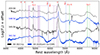 |
Fig. 8. Spectra of SN 2021irp and SN 2020uem, compared at similar epochs. The labels give the phases the spectra were observed at. All spectra are corrected for extinction. |
Our interpretation of the origin of the broad Balmer lines in SN 2021irp naturally explains the different shapes of Balmer lines in the SNe 2021irp and 2020uem, both of which have similar configurations for the main energy source (i.e. interaction with several solar masses of CSM configured in a disc). In the case of SN 2021irp, the SN ejecta is expected to be hydrogen-rich and massive (∼10 M⊙), while SN 2020uem has Type Ia SN ejecta, which is hydrogen-poor and less massive. In the case of SN 2020uem, the SN ejecta around the shock regions cannot produce an optically thick photosphere hiding the interaction regions and the ionised un-shocked CSM due to the lower opacity in a Type Ia SN ejecta. Thus, we see the strong, narrow Balmer lines from the ionised unshocked CSM, unlike the case of SN 2021irp.
6.2. Relations with other types of SNe
Some interacting SNe, known as Type IIn SNe, show strong narrow Balmer lines. These SNe may be explained with spherical CSM interaction as in the classical picture (e.g. Smith 2017). However, if we had observed the system of SN 2021irp from the equatorial plane of the CSM disc, we would also see strong narrow Balmer lines as in Type IIn SNe. For example, SNe 2010jl, 2021acya, and 2021adxl, which all show strong multiple-width components of Balmer lines, might be such cases (Fransson et al. 2014; Brennan et al. 2024; Salmaso et al. 2025). From the light curve modelling of SN 2021irp, we find that the half-opening angle of the CSM disc is between ∼30 − 90°, while the high polarisation rules out very large opening angles (≳50°). If we observe the system of SN 2021irp with random viewing angles based on the assumption of a half-opening angle of 45 degrees, we would observe a 21irp-like SN (dominated by broad Balmer lines) for 30% of all the viewing angles and a Type IIn SNe for the remaining 70%. Since we do not know the rate of 21irp-like SNe, it is not possible to estimate what fraction of Type IIn SNe could originate from similar objects as SN 2021irp observed with edge-on views of the CSM disc. Polarimetry is the key to unveiling SNe interacting with aspherical CSM that are viewed at a viewing angle that causes them to otherwise appear similar to Type IIn that are dominated by spherical CSM interaction. Both types of transients would show narrow Balmer lines and thus should be classified as Type IIn SNe. However, for the former case, we expect to have an aspherical photosphere and thus high polarisation, while we would get low polarisation for the latter case. Understanding the relative rates of each CSM configuration would reveal much about the origins (the progenitors and mass-loss mechanism) of Type IIn SNe, supporting further investigation.
We speculate that broad emission-dominated lines during the photospheric phases in other types of SNe (e.g. some Type IIL SNe, some Type II superluminous SNe, and some Type II SNe as SN 2021irp) might share similar radiation processes. Indeed, the Type IIn SN 2017hcc shows very similar photometric, spectroscopic and polarimetric properties (see Paper I). One possibility is that it is a similar system as SN 2021irp but with a different viewing angle. There might be more 21irp-like objects, observed with different viewing angles, within the population of Type IIn SNe and/or Type II superluminous SNe. Again, the key observation to identify 21irp-like SNe from the zoo of interacting SNe would be polarimetry, which directly traces the shape of the photosphere. In addition, the line profiles, width, and in particular their deviations from a Gaussian shape are useful for recognising these hidden-interaction-powered SNe.
6.3. The progenitor of SN 2021irp
In this subsection, we discuss possible progenitors of SN 2021irp based on the estimated properties of its CSM. The light curve modelling of SN 2021irp indicates that this SN can be explained by a normal Type II SN (i.e. an explosion of an ∼10 M⊙ red supergiant with an explosion energy of ∼1051 erg) interacting with disc CSM of ≳2 M⊙, created within a few decades before the explosion (assuming a wind velocity of ∼50 km s−1). The polarimetric and spectroscopic properties of SN 2021irp also support this interpretation. An interesting point here is that this peculiar SN with a very long duration does not require any peculiar progenitor star. It merely needs a normal massive star similar to those identified as progenitors of Type IIP SNe (e.g. Smartt et al. 2009) but with an extremely large mass ejection just before the explosion. There is some observational evidence that supports this result: the progenitors of Type IIP and Type IIn SNe arise from similar environments (Anderson et al. 2012), and the locations of Type IIn SNe within their host galaxies do not follow the locations of the most intense star formation, as would be expected if they were all to arise from very massive stars (Habergham et al. 2014; Ransome et al. 2022). As for the origin of such massive CSM, any known mass-loss mechanisms in massive stars struggle to eject their outer parts in such a short period just before the explosion (e.g. Smith 2014), although some qualitative ideas for extensive mass ejections at the final evolutionary phases of massive stars have been proposed (e.g. Humphreys & Davidson 1994; Langer et al. 1999; Yoon & Cantiello 2010; Arnett & Meakin 2011; Chevalier 2012; Quataert & Shiode 2012; Soker & Kashi 2013; Shiode & Quataert 2014; Smith & Arnett 2014; Woosley & Heger 2015; Quataert et al. 2016; Fuller 2017).
The observed properties of SN 2021irp, particularly the relatively symmetric shape of the Hα emission line and the smooth light curve evolution, indicate that the CSM distribution is not clumpy or jet-like but a disc-like structure. This might suggest that the mass ejection process is related to binary interaction. Even with known types of mass ejections due to binary interaction, it is difficult to reproduce an mass ejection as extreme as the one we have inferred for SN 2021irp (e.g. Ouchi & Maeda 2017). One possibility is an extreme binary interaction; for instance a common envelope evolution triggered by some unknown mechanism, closely followed by a SN (see Pastorello et al. 2019, for a possible example). Binary interaction is relatively common during the lifetime of progenitor systems of Type II SNe (see e.g. Zapartas et al. 2019) and the majority of massive stars are in multiple systems (see e.g. Moe & Di Stefano 2017; Merle 2024; Sana et al. 2012). However, since the timing of the mass ejection should be within a few decades of the explosion, the unknown mechanism that triggers such an extreme mass ejection should be related to the last burning phases (carbon and/or neon burning) in the progenitor star. For example, expansion of the stellar envelope related to the final burning phases could trigger binary interaction and thus enhance mass ejection during the last decades before the explosion (Murata & Maeda, in prep.).
A suitable progenitor binary system for SN 2021irp should have a separation close enough to trigger this very late stage interaction, but far apart enough so that there would be no extensive history of mass transfer. A closer binary with extensive mass transfer would lead to a hydrogen-poor SN, while a more distant one with no mass transfer would not create the CSM we have observed; instead, it would lead to a Type IIP SN. As SNe with such extensive CSM interaction are rare (Type IIn SNe make up 5–10% of core-collapse SNe, see e.g. Li et al. 2011; Smith et al. 2011; Cold & Hjorth 2023) and these progenitor systems would only be a subset of these SNe, we find that such a fine-tuned (and therefore rare) system is plausible. It is important to increase the sample of these kinds of SNe, and study the diversity among the parameters of the SN ejecta and CSM to shed more light on their origin.
7. Conclusions
The polarimetric observations and light curve modelling presented in this work, supported by the observations and analysis presented in Paper I, show that the bright, long-lived Type II SN 2021irp can be explained as a typical Type II SN interacting with a CSM disc. The estimated mass and half-opening angle of the CSM disc are ≳2 M⊙ (with corresponding mass-loss rate of ∼0.035 − 0.1 M⊙ yr−1) and ∼30 − 50°, respectively. We suggest that this CSM disc was created by some binary interaction process, and that SN 2021irp arises from a usual massive star (with a ZAMS mass of ∼8 − 18 M⊙). The separation and/or a mass ratio of the binary system should be within a specific range of values, which would then lead to an extreme mass ejection in the final decades before the SN, but without stripping the star’s H envelope at an earlier stage.
Studying SNe such as SN 2021irp is important for understanding not only their origin but also the origin of other interacting SNe, which may also be undergoing asymmetric interaction with a CSM disc. We anticipate that there must be some Type IIn SNe that undergo a similar CSM-disc interaction as SN 2021irp, but with a different viewing angle (i.e. the edge-on view). Such Type IIn SNe should have similar photometric evolution but different spectral features, in particular, strong narrow Balmer lines. We emphasise that polarimetry is important to distinguish narrow-line-dominated 21irp-like objects, powered by aspherical CSM interaction with edge-on views of the CSM disc, and Type IIn SNe that are powered by a spherical CSM interaction.
Based on the observational properties of SN 2021irp (and similar SNe), we also propose a new scenario to explain the spectroscopic properties of Type II SNe interacting with a massive disc CSM. At early phases, they show a blue continuum and narrow Balmer lines. Once the interaction regions are hidden by the optically thick SN ejecta, the radiation from the interaction shock and the unshocked CSM is reprocessed, and go on to exhibit a continuum and broad Balmer lines. When the SN ejecta become optically thin, they might start to show a minimal continuum and forbidden lines (so-called nebular spectrum) if the SN ejecta are still bright enough.
Data availability
The final spectropolarimetric data are available at the CDS via anonymous ftp to https://cdsarc.cds.unistra.fr/viz-bin/cat/J/A+A/702/A213
Acknowledgments
T.M.R. is part of the Cosmic Dawn Center (DAWN), which is funded by the Danish National Research Foundation under grant DNRF140. T.M.R. and S. Mattila acknowledge support from the Research Council of Finland project 350458. TN thanks Masaomi Tanaka and Akihiro Suzuki for fruitful discussion. TN and HK acknowledge support from the Research Council of Finland projects 324504, 328898, and 353019. TK acknowledges support from the Research Council of Finland project 360274. C.P.G. acknowledges financial support from the Secretary of Universities and Research (Government of Catalonia) and by the Horizon 2020 Research and Innovation Programme of the European Union under the Marie Skłodowska-Curie and the Beatriu de Pinós 2021 BP 00168 programme, the support from the Spanish Ministerio de Ciencia e Innovación (MCIN) and the Agencia Estatal de Investigación (AEI) 10.13039/501100011033 under the PID2023-151307NB-I00 SNNEXT project, from Centro Superior de Investigaciones Científicas (CSIC) under the PIE project 20215AT016 and the program Unidad de Excelencia María de Maeztu CEX2020-001058-M, and from the Departament de Recerca i Universitats de la Generalitat de Catalunya through the 2021-SGR-01270 grant. K.M. acknowledges support from the Japan Society for the Promotion of Science (JSPS) KAKENHI grant JP24KK0070 and 24H01810. The work is partly supported by the JSPS Open Partnership Bilateral Joint Research Projects between Japan and Finland (K.M. and H.K.; JPJSBP120229923). M.F. is supported by a Royal Society - Science Foundation Ireland University Research Fellowship. N.E.R. acknowledges support from the PRIN-INAF 2022, ‘Shedding light on the nature of gap transients: from the observations to the models. This research was partly based on observations made with the Nordic Optical Telescope (program ID P64-507 & P64-023), owned in collaboration by the University of Turku and Aarhus University, and operated jointly by Aarhus University, the University of Turku and the University of Oslo, representing Denmark, Finland and Norway, the University of Iceland and Stockholm University at the Observatorio del Roque de los Muchachos, La Palma, Spain, of the Instituto de Astrofisica de Canarias. The data presented here were obtained in part with ALFOSC, which is provided by the Instituto de Astrofisica de Andalucia (IAA) under a joint agreement with the University of Copenhagen and NOT. This research was partly based on observations collected at the European Southern Observatory under ESO programmes 108.228K.001 and 108.228K.002.
References
- Anderson, J. P., Habergham, S. M., James, P. A., & Hamuy, M. 2012, MNRAS, 424, 1372 [NASA ADS] [CrossRef] [Google Scholar]
- Appenzeller, I., Fricke, K., Fürtig, W., et al. 1998, Messenger, 94, 1 [Google Scholar]
- Arnett, W. D., & Meakin, C. 2011, ApJ, 741, 33 [NASA ADS] [CrossRef] [Google Scholar]
- Barbon, R., Ciatti, F., & Rosino, L. 1979, A&A, 72, 287 [Google Scholar]
- Beasor, E. R., Smith, N., & Jencson, J. E. 2025, ApJ, 979, 117 [Google Scholar]
- Bilinski, C., Smith, N., Williams, G. G., et al. 2018, MNRAS, 475, 1104 [Google Scholar]
- Bilinski, C., Smith, N., Williams, G. G., et al. 2024, MNRAS, 529, 1104 [Google Scholar]
- Boian, I., & Groh, J. H. 2020, MNRAS, 496, 1325 [CrossRef] [Google Scholar]
- Brennan, S. J., Schulze, S., Lunnan, R., et al. 2024, A&A, 690, A259 [NASA ADS] [CrossRef] [EDP Sciences] [Google Scholar]
- Bruch, R. J., Gal-Yam, A., Schulze, S., et al. 2021, ApJ, 912, 46 [NASA ADS] [CrossRef] [Google Scholar]
- Chevalier, R. A. 2012, ApJ, 752, L2 [NASA ADS] [CrossRef] [Google Scholar]
- Chornock, R., Filippenko, A. V., Li, W., & Silverman, J. M. 2010, ApJ, 713, 1363 [Google Scholar]
- Chugai, N. N. 2001, MNRAS, 326, 1448 [NASA ADS] [CrossRef] [Google Scholar]
- Cold, C., & Hjorth, J. 2023, A&A, 670, A48 [NASA ADS] [CrossRef] [EDP Sciences] [Google Scholar]
- Dilday, B., Howell, D. A., Cenko, S. B., et al. 2012, Science, 337, 942 [NASA ADS] [CrossRef] [Google Scholar]
- Faran, T., Nakar, E., & Poznanski, D. 2018, MNRAS, 473, 513 [NASA ADS] [CrossRef] [Google Scholar]
- Förster, F., Moriya, T. J., Maureira, J. C., et al. 2018, Nat. Astron., 2, 808 [CrossRef] [Google Scholar]
- Fransson, C., Ergon, M., Challis, P. J., et al. 2014, ApJ, 797, 118 [Google Scholar]
- Fraser, M. 2020, R. Soc. Open Sci., 7, 200467 [NASA ADS] [CrossRef] [Google Scholar]
- Fuller, J. 2017, MNRAS, 470, 1642 [NASA ADS] [CrossRef] [Google Scholar]
- González-Gaitán, S., Tominaga, N., Molina, J., et al. 2015, MNRAS, 451, 2212 [CrossRef] [Google Scholar]
- Green, G. M., Schlafly, E., Zucker, C., Speagle, J. S., & Finkbeiner, D. 2019, ApJ, 887, 93 [NASA ADS] [CrossRef] [Google Scholar]
- Habergham, S. M., Anderson, J. P., James, P. A., & Lyman, J. D. 2014, MNRAS, 441, 2230 [CrossRef] [Google Scholar]
- Hamuy, M., Phillips, M. M., Suntzeff, N. B., et al. 2003, Nature, 424, 651 [NASA ADS] [CrossRef] [Google Scholar]
- Hoflich, P. 1991, A&A, 246, 481 [NASA ADS] [Google Scholar]
- Humphreys, R. M., & Davidson, K. 1994, PASP, 106, 1025 [NASA ADS] [CrossRef] [Google Scholar]
- Khazov, D., Yaron, O., Gal-Yam, A., et al. 2016, ApJ, 818, 3 [CrossRef] [Google Scholar]
- Kumar, B., Eswaraiah, C., Singh, A., et al. 2019, MNRAS, 488, 3089 [NASA ADS] [CrossRef] [Google Scholar]
- Langer, N., García-Segura, G., & Mac Low, M.-M. 1999, ApJ, 520, L49 [Google Scholar]
- Leonard, D. C., Filippenko, A. V., Barth, A. J., & Matheson, T. 2000, ApJ, 536, 239 [Google Scholar]
- Li, W., Leaman, J., Chornock, R., et al. 2011, MNRAS, 412, 1441 [NASA ADS] [CrossRef] [Google Scholar]
- Maeda, K., & Moriya, T. J. 2022, ApJ, 927, 25 [NASA ADS] [CrossRef] [Google Scholar]
- Maeda, K., Chandra, P., Moriya, T. J., et al. 2023, ApJ, 942, 17 [NASA ADS] [CrossRef] [Google Scholar]
- Mathewson, D. S., & Ford, V. L. 1970, MmRAS, 74, 139 [Google Scholar]
- Matzner, C. D., & McKee, C. F. 1999, ApJ, 510, 379 [Google Scholar]
- Mauerhan, J. C., Smith, N., Williams, G. G., et al. 2024, MNRAS, 527, 6090 [Google Scholar]
- Merle, T. 2024, Bull. Soc. R. Sci., 93, 170 [NASA ADS] [Google Scholar]
- Moe, M., & Di Stefano, R. 2017, ApJS, 230, 15 [Google Scholar]
- Moriya, T. J., Maeda, K., Taddia, F., et al. 2013, MNRAS, 435, 1520 [CrossRef] [Google Scholar]
- Morozova, V., Piro, A. L., & Valenti, S. 2017, ApJ, 838, 28 [NASA ADS] [CrossRef] [Google Scholar]
- Morozova, V., Piro, A. L., & Valenti, S. 2018, ApJ, 858, 15 [Google Scholar]
- Nagao, T., Cikota, A., Patat, F., et al. 2019, MNRAS, 489, L69 [CrossRef] [Google Scholar]
- Nagao, T., Maeda, K., & Ouchi, R. 2020, MNRAS, 497, 5395 [NASA ADS] [CrossRef] [Google Scholar]
- Nagao, T., Patat, F., Taubenberger, S., et al. 2021, MNRAS, 505, 3664 [NASA ADS] [CrossRef] [Google Scholar]
- Nagao, T., Mattila, S., Kotak, R., & Kuncarayakti, H. 2023, A&A, 678, A43 [NASA ADS] [CrossRef] [EDP Sciences] [Google Scholar]
- Nagao, T., Patat, F., Cikota, A., et al. 2024a, A&A, 681, A11 [NASA ADS] [CrossRef] [EDP Sciences] [Google Scholar]
- Nagao, T., Maeda, K., Mattila, S., et al. 2024b, A&A, 687, L17 [NASA ADS] [CrossRef] [EDP Sciences] [Google Scholar]
- Nyholm, A., Sollerman, J., Tartaglia, L., et al. 2020, A&A, 637, A73 [NASA ADS] [CrossRef] [EDP Sciences] [Google Scholar]
- Ouchi, R., & Maeda, K. 2017, ApJ, 840, 90 [NASA ADS] [CrossRef] [Google Scholar]
- Pastorello, A., Mason, E., Taubenberger, S., et al. 2019, A&A, 630, A75 [NASA ADS] [CrossRef] [EDP Sciences] [Google Scholar]
- Patat, F., & Romaniello, M. 2006, PASP, 118, 146 [Google Scholar]
- Patat, F., Taubenberger, S., Benetti, S., Pastorello, A., & Harutyunyan, A. 2011, A&A, 527, L6 [NASA ADS] [CrossRef] [EDP Sciences] [Google Scholar]
- Quataert, E., & Shiode, J. 2012, MNRAS, 423, L92 [NASA ADS] [CrossRef] [Google Scholar]
- Quataert, E., Fernández, R., Kasen, D., Klion, H., & Paxton, B. 2016, MNRAS, 458, 1214 [NASA ADS] [CrossRef] [Google Scholar]
- Ransome, C. L., Habergham-Mawson, S. M., Darnley, M. J., James, P. A., & Percival, S. M. 2022, MNRAS, 513, 3564 [CrossRef] [Google Scholar]
- Reilly, E., Maund, J. R., Baade, D., et al. 2017, MNRAS, 470, 1491 [NASA ADS] [CrossRef] [Google Scholar]
- Reynolds, T. M., Nagao, T., Gottumukkala, R., et al. 2025, A&A, 702, A212 [NASA ADS] [CrossRef] [EDP Sciences] [Google Scholar]
- Salmaso, I., Cappellaro, E., Tartaglia, L., et al. 2025, A&A, 695, A29 [NASA ADS] [CrossRef] [EDP Sciences] [Google Scholar]
- Sana, H., de Mink, S. E., de Koter, A., et al. 2012, Science, 337, 444 [Google Scholar]
- Schlegel, E. M. 1990, MNRAS, 244, 269 [NASA ADS] [Google Scholar]
- Shiode, J. H., & Quataert, E. 2014, ApJ, 780, 96 [Google Scholar]
- Smartt, S. J. 2015, PASA, 32, e016 [NASA ADS] [CrossRef] [Google Scholar]
- Serkowski, K., Mathewson, D. S., & Ford, V. L. 1975, ApJ, 196, 261 [NASA ADS] [CrossRef] [Google Scholar]
- Smartt, S. J., Maund, J. R., Hendry, M. A., et al. 2004, Science, 303, 499 [NASA ADS] [CrossRef] [Google Scholar]
- Smartt, S. J., Eldridge, J. J., Crockett, R. M., & Maund, J. R. 2009, MNRAS, 395, 1409 [CrossRef] [Google Scholar]
- Smith, N. 2014, ARA&A, 52, 487 [NASA ADS] [CrossRef] [Google Scholar]
- Smith, N. 2017, in Handbook of Supernovae, eds. A. W. Alsabti, & P. Murdin, 403 [Google Scholar]
- Smith, N., & Andrews, J. E. 2020, MNRAS, 499, 3544 [NASA ADS] [CrossRef] [Google Scholar]
- Smith, N., & Arnett, W. D. 2014, ApJ, 785, 82 [NASA ADS] [CrossRef] [Google Scholar]
- Smith, N., Chornock, R., Silverman, J. M., Filippenko, A. V., & Foley, R. J. 2010, ApJ, 709, 856 [NASA ADS] [CrossRef] [Google Scholar]
- Smith, N., Li, W., Filippenko, A. V., & Chornock, R. 2011, MNRAS, 412, 1522 [NASA ADS] [CrossRef] [Google Scholar]
- Smith, N., Mauerhan, J. C., Cenko, S. B., et al. 2015, MNRAS, 449, 1876 [Google Scholar]
- Soker, N., & Kashi, A. 2013, ApJ, 764, L6 [Google Scholar]
- Tody, D. 1986, in Instrumentation in astronomy VI, ed. D. L. Crawford, Society of Photo-Optical Instrumentation Engineers (SPIE) Conference Series, 627, 733 [Google Scholar]
- Tody, D. 1993, in Astronomical Data Analysis Software and Systems II, eds. R. J. Hanisch, R. J. V. Brissenden, & J. Barnes, Astronomical Society of the Pacific Conference Series, 52, 173 [Google Scholar]
- Tonry, J. L., Denneau, L., Heinze, A. N., et al. 2018, PASP, 130, 064505 [Google Scholar]
- Uno, K., Maeda, K., Nagao, T., et al. 2023a, ApJ, 944, 203 [NASA ADS] [CrossRef] [Google Scholar]
- Uno, K., Nagao, T., Maeda, K., et al. 2023b, ApJ, 944, 204 [Google Scholar]
- Van Dyk, S. D., Li, W., & Filippenko, A. V. 2003, PASP, 115, 1 [NASA ADS] [CrossRef] [Google Scholar]
- Wang, L., Wheeler, J. C., & Höflich, P. 1997, ApJ, 476, L27 [NASA ADS] [CrossRef] [Google Scholar]
- Woosley, S. E., & Heger, A. 2015, ApJ, 810, 34 [NASA ADS] [CrossRef] [Google Scholar]
- Yaron, O., Perley, D. A., Gal-Yam, A., et al. 2017, Nat. Phys., 13, 510 [NASA ADS] [CrossRef] [Google Scholar]
- Yoon, S.-C., & Cantiello, M. 2010, ApJ, 717, L62 [NASA ADS] [CrossRef] [Google Scholar]
- Zapartas, E., de Mink, S. E., Justham, S., et al. 2019, A&A, 631, A5 [NASA ADS] [CrossRef] [EDP Sciences] [Google Scholar]
The magnitude here is in the orange (o) band of the Asteroid Terrestrial-impact Last Alert System (ATLAS; Tonry et al. 2018; Smith & Andrews 2020), corresponding approximately to r + i.
All Tables
All Figures
|
Fig. 1. Polarisation spectra of SN 2021irp before and after the ISP subtraction. (a) Total polarisation P, Stokes parameters Q and U, polarisation angle θ, and S/N before the ISP subtraction at a phase of 203.0 d (black lines). The data are binned to 50 Å per point. The grey lines in the background of each plot are the unbinned total-flux spectra at the same epoch. The ISP is described by PISP = 0.32 %, θISP = 8.8°(red lines). The blue hatching shows the adopted wavelength range for the ISP-dominated components. (b) Same as (a), but after the ISP subtraction. The brown and blue lines show the transmission curves of the R band and FILT_815_13. The red hatching shows the adopted wavelength range for the estimate of the continuum polarisation. |
| In the text | |
|
Fig. 2. Time evolution of the continuum polarisation in SN 2021irp, compared to those of Type IIn SNe in Bilinski et al. (2024). Here, the peak date for SN 2021irp is set to the date of the maximum magnitude in the ATLAS-o-band light curve as 59331.3 (MJD), although the actual peak was not caught by the observations. |
| In the text | |
|
Fig. 3. Results for the light curve fitting. (a): Residual between the observed bolometric light curve and the best-fit model for each combination of the mass-loss rate (Ṁdisc) and the half-opening angle (θ0). (b): Energy conversion efficiency (ϵ) for each best-fit model. |
| In the text | |
|
Fig. 4. Time evolution of the luminosity for several well-fitting models. The bolometric luminosity estimated with the optical photometry is shown with black open circles, while the total luminosity from the optical and infrared photometry is with red open circles. Model parameters are listed in the figure. We excluded the late-phase data (t ≳ 200 d; gray hatching) from the light curve fitting. |
| In the text | |
|
Fig. 5. Time evolution of the shock shell mass (top left), shock radius (top right), shock velocity (bottom left) and optical depth of the shock shell (bottom right) for several well-fitting models. The adopted model parameters are the same in Fig. 4. We excluded the late-phase data (t ≳ 200 d; grey hatching) from the light curve fitting. The black open circles in the top right panel are the blackbody radii of the optical component from the two blackbody fitting in Paper I. |
| In the text | |
|
Fig. 6. Schematic picture of the aspherical CSM interaction in SN 2021irp. |
| In the text | |
|
Fig. 7. Bolometric light curves of SN 2021irp and SN 2020uem. The luminosity is measured in the B/g-I/i bands for both SNe. |
| In the text | |
|
Fig. 8. Spectra of SN 2021irp and SN 2020uem, compared at similar epochs. The labels give the phases the spectra were observed at. All spectra are corrected for extinction. |
| In the text | |
Current usage metrics show cumulative count of Article Views (full-text article views including HTML views, PDF and ePub downloads, according to the available data) and Abstracts Views on Vision4Press platform.
Data correspond to usage on the plateform after 2015. The current usage metrics is available 48-96 hours after online publication and is updated daily on week days.
Initial download of the metrics may take a while.