| Issue |
A&A
Volume 702, October 2025
|
|
|---|---|---|
| Article Number | A13 | |
| Number of page(s) | 12 | |
| Section | Astrophysical processes | |
| DOI | https://doi.org/10.1051/0004-6361/202554147 | |
| Published online | 26 September 2025 | |
Exploring jet structure and dynamics in short gamma-ray bursts: A case study on GRB 090510
1
Center for Theoretical Physics, Polish Academy of Sciences, Al. Lotników 32/46, 02-668 Warsaw, Poland
2
Division of Science, National Astronomical Observatory of Japan, 2-21-1 Osawa, Mitaka, Tokyo 181-8588, Japan
3
Department of Astronomical Science, The Graduate University for Advanced Studies, SOKENDAI, Shonankokusaimura, Hayama, Miura District, Kanagawa 240-0115, Japan
4
Space Science Institute, 4765 Walnut St Ste B, Boulder, CO 80301, USA
5
Nevada Center for Astrophysics, University of Nevada, 4505 Maryland Parkway, Las Vegas, NV 89154, USA
⋆ Corresponding authors: This email address is being protected from spambots. You need JavaScript enabled to view it.
; This email address is being protected from spambots. You need JavaScript enabled to view it.
; This email address is being protected from spambots. You need JavaScript enabled to view it.
Received:
15
February
2025
Accepted:
16
July
2025
Abstract
Observations of gamma-ray bursts (GRBs) at high energies enable the emission processes of these still puzzling events to be investigated. In this study, we perform general relativistic magnetohydrodynamic simulations to investigate GRB 090510, a peculiar short GRB detected by Fermi-LAT. Our primary goal is to model the energetics, jet structure, variability, and opening angle of the burst to understand its underlying physical conditions. We tested both 2D and 3D models and estimated the variability timescales. The predicted energetics and the jet opening angle reconcile with the observed ones with 1σ when considering that the jet opening angles also evolve with redshift. Furthermore, we extended our analysis by incorporating dynamical ejecta into selected models to study their impact on jet collimation at smaller distances. In addition, we investigated a suite of models exhibiting a broad range of observable GRB properties, thereby extending our understanding beyond this specific event.
Key words: magnetohydrodynamics (MHD) / gamma-ray burst: general / stars: jets / gamma-ray burst: individual: GRB 090510
© The Authors 2025
 Open Access article, published by EDP Sciences, under the terms of the Creative Commons Attribution License (https://creativecommons.org/licenses/by/4.0), which permits unrestricted use, distribution, and reproduction in any medium, provided the original work is properly cited.
This article is published in open access under the Subscribe to Open model. This email address is being protected from spambots. You need JavaScript enabled to view it. to support open access publication.
1. Introduction
Gamma-ray bursts (GRBs) are intense pulses of high-energy radiation emitted by ultra-relativistic jets aligned with our line of sight from Earth (Kumar & Zhang 2015; Levan 2018; Paczynski 1986). The observed bursts fall into two categories based on their T90 duration (Kouveliotou et al. 1993): short GRBs lasting less than 2 seconds are generally attributed to the mergers of compact binaries (Eichler et al. 1989), while long GRBs (T90 < 2 s) are thought to be driven by the collapse of massive stars (MacFadyen & Woosley 1999). In both cases, a fast jet is emitted along the symmetry axis of the central engine. Several mechanisms of powering these relativistic jets have been proposed, including the Blandford–Znajek (BZ) process from a rotating black hole (Blandford & Znajek 1977), magnetized neutrino-driven winds (Dessart et al. 2008; Rosswog et al. 2003), and spin-down of a magnetar (Metzger et al. 2011; Ciolfi 2018).
These relativistic jets are collimated, and the collimation degree is characterized by a half jet opening angle, θj. However, estimating θj poses a significant challenge, as it demands meticulous observations and a multiwavelength analysis, which is often hindered due to the scarcity of observations or the limited availability of observation programs and telescope time. Moreover, these observed limitations impede the study of θj and properties such as jet variability, adding more complexity to our understanding of jet dynamical properties. Various methods of determining θj from observational data exist (Frail et al. 2001; Bloom et al. 2003; Soderberg et al. 2006; Pian et al. 2006; Watson et al. 2006; Ghirlanda et al. 2007; Berger 2014; Fong et al. 2015; Pescalli et al. 2015; Troja et al. 2016; Goldstein et al. 2016; Lloyd-Ronning et al. 2019a, 2020; Fong et al. 2021). However, it is essential to note that reaching a consensus on a precise value from various methods is challenging, due to the model dependence on microphysical parameters and other scaling assumptions.
In this context, we employ a physical model of jet launching from a GRB central engine to enhance our understanding of the dynamical properties of GRB jets, focusing on θj, variability, and energetics. We propose to model the dynamical evolution of the central engine, produced by the two neutron star (NS) mergers, via high-resolution 2D and 3D general relativistic magnetohydrodynamic (GRMHD) simulations, focusing on the estimation of θj, jet variability, energy, and luminosities. Furthermore, we synergize existing methods to infer the θj (Lu et al. 2012; Amati 2014; Fong et al. 2015; Pescalli et al. 2015; Goldstein et al. 2016) and variability analysis (Bhat et al. 2012; MacLachlan et al. 2013; Golkhou et al. 2015) from observations. The final aim of this paper is to compare the observational properties of GRB 090510, either reported in the literature or derived by us, with the parameters obtained from our simulations.
The paper is structured as follows: Sect. 2 discusses the observational properties of GRB 090510, including the calculation of the bolometric luminosity, isotropic energy, minimum variability timescale calculation, and the jet opening angle determination. Sect. 3 presents the parameters used in our numerical simulations and highlights the similarities and differences between the 2D and 3D models. Sect. 4 shows the results from our numerical simulation. In Sect. 5, we discuss our findings. Finally, in Sect. 6, we summarize our work and draw conclusions.
2. GRB 090510
We chose for our comparison the short GRB 090510. This GRB possesses the plateau emission among the GRBs observed by the Fermi-Large Area Telescope (LAT; Atwood et al. 2009) from August 2008 until August 2016 (Dainotti et al. 2021) with observed redshifts given in the Second Fermi-LAT GRB Catalog (2FLGC; Ajello et al. 2019). To select this GRB, we first considered 19 GRBs analyzed in the 2FLGC from July 2008 until May 2016 following the analysis performed in Dainotti et al. (2021), which were identified as the brightest sources based on maximum likelihood analysis, with a test statistic1 of TS > 64. Of these 19 GRBs, we selected the ones that can be fit with a broken power law (BPL) in the 2FLGC and that have reliable fitting parameters for which the error bars do not exceed the values of the best-fit parameters themselves. This reduced the sample to only three GRBs: GRB 090510, 090902B, and 160509A, with the only short GRB being 090510, making it a particularly interesting case for further investigation. GRB 090510 benefits from comprehensive multiwavelength coverage from Fermi-GBM/LAT and Swift-XRT, with well-constrained redshift, bolometric energy estimates, and variability measurements. These characteristics make it particularly well suited as a benchmark case for our GRMHD jet modeling.
The observational properties of GRB 090510 are summarized in Table 1. We simulate jet models in which the central engine parameters are calibrated to reproduce key observables of this GRB, including its energetics, luminosity, and jet opening angle.
Summary of parameters for GRB 090510.
2.1. Luminosity and isotropic energy
Since the luminosity obtained from the theoretical model is bolometric, we computed the observational counterpart by combining the high-energy (gamma-ray) and X-ray luminosities derived from multiwavelength data. The luminosity was computed in the following way for the total energy band:
 (1)
(1)
where DL(z, ΩM, h) is the luminosity distance computed in the flat ΛCDM cosmological model with ΩM = 0.291 and h = 0.70 in units of 100 km s−1 Mpc−1, F is the measured energy flux, and Emin, Emax are the appropriate energy bandpasses for each instrument we use. The K is the K correction for the cosmic expansion (Bloom et al. 2001):
 (2)
(2)
where the energy spectrum Φ(E) is described by the Band function or a simple power law (PL).
The bolometric luminosity is Lbold = LGBM,LAT + LXRT. The optical contribution, being orders of magnitude lower in luminosity, has a negligible impact on the total energy budget and was thus excluded from the estimate. Multiple studies have conducted spectral analysis of GRB 090510. In our analysis, we adopted the fitting parameters from the optimal model from the combined Fermi-Gamma-ray Burst Monitor (GBM; Meegan et al. 2009) and LAT spectral analysis performed by the Fermi-GBM/LAT collaboration (Ackermann et al. 2010). This best-fit model, applicable during the interval 0.5–1 s, which coincides with the peak high-energy counts in the GBM and LAT light curves (LCs), consists of a Band function with a PL component. The afterglow peak luminosity from the Swift-XRT analysis in the energy range 0.3–10 keV is taken from Lien et al. (2016). This gives a bolometric luminosity of Lbol = (3.90 ± 0.55)×1053 erg s−1 for GRB 090510.
To calculate Eiso, we used the relation
 (3)
(3)
We adopted the bolometric fluence, Sbolo = (5.03 ± 0.25)×10−5 erg cm−2, reported by Ackermann et al. (2010) for the 10 KeV to 30 GeV energy range. This gives a bolometric Eiso of the jet to be (9.97 ± 0.51)×1052 erg. Both the luminosities and energies computed and reported here were used in our comparison with the theoretical simulations.
2.2. Minimum variability timescale
The observed GRB LCs exhibit strong temporal variability. The minimum timescale variability (MTS) refers to the shortest duration within which a significant change in the count rate occurs in the observed LC.
The measure of variability has been a longstanding and debated issue in the literature since its inception (Sari & Piran 1997), and although the variability as an intrinsic property of GRB should have a unique measure, often in the literature, values are discrepant. It is challenging to assess which of the methods is the most reliable. Below, we summarize and discuss two of the most used ones: the Bayesian block (BB) and the wavelet analysis, and we check the value of the variability pertinent to GRB 090510.
The BB method detailed in Scargle et al. (2013) divides the LC into various time intervals of different time widths, closely following true underlying variation in the emission. This algorithm is a non-parametric modeling that employs optimal segmentation analysis on sequential data, with sampling that can be arbitrary in the presence of gaps in the data and different exposure times. In the BB algorithm, each block (or bin in our case) is consistent with a probability distribution function (PDF), and the entire dataset is represented by this collection of finite PDFs. The number of blocks and the edges of the blocks are set via the optimization of a “fitness function”; namely, a goodness-of-fit statistic dependent only on the input data and the regularization parameter. The set of blocks presents no gaps, and there is no overlapping between one block and the other, where the first and last block edges are defined by the first and last data points, respectively. The BB method is based on the additivity of the fitness function, and thus the fitness of a given set of blocks is equal to the sum of the fitness of the individual blocks. The total fitness, Ftot for a given dataset is
 (4)
(4)
where f(Bi) if the fit for an individual block and N is the total number of blocks. The MTS is then obtained by identifying the shortest block width produced by the segmentation. For the analysis, the count rate LC of GRB090510 from the NaI detector of Fermi-GBM in the energy range 10–250 KeV was used. The LC was produced from the GRB data provided by the Fermi Science Support Center (FSSC) and processed using Fermitools. The MTS was calculated to be 32 milliseconds using the BB method.
Complementing the BB approach, wavelet analysis provides an alternative and widely adopted method in GRB variability studies that is particularly effective at isolating transient features across multiple frequencies. Unlike Fourier analysis, wavelet analysis employs basis functions that are localized in both time and frequency domains, enabling the precise identification of variability timescales. Using wavelet analysis, MacLachlan et al. (2013) found an MTS of  milliseconds for GRB 090510. We explore how these observational methods compare with results from numerical simulations in later sections of this paper.
2.3. Jet opening angle from observation
As discussed in the introduction, determining θj is challenging and several observational and theoretical methods have been proposed in the literature (Gao et al. 2009; Ackermann et al. 2010; Corsi et al. 2010; Fan & Wei 2011; He et al. 2011; Panaitescu 2011; Nicuesa et al. 2012; Eichler 2014; Fraija et al. 2016; Goldstein et al. 2016). These studies report values that are typically less than 1° but there are significant uncertainties among the measurements, which often differ by an order of magnitude across different models and approaches. This wide range reflects the inherent uncertainties in deriving θj from observational data, which stem from differences in jet structure assumptions, energy distribution models, assumptions about the density of the circumburst medium, and observational biases (Sari et al. 1999; Chevalier & Li 2000).
To simplify the calculation of θj, the luminosity and energy output of GRBs are typically computed under the assumption of isotropic emission. Despite several methods available to estimate θj (Ghirlanda et al. 2004; Lu et al. 2012; Fong et al. 2015; Goldstein et al. 2016), not all GRBs have this parameter available. In this work, we use an indirect derivation of θj based on the method detailed in Pescalli et al. (2015), in which the Epeak − Eγ relation (Ghirlanda et al. 2004) and the Epeak − Eiso relation (Amati et al. 2002, 2009) have been used and are considered reliable standardizable candles.
From Ghirlanda et al. (2004), we have
 (5)
(5)
where  , AG = 267, and kG = 0.706 ± 0.047 are the normalization and the slopes of the Ghirlanda relation, respectively.
From Amati et al. (2002), we have
 (6)
(6)
where AA = 100 and kA = 0.52 ± 0.06 are the normalization and the slope of the Amati relation, respectively.
By equaling these two equations, we obtain
 (7)
(7)
Substituting constants and performing error propagation, we obtain
 (8)
(8)
which can be further approximated as
 (9)
(9)
Thus, for our GRB, since we have the measure of the isotropic energy (Eiso), the angle θj can be calculated and it is θj ≈ 6°2. We note that independent observational methods have reported smaller values of θj for this GRB, highlighting the methodological dispersion discussed above. Our approach provides a consistent estimate based on isotropic energy, but should be calibrated across a broader GRB sample as more high-quality spectral analyses become available.
However, this value of θj needs to be corrected for the evolution of redshift (z). Following Lloyd-Ronning et al. (2019a), we corrected for the highly statistically significant (≈5σ) anticorrelation between θj and z, with a functional form that reads as follows: θj ∼ (1 + z)−0.75 ± 0.2. Using Eq. (9) and from the evaluation of the observational Eiso = (9.97 ± 0.51)×1052 erg (Sect. 2.1), and z = 0.903, we obtained θj.
We notice, that the value of θj needs to be corrected for the evolution with redshift (z). This relation is not a consequence of observational selection bias alone, but rather reflects an intrinsic redshift evolution in jet opening angles derived using the Efron–Petrosian method (Efron & Petrosian 1992), which accounts for such biases. Therefore, this correction is distinct from the redshift dependence already present through the Eiso in Eq. (9). We obtained θj ≈ 10° after applying the redshift evolution correction.
3. Numerical simulations of GRB engines
Our model of the Short GRB (SGRB) engine adopts a scenario of the binary NS (BNS) merger progenitor but starts when the post-merger compact object has already been formed. The typical outcome of such a scenario is the short-lived stage of a hyper-massive NS (Sekiguchi et al. 2011; Hotokezaka et al. 2013a), which immediately collapses into BH. While a BH is not the only plausible central engine, GRB090510 – our target GRB in this work – has previously been studied and argued to be powered by a BH formed after a NS-NS merger (Ruffini et al. 2016).
3.1. Code
We used the GRMHD code HARM (Gammie et al. 2003; Noble et al. 2006; Sapountzis & Janiuk 2019) to perform a suite of numerical simulations of the accretion flow around a Kerr BH. The HARM code employs a finite-volume shock-capturing scheme to solve the hyperbolic system of partial differential equations in their conservative form. It uses the Harten, Lax, van Leer scheme to numerically compute the corresponding flux function.
The code follows the evolution of the gas and magnetic field by solving the continuity, energy-momentum conservation, and induction equations:
 (10)
(10)
 (11)
(11)
 (12)
(12)
where n is the baryon number density in the fluid frame, uμ is the four-velocity of the gas, and bμ is the magnetic four-vector.
The stress-energy tensor consists of matter and electromagnetic parts:  , where
 (13)
(13)
and
 (14)
(14)
Here u is the internal energy, and p is the gas pressure. The closing equation is that of the pressure relation with density, which defines the equation of state (EoS). In the current simulations, we use an adiabatic form, p = (γad − 1)u, with γad = 4/3.
We adopted dimensionless units, with G = c = M = 1, for our simulations. Thus, the length in the code units is given by rg = GM/c2, and the time is given by tg = GM/c3, where M is the BH mass.
The BH mass was fixed in all our models to be 3M⊙. As we have to compare the results with GRB 090510, all main models were run for a duration of ∼50 000tg, effectively covering 0.6 s in real time, which matches the Fermi-GBM estimated TGBM, 90 for GRB 090510. We restricted the simulation duration to the prompt gamma-ray emission phase, as the modeled jet dynamics are not intended to capture the later afterglow evolution.
3.2. Model
The accretion disk was modeled based on the Fishbone & Moncrief (1976), hereafter FM, solution for a steady-state, pressure-supported fluid in a Kerr BH’s potential. The torus solution was parameterized by two values, the radius of its pressure maximum, rmax, and the radius of the inner cusp location, rin, and it was constructed for a given BH spin, a.
The FM torus is embedded in a poloidal magnetic field. The field geometry resembles that of a circular wire field configuration, and the nonvanishing component of magnetic vector potential is given by
 (15)
(15)
Here, E and K are complete elliptic functions, and A0 is the field normalization constant (Sapountzis & Janiuk 2019). The radius of the circular wire was taken to be the rmax of the FM torus. This magnetic field was scaled across the torus using the plasma-beta factor given by the ratio of initial gas pressure to magnetic pressure, β = p/pmag, with pmag = b2/2. The total mass of the torus was calculated using a physical density scaling in the cgs units. To compute this value, we used an arbitrary mass unit, Munit = 1.5 × 10⁻⁵ M⊙, and hence the torus mass is given by  , where the density, ρ, is expressed in code units.
The FM accretion disk in our model accretes matter into the Kerr BH due to magneto-rotational instability. Magnetized tori launch relativistic jets along the rotation axis of the Kerr BH through the BZ mechanism (Blandford & Znajek 1977). We have employed different models with varying parameters, including the plasma β parameter, BH spin, and disk mass (see Table 2 for model parameters). These variations have provided us with a number of unique jet signatures to be compared with the observed properties. As this study did not incorporate a radiative transport mechanism to explicitly connect simulations to spectral and temporal LC characteristics, we have focused on properties such as total energy, θj, variability timescales, and the Γ factor. These are interconnected physical properties that are key to understanding the observed phenomena.
Models used in the simulation of GRB 090510.
3.2.1. Dynamical ejecta
We extended the parameter space to include two models with dynamical ejecta (DE) setups, which depict GRB environments more realistically. This enables the exploration of ejecta effects on jet structure, collimation, and energetics.
There are multiple parameters that shape a GRB jet. While the accretion disk winds (Nativi et al. 2021; Urrutia et al. 2021; Salafia & Ghirlanda 2022) are one factor, another important parameter is DE. During the inspiral phase of the BNS merger, tidal interactions and shocks can lead to the ejection of a considerable amount of mass. This neutron-rich ejected material presents a potential site for r-process nucleosynthesis, which may result in observable phenomena such as kilonova emissions (Valenti et al. 2017; Metzger 2017; Gompertz et al. 2018; Jin et al. 2020; Rastinejad et al. 2024).
The DE and accretion disk winds interact with the jet by exerting external pressure and modifying the surrounding medium’s density and pressure gradients, which effectively squeezes and collimates the jet into a narrower opening angle. Since we are dealing with the narrow jet of 090510, the implementation of DE in the simulation setup could be a viable method to collimate our jet as well as study its effect in jet dynamics in general.
However, estimating the mass and distribution of DE is challenging, particularly in cases such as GRB 090510 in which direct kilonova observations are lacking. This led us to follow the theoretical works as well as merger simulations (Oechslin et al. 2007; Hotokezaka et al. 2013b; Radice et al. 2018; Foucart et al. 2024) in trying a range of DE configurations that could help us shape a jet such as the one we find in observations. Several works have implemented ejecta configurations in GRB jet studies (Bauswein et al. 2013; Nagakura et al. 2014; Nedora et al. 2021; Pavan et al. 2021; Gottlieb et al. 2022). Given that the properties and structure of DE heavily depend on specific merger characteristics such as the mass ratio, NS spins, and their EoS, we implemented a simplified ejecta profile in our model. The former studies suggest that the mass of DE is expected to be in the range of 10−4 ≲ Mej ≲ 10−2 M⊙ and has a structure in which the density is concentrated in the equatorial plane. A convenient functional form is proposed by Gottlieb et al. (2022):
 (16)
(16)
Here, r1 represents the inner boundary of the ejecta expansion, determined by their initial velocity and the delay time between the merger and BH formation. The other parameters, ρ0, α, and δ, are treated as free variables, with values selected based on the general trends observed in the simulations mentioned above. For all our models, we have used a poloidal magnetic field configuration, except for the case with DE, in which even though the magnetic field is poloidal, it is restricted in radius such that the DE is kept unmagnetized. For all our models, α and δ were 2 and 1, respectively, and the density scaling factor, ρ0, was adjusted to achieve the desired total ejecta mass in each case.
Models listed in Table 2 have parameters that could reflect an SGRB scenario. Every model except one is 2D (axisymmetric). The models with DE have an outer radius set at 3500rg, while for the normal models it is 1000rg. Although the chosen outer radius may not fully capture the complete influence of DE on jet dynamics, but it can give us a preliminary understanding of jet-ejecta interactions close to the jet base.
3.2.2. The jet characteristics
Since the jets are Poynting-dominated, we introduced two parameters: the jet energetics parameter, μ, and the jet magnetization parameter, σ, which we used to quantify the properties of the simulated jet. The μ and σ are defined as
 (17)
(17)
where μ represents the total specific energy of the jet; the ratio of the total energy flux to the mass flux. Ttr is the radial component of the energy-momentum tensor, representing the energy flux in the radial direction, ρ is the rest-mass density, and ur is the radial component of the four-velocity. The parameter σ is the magnetization parameter of the jet. It is defined as the ratio of the electromagnetic energy flux to the gas energy flux.
The upper limit of the terminal Γ factor can be obtained from the local flow quantities. The maximum terminal Γ (Γ∞) can be approximated with the jet energetics parameter, μ. It is the sum of the inertial thermal energy of the plasma and its Poynting flux, which can be transferred to the bulk kinetic energy of the jets at large distances. (Vlahakis & Königl 2003; Janiuk et al. 2021; James et al. 2022). Since μ is a direct estimate of the total energy confined in the jet, we also utilized μ to constrain the jet region and obtain θj. The opening angle was calculated by determining the θ value that encompasses 75% of the total jet energy. We analyzed the θ profile of μ at Rout for each model.
As for the luminosity of the jet, computed as the BZ luminosity, we calculated it at the given time snapshot as equal to  at the BH horizon. Here, the physical scaling is given by the energy unit, Eunit = Munit c2/tg.
3.2.3. Jet efficiency
The efficiency (η) of converting jet energy into observable radiation is a key parameter in GRB physics but remains highly uncertain. It depends on factors such as jet dynamics, emission mechanisms, and the energy dissipation processes. Observations and theoretical studies suggest a broad range of values, reflecting the complexity of GRB jets.
Early studies, such as Kobayashi et al. (1997), demonstrated that the efficiency increases with a broader range of Γ factors among jet shells, as this enhances internal collisions and energy dissipation. Narrow Γ factor distributions result in efficiencies as low as ∼2%, while broader distributions can raise efficiency to ∼40%. Similarly, Kobayashi & Sari (2001) showed that the efficiency could reach ∼60% for jets with nonuniform Γ factor distributions and comparable shell masses.
Observational analyses further highlight the variability in jet efficiency. For instance, Lloyd-Ronning & Zhang (2004) estimated efficiencies between 10% and 99% using X-ray afterglow data, while Fan & Piran (2006) revised this range to 1%–89% with updated methods. Recent studies using Fermi-LAT and Swift-XRT data, such as Beniamini et al. (2015, 2016), reported efficiencies ranging from 1% to 98%, depending on the observational wavelength and cooling effects included.
As discussed above in detail, η of the jet produced via the BZ mechanism can span a broad range, varying from as low as 1% to as high as 100%. Given that our simulations do not account for radiative transport, it is challenging to quantify the fraction of the jet’s total energy that is converted into observable radiation. Therefore, we can agree upon an estimate based on theoretical predictions regarding the η of BZ jets. Furthermore, Hamidani et al. (2020) demonstrated that assuming η of 10% instead of 50% did not alter their conclusions about the jet structure and dynamics, reinforcing the validity of our adopted value. Hence, in this study we adopt a radiative efficiency of 1–10%, consistent with the approach taken by Lloyd-Ronning et al. (2019b).
4. Results of numerical modeling
Our numerical models are designed to explore a wide range of jet structures and examine different configurations. The aim is to reproduce the key observational properties of GRB 090510. Since jet structures can vary significantly depending on the properties of the accretion disk, BH, and magnetic field, our models include a diverse range of these parameters to ensure comprehensive coverage.
For GRB 090510, we calculated the isotropic-equivalent energy, Eiso = 9.97 × 1052 erg. Using the estimated jet opening angle, θj = 10°, we computed the collimation-corrected GRB energy using the relation
 (18)
(18)
Substituting the values, we obtained EGRB = 1.53 × 1051 erg at the source. This represents the total jet energy required to be produced in our simulations, assuming a radiative efficiency of ∼10%.
Below, we present a suite of simulation models tested against observational constraints to identify the ones most suitable for GRB 090510. The best-fitting models were selected based on their closest agreement with the observed EGRB and θj.
4.1. Engine parameters
The models in our study are categorized into three groups based on disk mass: low-mass (LD, ∼10−3 M⊙), medium-mass (MD, ∼10−2 M⊙), and high-mass (HD, ∼10−1 M⊙). These mass ranges align with the ones expected from NS mergers associated with SGRBs, providing a comprehensive basis for analyzing the effects of varying disk masses. Details of models incorporating DE will be presented separately. The HD category also includes disk masses up to 0.60 M⊙, covering the range expected from NS-BH mergers. The magnetic field strength, controlled by the plasma β parameter, takes a range of 1 − 103 among our models with BH spin ranging between 0.60 and 0.95. The plasma β is normalized across the torus so that the value is maximum at the Rmax of the FM torus.
Table 2 presents comprehensive information for all of the models in our sample, including their initial configurations and analyzed results. Additionally, Figure 1 illustrates the temporal evolution of the mass accretion rate (top panel) and luminosity (bottom panel) for selected models from our simulation suite.
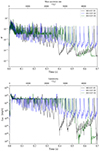 |
Fig. 1. Time evolution of mass accretion rate (̇M, upper panel) and luminosity (LBZ, lower panel) for the best models. |
4.2. Jet evolution
We analyzed the evolution of the simulated jets, focusing primarily on the best-fit models that closely match the observations of GRB 090510. Additionally, we discuss results from other models within our suite to provide a broader perspective on short GRB jet dynamics. As the accretion process onto the BH commences, the jet is launched almost instantaneously, driven by the rapid accumulation of magnetic flux and energy extraction mechanism at BH horizon. Figure 2 illustrates the density distribution of the accretion disk (top panels) and the jet structure (bottom panels) for selected models. The lower panels further depict the jet energy distribution using the μ parameter and the magnetization profiles represented by σ.
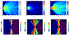 |
Fig. 2. Density distribution and jet structure at t = 0.3 seconds for three different models. Top row: Density plots of the accretion disk illustrating variations in the disk’s evolution across the three models. Bottom row: μ and σ parameters for each model, reflecting the jet energy distribution and magnetic field strength variations, respectively. |
Among all our models, the selected best-fit models that match the energetics and θj of GRB 090510 are MD-0.07-2D, DE1-0.07-2D, and DE2-0.07-2D. These models share similar parameters, except that the DE models incorporate an additional radially expanding DE component, as is described in Sect. 3.2.1. All three models exhibit comparable jet properties, with average opening angles of ⟨θj⟩ ≈ 9°−11°. The jet energy for these models ranges between Ejet = (1.1 − 1.60) × 1052 erg. The density profile and jet structure for the model MD-0.07-2D at 0.3 s is shown in the left panel of Fig. 2. The evolution of magnetic fields at three distinct times (0 s, 0.25 s, and 0.60 s) for this model is depicted through streamline plots in Figure 3, which effectively captures the dynamic changes in field topology. At t = 0, the left panel shows the initial poloidal field configuration. The middle panel represents the field setup at t = 0.25, during a stable accretion and jet phase, illustrating a well-defined magnetic structure. The right panel captures a later stage at t = 0.60, where the accretion process is partially obstructed, highlighting the complex threading of field lines in the vicinity of the BH.
 |
Fig. 3. Snapshots of disk density profile with magnetic field streamlines of model MD-0.07-2D at 0 s (left panel), 0.25 s (middle panel), and 0.60 s (right panel), respectively. |
Models DE1-0.07-2D and DE2-0.07-2D also have a very similar evolution in both density and jet profiles. These models were initialized with ejecta masses of 0.006 M⊙ and 0.012 M⊙, respectively, expanding radially with a constant velocity of 0.15c. We adopted ejecta masses and velocities within the lower limits reported in previous numerical studies (Radice et al. 2018; Gottlieb et al. 2022). All models assumed unmagnetized ejecta and a disk mass of 0.07 M⊙. In both cases, the resulting jet evolution shows no significant difference in dynamics compared to the model MD-0.07-2D, which lacks ejecta. The estimated opening angle, θj, remains nearly unchanged. This minimal impact is likely due to the fact that a substantial fraction of the ejecta exits the computational domain shortly after simulation begins. Considering η of 10% for the conversion of jet energy into radiation, these models can produce an average GRB energy (EGRB) on the order of ∼ 1.3 × 1051 erg, which is in close agreement with the collimation-corrected EGRB of GRB 090510. If we consider the value of η as 13.7%, 12.6%, and 9.5% for the models MD-0.07-2D, DE1-0.07-2D, and DE2-0.07-2D, respectively, we can produce the exact EGRB of 1.53 × 1051 ergs for GRB 090510.
In these models, one crucial factor that shapes the jets is the accretion disk winds – outflows of matter propelled outward by magnetic and thermal forces from the disk, significantly affecting the dynamics and emissions as the jet propagates away from the central engine. The temporal evolution of θj for these models is provided in Fig. 4. This shows how jet structure changes over time, on average.
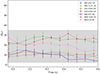 |
Fig. 4. Time evolution of the jet opening angle (θj) at 1000Rg for selected models. Both the angle and its standard deviation were computed at 0.05 s intervals to track temporal variations. For clarity, only a subset of the models is shown. The shaded gray region represents the range between the highest and lowest opening angle models, each extended by its respective standard deviation. |
Models LD1-0.003-2D and LD2-0.003-2D represent the low-density disk configurations in our sample. Although these models do not capture the specific observed properties of GRB 090510, they provide valuable insights into SGRB jet behavior under the assumption of a less dense accretion disk. The impact of disk winds on the structural changes in the jet for these models is minimal, which is evident from the density and jet structure shown in the middle panel of Fig. 2. This minimal impact of disk winds results in the largest θj (∼250) among all configurations in our study (see Table 2). Furthermore, the simulations for these models were run for over two seconds, demonstrating stability and producing a consistent luminosity on the order of 1049 erg s−1 until the end of the simulations.
The models HD1-0.60-2D and HD2-0.60-2D have the highest disk mass among our sample, accompanied by a highly turbulent and discontinuous jet structure throughout their lifetimes (see the right panel of Fig. 2 for the density and jet structure for the model HD1-0.60-2D at 0.3 seconds). Model HD2-0.60-2D also has the lowest plasma β among all our samples, producing a jet with a total energy of Ejet = 1.70 × 1053 erg, highest among our models. Notably, the most stable model with the lowest θj is MDC-0.08-2D, which has an FM torus with (Rin, Rmax) = (6, 11.5) Rg. This model represents the case with the closest distance between the initial torus and the BH in our study. Despite having a high plasma β of 2500, which was implemented to observe jet evolution over longer durations, this model produces a stable jet with an opening angle of θj ∼ 8° throughout its lifetime. This effect can be attributed to several key factors: a smaller disk radius results in a stronger interaction between the jet and disk winds, which collimates the jet at an earlier stage. Also, a high plasma-β environment reduces magnetic instabilities, allowing for a more stable jet structure, and the immediate jet-wind interaction at injection time helps maintain a narrow outflow. In contrast, when we attempt to increase the magnetic field strength to achieve a jet energy comparable to our target GRB, the jet becomes highly unstable. This suggests that while proximity to the BH aids collimation, achieving a balance between magnetic field strength and jet stability remains a key challenge for reproducing realistic GRB jets. The effect of disk geometry and other properties on jet structure and dynamics, especially in collimation, is discussed in detail in previous works (Christie et al. 2019; Hurtado et al. 2024).
In our sample, we have included one 3D model: HD-0.10-3D. This model was evolved until 0.6 seconds, yielding an average jet opening angle of θj ∼ 18°. The opening angle was estimated and averaged over each azimuthal (ϕ) slice. Although this value is higher than that observed for GRB 090510, the jet gradually collimates over time, reaching approximately θj ∼ 13° toward the end of the simulation. This collimated state of the jet from this model is shown by the 3D volume rendering map of jet magnetization, σ, in Fig. 5. From the results, we expect the jet to be more collimated with time. The three 2D models that we found to be most compatible with the observed target GRB also show a gradual increase in their collimation over time. On the other hand, HD models with strong magnetic fields and wind disturbances have no specific pattern and less predictable opening angle evolution.
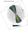 |
Fig. 5. Jet structure of 3D model in our sample, HD-0.10-3D. The parameter represented is jet magnetization σ, and the bounding box is 500 Rg. |
In total, we analyzed 11 models incorporating diverse initial simulation configurations, yielding jets with a broad range of observable properties. Table 2 provides an overview of all models, including their initial setups and average observable parameters. Our discussion here concentrates on selected models from each category, particularly those capable of reproducing the properties of GRB 090510.
4.3. Lorentz factor evolution
As discussed in Sect. 3.2.2, we calculated the terminal Lorentz factor, Γ∞, by taking the time average of μ. For selected models, we have presented the Γ∞ factor at different regions of the jet in Fig. 6. This visualization highlights the spatial variability of the Lorentz factor across the jets, underscoring the distinct behaviors and characteristics of each model’s jet structure. We can also observe the existence of a hollow core in the jets for an average angle of 3° −5°, which later gets closed over larger distances. Notably, our model MD-0.07-2D, which aligns closely with GRB 090510, exhibits Γ∞ factor estimates reaching as high as 375 at 3000 Rg and continues to increase with radius. The Γ∞ as a function of polar angle θ at a fixed radius of 3000 Rg for the MD models in the samples is provided in Fig. 7.
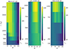 |
Fig. 6. Visualization of the Γ∞ distributions across different radii and angular ranges. The figure comprises three panels, each representing the Γ factor as a function of the radius (r) on the y axis and angle (θ) on the x axis for three different models. |
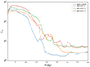 |
Fig. 7. Variation of Lorentz factor (Γ∞) as a function of polar angle θ for best-fit models, measured at a radius of 3000 Rg. |
4.4. Jet variability from simulations
In our simulations, the jet energetic parameter μ provides a measure of the total energy content of the jet. The time evolution of μ can give insights into the dynamics of processes within the jet that lead to variability, which we observe in the GRB LCs. Various studies have commented previously on jet variability from simulations (Tchekhovskoy et al. 2008; Lloyd-Ronning et al. 2016; Janiuk et al. 2021; James et al. 2022; Pais et al. 2024). We note that detailed calculations of the photospheric emission are needed to address the observed variability and nonthermal spectrum that arise in observations. However, even within the current setup, we are able to find hints of this variability in parameters such as μ and σ.
The time evolution of the μ parameter is provided in Fig. 8 at two different chosen locations (100 Rg, 8°), (150 Rg, 8°) for the model MD-0.07-2D. The parameter exhibits significant variability, which we use to investigate jet’s temporal evolution. Through our analysis of the μ parameter, we can compute the theoretical MTS, which is comparable with the MTS from observations, as is described in Sect. 2.2. By following the methodology described in Janiuk et al. (2021) and James et al. (2022), by computing the full width at half maximum for each discrete pulse and subsequently deriving a mean measure, we find variability timescales of 4.75 ms and 4.98 ms, respectively, in two locations [(100 Rg, 8°) and (150 Rg, 8°)] in the grid. These values are comparable to the estimated MTS for GRB 090510 from MacLachlan et al. (2013) using wavelet analysis, which is  ms. The comparison between the model and observations is within 1σ in both locations in the grid.
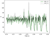 |
Fig. 8. Time evolution of the jet energetic parameter, μ, over time at two selected regions in the jet for the model MD-0.07-2D over which we have done the MTS calculations. |
4.5. Application to additional short GRBs
To demonstrate the broader applicability of our results beyond GRB 090510, we identified three additional short GRBs from the Fermi-GBM 10-year spectral catalog (Poolakkil et al. 2021) for which Eiso estimates are available and jet opening angles can be inferred using the method described in section 2.3. Redshift values for these bursts were taken from Gao et al. (2025). These GRBs are listed in Table 3, along with their Eiso, redshift, inferred θjet, and the best-matching simulation models from Table 2. The simulated and observed values show good agreement (within 10%), in terms of both energetics and opening angle. The collimation-corrected energies for these GRBs are also consistent with our models, based on Eq. (18) and when adopting the radiation efficiency in the range of 1–15%.
Jet opening angles and energetics for additional short GRBs used for comparison with our models.
To further explore the consistency of our models with jet parameters derived using independent methods, we included GRB 120804A in our comparison. This burst has an opening angle estimated from afterglow modeling (Fong et al. 2015). The derived θjet and energetics for this GRB are in close agreement with our simulated models. This reinforces that, for observationally reasonable angle estimates, our simulation framework can successfully reproduce key jet properties. This extended comparison illustrates that our simulation suite spans a realistic parameter space capable of reproducing not only GRB 090510 but also a broader population of short GRBs with similar jet properties.
5. Discussion
The primary goal of this work is to identify theoretical parameters that reproduce key observational features of the high-energy GRB 090510. To this end, we performed a suite of GRMHD simulations, focusing primarily on 2D runs. Additionally, we tested a single 3D configuration for completeness, though this preliminary attempt did not closely match the observed properties of GRB 090510. Given their significantly higher computational cost, the 3D simulations remain preliminary and are not the central focus of our present analysis. Instead, we base our conclusions largely on the 2D results, which provide an approximate range of jet properties for comparison with observational constraints.
However, in the literature as well, the discussion of theoretical models is hardly matched directly with observations due to the limited computational resources typically available. In this work, we mainly focus on matching the simulated energy and opening angle of the GRB jet, which exactly fits the observations within 1 σ (if we follow the efficiency level between 9.5–13.7%).
An important point to consider in the GRMHD simulations is the magnetic field strength and its initial configuration. This feature can directly shape the jet profile. Some authors consider toroidal fields in the initial state of the disk-jet simulation; for example Christie et al. (2019). Such fields must, however, originate from the NS merger system. The poloidal field that is adopted in our work is still in agreement with the outcome of numerical relativity simulations (Paschalidis et al. 2015; Sapountzis & Janiuk 2019).
Most of the models studied in this work required a high magnetization to produce targeted high jet luminosity. We find the existence of a magnetically arrested disk (MAD) state in these models. The MAD state strongly affects the creation of the outflow and the jet dynamics. In the 2D simulations, the evolution of magnetic fields is limited by the anti-dynamo theorem. The central engine’s time variability is strong but has highly periodic accretion cycles. These cycles lead to luminosity changes and quiescent intervals, and hence jet launching is sometimes suppressed. Since the non-axisymmetric instabilities (e.g., Rayleigh-Taylor, kink instabilities, see Bromberg et al. 2019) are suppressed, the jet emission is unstable. Therefore, the overall opening angle estimates in our analysis differ between the 2D and 3D simulations. In our simulations, the effect is prominent in HD models, while it seems to be lower in LD and MD models (they are in the standard and normal evolution (SANE) mode most of the time). In the 3D simulations, the MAD state is easily resolved, and we can observe the interchange instabilities or magnetic reconnections (Janiuk & James 2022; Nalewajko et al. 2024). This leads to a more efficient accretion and evolution of the accretion rate, reducing the amplitude of variability seen in 2D simulations.
The role of DE in shaping jet propagation has been highlighted in several recent studies. Analytical and numerical models suggest that the interaction with dense, radially expanding ejecta can lead to significant jet collimation on short timescales (Hamidani et al. 2020; Hamidani & Ioka 2020; Nagakura et al. 2014; Pais et al. 2023; Urrutia et al. 2025). In our simulations, however, this effect could not be confirmed due to computational limitations. The restricted radial extent of the simulation domain causes both the ejecta and the jet head to leave the grid within milliseconds of jet launching, preventing the formation of a stable collimation structure. While our setup provides a first-order test of DE influence, more extended simulations with larger domains and finer resolution will be required to fully capture its effect on jet evolution.
Continuing on our quest to match the observations and the theory, we have investigated the variability parameter. The time variability has been discussed in many avenues in the literature, both for GRBs and active galactic nuclei, and has been the subject of several definitions. Hence, there are different ways in which variability can be computed. As was already mentioned, it is beyond the scope of the current paper to discuss which method is more appropriate, but it is striking to observe that the calculation of the wavelet analysis is compatible with our simulations within 1σ. Given that the scope of the current paper is to test the reliability of this model and discuss its possible limitations, we focus on the main parameter, which is more univocally reproducible, such as the isotropic luminosity of the GRB, Liso, which is compatible within 1σ with our estimate. Indeed, our estimate of the observational bolometric luminosity (which is a proxy of the actual bolometric luminosity) was derived by summing the contribution of several wavelengths (high-energy γ-rays and X-rays).
Continuing the comparison with the observational properties, here we match our theoretical simulations with the observed θj. The observed θj still carries many uncertainties due to the density medium approximation used in these calculations. To avoid the use of any theoretical assumption, here we consider the method of Pescalli et al. (2015) to compare our simulated results with this estimate. In addition, following the discussion of Lloyd-Ronning et al. (2019a), the observations of θj of long GRBs (LGRBs) suggest that LGRB jets are narrower for those GRBs at higher redshift; thus, we consider this conclusion in this paper to compute more realistic estimates of θj. We have considered that SGRBs also undergo this evolution in our study, since luminosities for SGRBs and LGRBs evolve similarly (Dainotti et al. 2021; Petrosian & Dainotti 2024), and thus we have a similar expectation for the SGRBs. In the context of collimation by the stellar envelope, stars are generally characterized by lower metallicities at higher redshifts, which can collimate jets with greater efficiency. Although, in our calculation we have fixed the values to high spin to allow the energy to be high to match the observations, the effect of BH spin on the jet collimation angle for a magnetically launched jet for a range of spin values has been discussed (Hurtado et al. 2024). This means that, in principle, we can yet increase the spin to obtain a narrower jet, which would be consistent with the observed one even with a larger percentage of agreement. If we consider the evaluation of the θj method from Pescalli et al. (2015), we obtain θj = 6°; after we correct for redshift evolution, we reach a value of 10°.
Our analysis is primarily based on 2D simulations, supplemented by a single 3D model (HD-0.10-3D). Although 3D simulations can capture inherently 3D phenomena, such as magnetically arrested disk states and turbulence, more accurately, performing extensive parameter studies in high-resolution 3D setups remains computationally demanding. MAD states in 2D may induce artificial turbulence in jets, potentially leading to a slight underestimation of θjet. Furthermore, smoother accretion processes in 3D can yield marginally higher jet energetics compared to their 2D counterparts. Additionally, toroidal instabilities, which inherently require full 3D treatment, may further influence jet dynamics and energetics. In this context, Gottlieb et al. (2022) conducted a set of 3D GRMHD simulations to investigate jet behaviors in short GRBs. They identified jet “wobbling”, a toroidal instability causing periodic shifts in the jet direction. Such wobbling behavior can lead to intermittent emission peaks and variability in GRBs. This phenomenon is not observed in our current simulations, likely due to their limited evolution timescale. Despite these differences, our comprehensive 2D parameter study provides valuable insights into jet properties, capturing essential dynamics and yielding results that closely align with observational constraints for GRB 090510. Our findings thus set a viable foundation for future targeted high-resolution 3D investigations. In Kathirgamaraju et al. (2019), the simulated jet profile is analyzed. Similarly, from Fig. 7, which gives information on Γ∞, and Fig. 4, which provides the time evolution of θj, we can infer the jet structure. Specifically, Fig. 7 gives the average picture of the averaged jet profile over time at radii of 3000 Rg. However, in Fig. 4 we present the evolution of θj from the beginning, binned in 0.05 s, until 0.6 s.
Finally, in our numerical model, we do not implement neutrino cooling, whereas one must remember that this component should be taken into account in a physical model. In Fernández et al. (2019), the neutrino cooling effects are considered, and the authors show that the neutrino-driven winds can act as an additional collimation mechanism of the SGRB jet (see also, e.g. Urrutia et al. 2025). To check to what extent the DE have an impact on the θj, we added DE in our calculation following the same profile of Gottlieb et al. (2022), who added a specific profile of the medium behind the jet. They find the jet profile is changed, but they have a much extended computational grid.
6. Summary and conclusions
In this work, we have conducted detailed GRMHD simulations to investigate GRB 090510, a well-observed short GRB, across multiple wavelengths (De Pasquale et al. 2010; Fraija et al. 2016; Dainotti et al. 2021). Through simulations, we evaluated a range of values for θj within our model. We have found angles of a few degrees, which is not unusual, as is shown in the case of GRB 140903A (Troja et al. 2016). Subsequently, we compared these values with observed values obtained through alternative methods, such as the one detailed in Pescalli et al. (2015). Furthermore, we have explored the scalability of this model in terms of energy and redshift (z). From our numerical simulations, we determined the structure of the jet across the cone so that we go beyond the frequently used, simplified top-hat scenario. We also provided a physical model of the jet’s variable thermal and magnetic energy content and its ultimate Lorentz factor, Γ, estimations. Finally, we have linked the theoretically obtained jet properties with the ones determined for GRB 090510. While our primary analysis focused on GRB 090510, we also showed that the jet properties of several other short GRBs, including GRB 120804A with an opening angle independently constrained from afterglow observations, are consistent with our simulation models.
We highlight here that we reached the following takeaways:
-
The main drive for the jet collimation is represented by disk winds, with additional contributions from BH spin, magnetic field strength, and the proximity of the accretion disk.
-
We show that the three models are equally representative of the property of the burst and exhibit an average opening angle of 9.2°, 11.1°, and 10°. All these opening angles are compatible within 1 σ with the observed θj of 10.04° ±1.29° computed from the Pescalli et al. (2015) relation after correction for the jet evolution, considering that neither the Amati nor the Ghirlanda relation carries any uncertainties.
-
Similarly to the jet opening angle findings, we have observed compatibility of the variability values of 4.75 ms and 4.98 ms computed within two locations in the jet from our model and the wavelet analysis within 1σ as compared to the value of variability of
 discussed in MacLachlan et al. (2013).
 -
Although a single model cannot uniquely reproduce a specific GRB due to parameter degeneracies, our three models that match the observed EGRB do so with efficiencies ranging from η = 9.5 − 13.7%.
-
The model that has the smallest inner torus radii, placing it closest to the BH, produces a stable jet with the narrowest opening angle in all our models, consistent with the angle inferred for GRB 090510.
-
Three-dimensional simulations reveal a resolved MAD state that reduces variability and leads to smoother jet dynamics, enhancing our portrayal of realistic jet behavior in contrast to 2D models.
In conclusion, our work successfully achieves its primary goal of replicating the properties of a target GRB. By detailing various models in Table 2, we also set the stage for more extensive studies of GRB jets by setting up initial parameter ranges for future simulations. This integrated approach substantially advances our understanding of modeling high-energy GRBs.
The TS is defined as twice the logarithm of the ratio of the maximum likelihood obtained using a model including the GRB over the maximum likelihood value of the model that excludes the GRB.
When we apply the differential error propagation to derive the uncertainties in θj based on Eq. (8), namely on Eiso and on kA and kG we obtain a very large uncertainty of ±32° without redshift evolution correction. This source of uncertainties is large, and thus can lead to nonphysical values. In our comparison with the simulations, we refer to an ideal case of the Amati and Ghirlanda relation, which carries no uncertainties.
Acknowledgments
This work was supported by the grant 2019/35/B/ST9/04000 from the Polish National Science Center. A.J. was also partially supported by the NSC grant 2023/50/A/ST9/00527. We gratefully acknowledge Polish high-performance computing infrastructure PLGrid (HPC Center Cyfronet AGH) for providing computer facilities and support within computational grant no. PLG/2024/017347. We also thank Interdisciplinary Centre for Mathematical and Computational Modelling, University of Warsaw (ICM UW) for access to their resources. We acknowledge NAOJ’s support for hosting J.S. and A.J. during their visits at NAOJ. S.B. and M.G.D. acknowledge support from the Center for Computational Astrophysics at the National Astronomical Observatory of Japan, where part of the numerical computations were performed using the Cray XC50 supercomputer. We also thank Tomoya Takiwaki and Hiroki Nagakura for their useful suggestions and Asaf Peer and Gerardo Urrutia for the useful discussions.
References
- Ackermann, M., Asano, K., Atwood, W. B., et al. 2010, ApJ, 716, 1178 [NASA ADS] [CrossRef] [Google Scholar]
- Ajello, M., Arimoto, M., Axelsson, M., et al. 2019, ApJ, 878, 52 [NASA ADS] [CrossRef] [Google Scholar]
- Amati, L. 2014, AdP, 526, 340 [Google Scholar]
- Amati, L., Frontera, F., Tavani, M., et al. 2002, A&A, 390, 81 [NASA ADS] [CrossRef] [EDP Sciences] [Google Scholar]
- Amati, L., Frontera, F., & Guidorzi, C. 2009, A&A, 508, 173 [NASA ADS] [CrossRef] [EDP Sciences] [Google Scholar]
- Atwood, W. B., Abdo, A. A., Ackermann, M., et al. 2009, ApJ, 697, 1071 [CrossRef] [Google Scholar]
- Bauswein, A., Goriely, S., & Janka, H.-T. 2013, ApJ, 773, 78 [NASA ADS] [CrossRef] [Google Scholar]
- Beniamini, P., Nava, L., Duran, R. B., & Piran, T. 2015, MNRAS, 454, 1073 [NASA ADS] [CrossRef] [Google Scholar]
- Beniamini, P., Nava, L., & Piran, T. 2016, MNRAS, 461, 51 [NASA ADS] [CrossRef] [Google Scholar]
- Berger, E. 2014, ARA&A, 52, 43 [CrossRef] [Google Scholar]
- Bhat, P. N., Briggs, M. S., Connaughton, V., et al. 2012, ApJ, 744, 141 [NASA ADS] [CrossRef] [Google Scholar]
- Blandford, R. D., & Znajek, R. L. 1977, MNRAS, 179, 433 [NASA ADS] [CrossRef] [Google Scholar]
- Bloom, J. S., Frail, D. A., & Sari, R. 2001, ApJ, 121, 2879 [Google Scholar]
- Bloom, J. S., Frail, D. A., & Kulkarni, S. R. 2003, ApJ, 594, 674 [NASA ADS] [CrossRef] [Google Scholar]
- Bromberg, O., Singh, C. B., Davelaar, J., & Philippov, A. A. 2019, ApJ, 884, 39 [Google Scholar]
- Chevalier, R. A., & Li, Z.-Y. 2000, ApJ, 536, 195 [NASA ADS] [CrossRef] [Google Scholar]
- Christie, I. M., Lalakos, A., Tchekhovskoy, A., et al. 2019, MNRAS, 490, 4811 [NASA ADS] [CrossRef] [Google Scholar]
- Ciolfi, R. 2018, Int. J. Mod. Phys. D, 27, 1842004 [NASA ADS] [CrossRef] [Google Scholar]
- Corsi, A., Guetta, D., & Piro, L. 2010, ApJ, 720, 1008 [Google Scholar]
- Dainotti, M. G., Omodei, N., Srinivasaragavan, G. P., et al. 2021, ApJS, 255, 13 [Google Scholar]
- De Pasquale, M., Schady, P., Kuin, N. P. M., et al. 2010, ApJ, 709, L146 [NASA ADS] [CrossRef] [Google Scholar]
- Dessart, L., Ott, C. D., Burrows, A., Rosswog, S., & Livne, E. 2008, ApJ, 690, 1681 [Google Scholar]
- Efron, B., & Petrosian, V. 1992, ApJ, 399, 345 [NASA ADS] [CrossRef] [Google Scholar]
- Eichler, D. 2014, ApJ, 787, L32 [Google Scholar]
- Eichler, D., Livio, M., Piran, T., & Schramm, D. N. 1989, Nature, 340, 126 [NASA ADS] [CrossRef] [Google Scholar]
- Fan, Y., & Piran, T. 2006, MNRAS, 369, 197 [NASA ADS] [CrossRef] [Google Scholar]
- Fan, Y.-Z., & Wei, D.-M. 2011, ApJ, 739, 47 [Google Scholar]
- Fernández, R., Tchekhovskoy, A., Quataert, E., Foucart, F., & Kasen, D. 2019, MNRAS, 482, 3373 [CrossRef] [Google Scholar]
- Fishbone, L. G., & Moncrief, V. 1976, ApJ, 207, 962 [NASA ADS] [CrossRef] [Google Scholar]
- Fong, W., Berger, E., Margutti, R., & Zauderer, B. A. 2015, ApJ, 815, 102 [NASA ADS] [CrossRef] [Google Scholar]
- Fong, W., Laskar, T., Rastinejad, J., et al. 2021, ApJ, 906, 127 [NASA ADS] [CrossRef] [Google Scholar]
- Foucart, F., Duez, M. D., Kidder, L. E., Pfeiffer, H. P., & Scheel, M. A. 2024, PRD, 110, 024003 [Google Scholar]
- Fraija, N., Lee, W. H., Veres, P., & Barniol Duran, R. 2016, ApJ, 831, 22 [NASA ADS] [CrossRef] [Google Scholar]
- Frail, D. A., Kulkarni, S. R., Sari, R., et al. 2001, ApJ, 562, L55 [NASA ADS] [CrossRef] [Google Scholar]
- Gammie, C. F., McKinney, J. C., & Tóth, G. 2003, ApJ, 589, 444 [Google Scholar]
- Gao, W.-H., Mao, J., Xu, D., & Fan, Y.-Z. 2009, ApJ, 706, L33 [Google Scholar]
- Gao, C. Y., Wei, J. J., & Zeng, H. D. 2025, Constraining the Luminosity Function and Delay-Time Distribution of Short Gamma-Ray Bursts for Multimessenger Gravitational-Wave Detection Rate Estimation [Google Scholar]
- Ghirlanda, G., Ghisellini, G., & Lazzati, D. 2004, ApJ, 616, 331 [Google Scholar]
- Ghirlanda, G., Nava, L., Ghisellini, G., & Firmani, C. 2007, A&A, 466, 127 [NASA ADS] [CrossRef] [EDP Sciences] [Google Scholar]
- Goldstein, A., Connaughton, V., Briggs, M. S., & Burns, E. 2016, ApJ, 818, 18 [CrossRef] [Google Scholar]
- Golkhou, V. Z., Butler, N. R., & Littlejohns, O. M. 2015, ApJ, 811, 93 [NASA ADS] [CrossRef] [Google Scholar]
- Gompertz, B. P., Levan, A. J., Tanvir, N. R., et al. 2018, ApJ, 860, 62 [NASA ADS] [CrossRef] [Google Scholar]
- Gottlieb, O., Moseley, S., Ramirez-Aguilar, T., et al. 2022, ApJ, 933, L2 [NASA ADS] [CrossRef] [Google Scholar]
- Hamidani, H., & Ioka, K. 2020, MNRAS, 500, 627 [NASA ADS] [CrossRef] [Google Scholar]
- Hamidani, H., Kiuchi, K., & Ioka, K. 2020, MNRAS, 491, 3192 [NASA ADS] [Google Scholar]
- He, H.-N., Wu, X.-F., Toma, K., Wang, X.-Y., & Mészáros, P. 2011, ApJ, 733, 22 [Google Scholar]
- Hotokezaka, K., Kiuchi, K., Kyutoku, K., et al. 2013a, PRD, 88, 044026 [Google Scholar]
- Hotokezaka, K., Kiuchi, K., Kyutoku, K., et al. 2013b, PRD, 87, 024001 [Google Scholar]
- Hurtado, V. U., Lloyd-Ronning, N. M., & Miller, J. M. 2024, ApJ, 967, L4 [Google Scholar]
- James, B., Janiuk, A., & Nouri, F. H. 2022, ApJ, 935, 176 [NASA ADS] [CrossRef] [Google Scholar]
- Janiuk, A., & James, B. 2022, A&A, 668, A66 [NASA ADS] [CrossRef] [EDP Sciences] [Google Scholar]
- Janiuk, A., James, B., & Palit, I. 2021, ApJ, 917, 102 [NASA ADS] [CrossRef] [Google Scholar]
- Jin, Z.-P., Covino, S., Liao, N.-H., et al. 2020, Nat. Astron., 4, 77 [NASA ADS] [CrossRef] [Google Scholar]
- Kathirgamaraju, A., Tchekhovskoy, A., Giannios, D., & Barniol Duran, R. 2019, MNRAS, 484, L98 [CrossRef] [Google Scholar]
- Kobayashi, S., & Sari, R. 2001, ApJ, 551, 934 [NASA ADS] [CrossRef] [Google Scholar]
- Kobayashi, S., Piran, T., & Sari, R. 1997, ApJ, 490, 92 [Google Scholar]
- Kouveliotou, C., Meegan, C. A., Fishman, G. J., et al. 1993, ApJ, 413, L101 [NASA ADS] [CrossRef] [Google Scholar]
- Kumar, P., & Zhang, B. 2015, Phys. Rep., 561, 1 [Google Scholar]
- Levan, A. 2018, Gamma-Ray Bursts (IOP Publishing), 2514 [Google Scholar]
- Lien, A., Sakamoto, T., Barthelmy, S. D., et al. 2016, ApJ, 829, 7 [Google Scholar]
- Lloyd-Ronning, N. M., & Zhang, B. 2004, ApJ, 613, 477 [NASA ADS] [CrossRef] [Google Scholar]
- Lloyd-Ronning, N. M., Dolence, J. C., & Fryer, C. L. 2016, MNRAS, 461, 1045 [Google Scholar]
- Lloyd-Ronning, N. M., Aykutalp, A., & Johnson, J. L. 2019a, MNRAS, 488, 5823 [NASA ADS] [CrossRef] [Google Scholar]
- Lloyd-Ronning, N. M., Fryer, C., Miller, J. M., et al. 2019b, MNRAS, 485, 203 [NASA ADS] [CrossRef] [Google Scholar]
- Lloyd-Ronning, N. M., Johnson, J. L., & Aykutalp, A. 2020, MNRAS, 498, 5041 [NASA ADS] [CrossRef] [Google Scholar]
- Lu, R.-J., Wei, J.-J., Qin, S.-F., & Liang, E.-W. 2012, ApJ, 745, 168 [Google Scholar]
- MacFadyen, A. I., & Woosley, S. E. 1999, ApJ, 524, 262 [NASA ADS] [CrossRef] [Google Scholar]
- MacLachlan, G. A., Shenoy, A., Sonbas, E., et al. 2013, MNRAS, 432, 857 [NASA ADS] [CrossRef] [Google Scholar]
- Meegan, C., Lichti, G., Bhat, P. N., et al. 2009, ApJ, 702, 791 [Google Scholar]
- Metzger, B. D. 2017, Liv. Rev. Relativ., 20, 3 [NASA ADS] [CrossRef] [Google Scholar]
- Metzger, B. D., Giannios, D., Thompson, T. A., Bucciantini, N., & Quataert, E. 2011, MNRAS, 413, 2031 [Google Scholar]
- Nagakura, H., Hotokezaka, K., Sekiguchi, Y., Shibata, M., & Ioka, K. 2014, ApJ, 784, L28 [CrossRef] [Google Scholar]
- Nalewajko, K., Kapusta, M., & Janiuk, A. 2024, A&A, 692, A37 [NASA ADS] [CrossRef] [EDP Sciences] [Google Scholar]
- Nativi, L., Lamb, G. P., Rosswog, S., Lundman, C., & Kowal, G. 2021, MNRAS, 509, 903 [NASA ADS] [CrossRef] [Google Scholar]
- Nedora, V., Bernuzzi, S., Radice, D., et al. 2021, ApJ, 906, 98 [NASA ADS] [CrossRef] [Google Scholar]
- Nicuesa, G. A., Klose, S., Greiner, J., et al. 2012, A&A, 548, A101 [NASA ADS] [CrossRef] [EDP Sciences] [Google Scholar]
- Noble, S. C., Gammie, C. F., McKinney, J. C., & Zanna, L. D. 2006, ApJ, 641, 626 [NASA ADS] [CrossRef] [Google Scholar]
- Oechslin, R., Janka, H.-T., & Marek, A. 2007, A&A, 467, 395 [NASA ADS] [CrossRef] [EDP Sciences] [Google Scholar]
- Paczynski, B. 1986, ApJ, 308, L43 [NASA ADS] [CrossRef] [Google Scholar]
- Pais, M., Piran, T., Lyubarsky, Y., Kiuchi, K., & Shibata, M. 2023, ApJ, 946, L9 [Google Scholar]
- Pais, M., Piran, T., Kiuchi, K., & Shibata, M. 2024, ApJ, 976, 35 [Google Scholar]
- Panaitescu, A. 2011, MNRAS, 414, 1379 [NASA ADS] [CrossRef] [Google Scholar]
- Paschalidis, V., Ruiz, M., & Shapiro, S. L. 2015, ApJ, 806, L14 [NASA ADS] [CrossRef] [Google Scholar]
- Pavan, A., Ciolfi, R., Kalinani, J. V., & Mignone, A. 2021, MNRAS, 506, 3483 [CrossRef] [Google Scholar]
- Pescalli, A., Ghirlanda, G., Salafia, O. S., et al. 2015, MNRAS, 447, 1911 [NASA ADS] [CrossRef] [Google Scholar]
- Petrosian, V., & Dainotti, M. G. 2024, ApJ, 963, L12 [Google Scholar]
- Pian, E., Mazzali, P. A., Masetti, N., et al. 2006, Nature, 442, 1011 [Google Scholar]
- Poolakkil, S., Preece, R., Fletcher, C., et al. 2021, ApJ, 913, 60 [NASA ADS] [CrossRef] [Google Scholar]
- Radice, D., Perego, A., Hotokezaka, K., et al. 2018, ApJ, 869, 130 [Google Scholar]
- Rastinejad, J. C., Fong, W., Kilpatrick, C. D., Nicholl, M., & Metzger, B. D. 2024, Uniform Modeling of Observed Kilonovae: Implications for Diversity and the Progenitors of Merger-Driven Long Gamma-Ray Bursts [Google Scholar]
- Rosswog, S., Ramirez-Ruiz, E., & Davies, M. B. 2003, MNRAS, 345, 1077 [Google Scholar]
- Ruffini, R., Muccino, M., Aimuratov, Y., et al. 2016, ApJ, 831, 178 [Google Scholar]
- Salafia, O. S., & Ghirlanda, G. 2022, Galaxies, 10, 5 [Google Scholar]
- Sapountzis, K., & Janiuk, A. 2019, ApJ, 873, 12 [NASA ADS] [CrossRef] [Google Scholar]
- Sari, R., & Piran, T. 1997, ApJ, 485, 270 [NASA ADS] [CrossRef] [Google Scholar]
- Sari, R., Piran, T., & Halpern, J. P. 1999, ApJ, 519, L17 [NASA ADS] [CrossRef] [Google Scholar]
- Scargle, J. D., Norris, J. P., Jackson, B., & Chiang, J. 2013, ApJ, 764, 167 [Google Scholar]
- Sekiguchi, Y., Kiuchi, K., Kyutoku, K., & Shibata, M. 2011, PRL, 107, 051102 [Google Scholar]
- Soderberg, A. M., Kulkarni, S. R., Nakar, E., et al. 2006, Nature, 442, 1014 [CrossRef] [Google Scholar]
- Tchekhovskoy, A., McKinney, J. C., & Narayan, R. 2008, MNRAS, 388, 551 [NASA ADS] [CrossRef] [Google Scholar]
- Troja, E., Sakamoto, T., Cenko, S. B., et al. 2016, ApJ, 827, 102 [Google Scholar]
- Urrutia, G., DeColle, F., Murguia-Berthier, A., & Ramirez-Ruiz, E. 2021, MNRAS, 503, 4363 [CrossRef] [Google Scholar]
- Urrutia, G., Janiuk, A., & Hossein Nouri, F. 2025, MNRAS, 538, 1247 [Google Scholar]
- Valenti, S., Sand, D. J., Yang, S., et al. 2017, ApJ, 848, L24 [CrossRef] [Google Scholar]
- Vlahakis, N., & Königl, A. 2003, ApJ, 596, 1080 [NASA ADS] [CrossRef] [Google Scholar]
- Watson, D., Hjorth, J., Jakobsson, P., et al. 2006, A&A, 454, L123 [NASA ADS] [CrossRef] [EDP Sciences] [Google Scholar]
All Tables
Jet opening angles and energetics for additional short GRBs used for comparison with our models.
All Figures
|
Fig. 1. Time evolution of mass accretion rate (̇M, upper panel) and luminosity (LBZ, lower panel) for the best models. |
| In the text | |
|
Fig. 2. Density distribution and jet structure at t = 0.3 seconds for three different models. Top row: Density plots of the accretion disk illustrating variations in the disk’s evolution across the three models. Bottom row: μ and σ parameters for each model, reflecting the jet energy distribution and magnetic field strength variations, respectively. |
| In the text | |
|
Fig. 3. Snapshots of disk density profile with magnetic field streamlines of model MD-0.07-2D at 0 s (left panel), 0.25 s (middle panel), and 0.60 s (right panel), respectively. |
| In the text | |
|
Fig. 4. Time evolution of the jet opening angle (θj) at 1000Rg for selected models. Both the angle and its standard deviation were computed at 0.05 s intervals to track temporal variations. For clarity, only a subset of the models is shown. The shaded gray region represents the range between the highest and lowest opening angle models, each extended by its respective standard deviation. |
| In the text | |
|
Fig. 5. Jet structure of 3D model in our sample, HD-0.10-3D. The parameter represented is jet magnetization σ, and the bounding box is 500 Rg. |
| In the text | |
|
Fig. 6. Visualization of the Γ∞ distributions across different radii and angular ranges. The figure comprises three panels, each representing the Γ factor as a function of the radius (r) on the y axis and angle (θ) on the x axis for three different models. |
| In the text | |
|
Fig. 7. Variation of Lorentz factor (Γ∞) as a function of polar angle θ for best-fit models, measured at a radius of 3000 Rg. |
| In the text | |
|
Fig. 8. Time evolution of the jet energetic parameter, μ, over time at two selected regions in the jet for the model MD-0.07-2D over which we have done the MTS calculations. |
| In the text | |
Current usage metrics show cumulative count of Article Views (full-text article views including HTML views, PDF and ePub downloads, according to the available data) and Abstracts Views on Vision4Press platform.
Data correspond to usage on the plateform after 2015. The current usage metrics is available 48-96 hours after online publication and is updated daily on week days.
Initial download of the metrics may take a while.