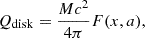
| Issue |
A&A
Volume 702, October 2025
|
|
|---|---|---|
| Article Number | A272 | |
| Number of page(s) | 20 | |
| Section | Astrophysical processes | |
| DOI | https://doi.org/10.1051/0004-6361/202554222 | |
| Published online | 28 October 2025 | |
A Monte Carlo spectropolarimetric model for the high-soft state of neutron star low-mass X-ray binaries
1
INAF – Osservatorio di Astrofisica e Scienza dello Spazio di Bologna, Via P. Gobetti 101, I-40129 Bologna, Italy
2
INAF – Osservatorio Astronomico di Cagliari, Via della Scienza 5, I-09047 Selargius (CA), Italy
⋆ Corresponding author: This email address is being protected from spambots. You need JavaScript enabled to view it.
Received:
21
February
2025
Accepted:
4
August
2025
Abstract
Context. After a few years of X-ray polarimetric astrophysics provided by the IXPE space observatory, the knowledge of the physics and geometry of weakly magnetized neutron star X-ray binaries is newly increasing both in quantity and quality terms. Energy resolved polarimetry is thus an undoubtedly powerful tool to investigate the accretion properties of this class of objects. While numerical spectropolarimetric codes of black hole X-ray binaries, whose results can be compared with observations, are available to the research, similar tools for neutron star systems still must be developed.
Aims. This work is part of an ambitious project aimed at providing the scientific community with a series of models for spectropolarimetric studies of binary systems containing neutron stars in different spectral states.
Methods. We developed a new Monte Carlo radiative transfer ray-tracing code in which both quantum mechanics and general relativity effects are fully taken into account and accurate counting statistics for the spectra are obtained by parallel computing on multi-core clusters. The model was built in the framework of an accretion disk plus boundary layer scenario specifically focused on the high-soft state of neutron star low-mass X-ray binaries. We applied the code to build a tabular spectroscopic model for the XSPEC package and fit the NuSTAR and IXPE spectra of the Z source Cyg X-2 and the bright atoll source GX 9+9.
Results. The new model successfully fits the source spectra and predicts a dependence with energy of the polarization degree and polarization angle consistent with observations. Further updates will be implemented in the future to study the challenging cases of polarimetric behavior suggesting accretion geometries different from those with azimuthal symmetry.
Key words: accretion, accretion disks / radiation mechanisms: general / radiative transfer / relativistic processes
© The Authors 2025
 Open Access article, published by EDP Sciences, under the terms of the Creative Commons Attribution License (https://creativecommons.org/licenses/by/4.0), which permits unrestricted use, distribution, and reproduction in any medium, provided the original work is properly cited.
This article is published in open access under the Subscribe to Open model. This email address is being protected from spambots. You need JavaScript enabled to view it. to support open access publication.
1. Introduction
Within the astrophysical domain, the exploration of X-ray binaries (XRBs) hosting a compact object unveils a paradigmatic avenue into the cosmic phenomena of compact objects and offers a captivating window from which to study physical processes in the strong gravity regime. The physics of these systems has been long investigated through spectral and temporal studies; however, there are still several unanswered questions (for a review, see Done et al. 2007).
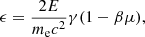
A sub-class of the most general XRB population contains main sequence stars, with M ≲ M⊙ orbiting around a weakly magnetized neutron star (NS) with B ≲ 108 − 9 G, the so-called low-mass X-ray binaries (LMXBs). These systems have historically been divided into two further sub-classes, the Z and atoll sources (Hasinger & van der Klis 1989), on the basis of their temporal pattern in the color-color or color-intensity diagram. In their brightest, high accretion regimes – the high-soft state (HSS) – the spectra of LMXBs are usually described by a two-component model consisting of a Comptonization feature at higher energies plus softer thermal emission attributed either to the accretion disk (e.g., Mitsuda et al. 1989; Di Salvo et al. 2000, 2001; Lavagetto et al. 2004; Farinelli et al. 2008, 2009; Navale et al. 2024) or to a blackbody (BB) at temperature kTbb ∼ 1.5 keV coming from the NS (White et al. 1988; Iaria et al. 2020). The two scenarios were labeled as the Eastern Model (EM) and Western Model (WM), respectively. The analysis of a sample of atoll and Z sources using Fourier frequency-resolved spectroscopy revealed that the unsaturated Comptonization component can be described in terms of a spreading layer (SL) around the NS with a power spectrum resembling the Fourier frequency-resolved spectrum at the period of quasi-periodic oscillations (Gilfanov et al. 2003; Revnivtsev & Gilfanov 2006; Revnivtsev et al. 2013). In many cases, in addition to the persistent two-component continuum, a reflection feature attributable to a fully or partially ionized accretion disk has been detected in both Z and bright atoll sources (Piraino et al. 1999; Mondal et al. 2019; Iaria et al. 2020; Ludlam et al. 2022). An important difference from the spectral point of view between the two classes is that all known Z sources (Cyg X-2, GX 5-1, GX 340+0, Sco X-1, GX 17+2 and GX 349+2) always remain in HSS, where the Comptonization component has a low temperature (kTe ∼ 3 keV) and high optical depth τ ∼ 5–10, depending on the assumption of plasma geometry (slab-like or spherical).
Atoll sources, on the other hand, can be divided into two further sub-classes. Sources of the first class (GX 13+1, GX 3+1, GX 9+9, GX 9+1) have only been observed in the HSS, while the others may experience a state transition from HSS to low-hard state (LHS), which is characterized by a dimmer flux in the X-ray band and a significantly harder spectrum, where the electron temperature can achieve about 30 keV, in a low optical depth environment (e.g., Guainazzi et al. 1998; Paizis et al. 2006; Falanga et al. 2006; Cocchi et al. 2010). Conversely, several sources, mainly type I X-ray bursters, are predominantly observed in their LHS. The first link between Z and atoll sources was found with the observation of the outburst of the peculiar transient XTE J1701-462 (Remillard et al. 2006). It is a rather unique object that experienced all the known spectral states of the NS-LMXB during its 2006 outburst (Lin et al. 2009).
A unique opportunity to unveil the accretion geometry of NS-LMXBs has come with the launch of the Imaging X-ray Polarimetry Explorer (IXPE; Weisskopf et al. 2016) on December 9, 2021. Because of their brightness, NS-LMXBs have been among the preferred targets of the IXPE observational campaigns so far; however, sources only in the HSS could be studied with some statistical accuracy (Ursini et al. 2024; Gnarini et al. 2025).
From a purely phenomenological perspective, what has been observed so far is that for Z sources, the polarization degree (PD) is higher in the horizontal branch (HB) and progressively decreases toward the normal branch (NB). This trend was clearly observed in the 2022 outburst of XTE J1701−462 (Cocchi et al. 2010; Jayasurya et al. 2023) and in GX 5-1 (Fabiani et al. 2024), with a PD ∼4 − 5% in the HB that decreased down to ≲2% either in the NB or, in the case of GX 5-1, down to the apex connecting the NB with the flaring branch (FB). The low PD value (∼1%) measured in Sco X-1 while the source was at the NB-FB apex is consistent with this trend (La Monaca et al. 2024a). For GX 340+0, a PD of ∼4% was measured when the source was in the HB (La Monaca et al. 2024b), while for Cyg X-2 Farinelli et al. (2023, hereafter F23) found a PD of ∼1.8% with the source in the NB. It is interesting to note that for GX 349+2, Kashyap et al. (2025) measured a higher PD in the FB than in the NB, thus almost contradicting what previously appeared to be a monotonic trend along the Z track.
Evidence of an increase of PD with energy has been found for Cyg X-2, XTE J1701−462, GX 5-1, GX 340+0, GX 349+2, and Sco X-1 (Long et al. 2022) as well as for GX 9+9 (Ursini et al. 2023, hereafter U23), 4U 1624-49 (Saade et al. 2024; Gnarini et al. 2024a), and 4U 1820-303 (Di Marco et al. 2023). The feature therefore appears to be shared by both Z and atoll sources.
The behavior of the polarization angle (PA) is another challenging element for data interpretation. For Cyg X-2, the 2–8 keV PA was found to be roughly aligned with the position of the radio jet, which is similar to what was found for Sco X-1 with Polarlight. Moreover, the data showed a hint of a swap between the PAs of the soft and hard components, which were fixed at 90° to each other. Compared to PolarLight observations, the 2–8 keV PA of Sco X-1 measured by IXPE was found to be rotated by about 50° with respect to the value reported by Long et al. (2022). For GX 5-1, a rotation of the PA with energy of about 20° was reported by Fabiani et al. (2024) by averaging data from all observations, whose more natural explanation is the presence of a warped disk. Despite being the second-brightest source of the X-ray sky, data statistics did not allow for investigation of the energy-dependent PA behavior across different positions of the Z track. For Cir X-1, IXPE measured a change of PA of about ∼50° across different intervals of the orbital phase, with a quasi constant PD around ∼1.5% (Rankin et al. 2024), while in GX 13+1, the variation of both the PD and PA (with a rotation up to ∼50°) with time have been reported (Bobrikova et al. 2024). In GX 340+0, the PA of the soft and hard components were found to be misaligned by 40°.
Another critical aspect of the present IXPE legacy is the estimation of the contribution to the net polarization signal provided by different regions of NS-LMXBs. The difficulty in disentangling single components becomes evident when noticing that to date only upper limits have been placed on the PD of the disk, which actually prevent any serious constraint regarding physical conditions of the disk atmosphere from polarimetry from being placed. Concerning the harder component, the highest value of the PD (up to ∼4–5%) has been attributed to the Comptonization component, but this often appears to be an artifact due to inverse Compton occurring in a boundary layer (BL) roughly perpendicular to the disk that has its PA aligned to that of the reflected component (Schnittman & Krolik 2009), which is likely responsible for the high observed PD.
We emphasize that in the literature, the terms SL and BL are often used interchangeably, which can lead to confusion. From this point onward in the paper, we consider them equivalent, referring to the BL/SL as the sub-Keplerian transition region between the inner disk and the NS surface, with a radial extension smaller than the polar one.
2. The status of theory in X-ray polarimetry
Despite the theory of radiative transfer for polarized radiation dating back to Chandrasekhar (1960), there are very few models attempting to predict the PD in NS-LMXBs. In this context, the seminal work of Lapidus & Sunyaev (1985) deserves to be outlined, which for the BL plus reflection component of X-ray bursters derived a PD up to 6% during the out-of-burst phase. However, numerical results via Monte Carlo (MC) simulations have been reported only recently using the code MONK by Gnarini et al. (2022). The main problem in this latter case consists not only in the fact that disk reflection was not included (likely introducing a systematic bias in the results) but also that results were presented for a handful of configurations with standard parameters for the soft and hard state using naive geometries, with some subsequent updated configuration for the Comptonized component (Capitanio et al. 2023).
The polarization properties of the BL have been studied by Farinelli et al. (2024, hereafter F24) and Bobrikova et al. (2025, hereafter B25), and in both cases it was found that the PD does not exceed about 1.5%. The fact that both groups independently obtained the same result is undoubtedly reassuring, as it places stringent constraints on the spectropolarimetric properties of the hard component, suggesting that the dominant part of the polarized signal presumably comes from reflection of the BL radiation by the disk surface.
Most of the theoretical efforts are focused in computing spectropolarimetry of radiation coming from the accretion disk, implicitly or explicitly assuming a black hole (BH) as central compact object (Sunyaev & Titarchuk 1985, hereafter ST85; Poutanen & Svensson 1996; Schnittman & Krolik 2010; Dovčiak et al. 2011; Podgorný et al. 2022; Loktev et al. 2022), and for polar caps of accreting millisecond X-ray pulsars (Viironen & Poutanen 2004; Poutanen 2020).
The lack of thorough numerical codes to perform modeling of the spectropolarimetric properties of NS LMXBs may originate from the fact that if from one side general relativity is fundamental to obtain realistic results in strong gravity regimes, from the other while for BH systems the Einstein field equations have exact solutions (the Schwarzschild or Kerr metric) and efforts are focused essentially on the accretion disk physics, for NS systems the geometry and hydrodynamical configuration may be rather complex, with at least two different sources of seed photons which must be correctly cross-normalized and coupled with a tracking of photons potentially traveling from the BL to the disk and backward.
However, the current IXPE legacy makes no longer postponeable the development of as most as possible detailed numerical codes which are fundamental in the data interpretation.
In particular, MC codes appear to be the only viable way to produce theoretical results in which both general relativity and quantum mechanics are self-consistently taken into account. A trade-off between complexity and computational time is nevertheless needed: for instance, Taverna et al. (2021, hereafter T21) studied the polarimetric properties of radiation from a relativistic accretion disk (Page & Thorne 1974, hereafter PT74) by coupling a former computation of the matter thermodynamical properties with the code CLOUDY (Ferland et al. 2017), and later used this as an input for the code STOKES (Goosmann & Gaskell 2007; Marin et al. 2012). The outputs, albeit detailed, are computed in the static rest frame, so a convolution with the disk velocity profile as well as light bending effects would be needed to derive polarization parameters in the observer frame. In general, theoretical works present results for a handful of combinations of the physical and geometrical parameters used to develop a model (Schnittman & Krolik 2013; Abarr & Krawczynski 2020; Gnarini et al. 2022; Poutanen et al. 2023). What would be highly desirable is to have models capable of fitting the spectropolarimetric data of sources using packages such as XSPEC (Arnaud 1996). This task is undoubtedly challenging, as models that calculate Stokes parameters (I, Q, U) at runtime must rely on unavoidable simplifications to keep computation times reasonable. The alternative is to create tabular models based on MC simulations. The drawback of MC simulations is the requirement of high-performance computing infrastructures to generate statistically robust layouts that can then be incorporated into tabular grids. The situation becomes even more critical when, in addition to flux spectra, one aims to produce Q and U spectra. This requires an even higher number of photons to avoid statistical fluctuations that would prevent the proper tracking of the energy-dependence behavior of the latter two quantities, allowing them to be suitable for data fitting once stored in the grids.
In this paper, we present a new MC ray-tracing algorithm aimed at simulating the spectropolarimetric layout of NS-LMXBs in HSS. Using a series of post-simulation scripts, we then created a tabular model for the XSPEC package, specifically designed to fit the Stokes (I, Q, U) spectra of these sources. This work is part of a long-term project aimed at releasing to the astrophysical community a series of tabular models to be used for the study of XRBs hosting either a NS or a BH in different spectral states. The tabular model we present here, and which we label as bldisk according to XSPEC therminology, was built from MC simulations specifically for the HSS of bright NS-LXMBs, no matter the subclass they belong to. The paper is structured as follows: in Sect. 3 we report a detailed description of the mathematical and physical formalism which has been implemented to build the MC code, while in Sect. 4 we describe the specific setup we used to characterize the spectropolarimetric layout. In Sect. 5, we show spectroscopic applications of bldisk to two sources of the Z and bright atoll class, comparing the inferred theoretical polarimetry to observational results obtained by IXPE. The physical implications as well as model specific range of applicability are discussed in Sect. 6, while final conclusions are drawn in Sect. 7.
3. Physics of the ray-tracing algorithm
The code has been written in C-language and uses the GNU Scientific Libary (GSL)1 for ad hoc mathematic computing. It is designed for a photon-by-photon tracking, so that each generated photon is followed once at time. To increase the statistics of the output results, the code performs parallel runs by mean of the Message Passing Interface (MPI) library. More specifically, a single run with 𝒩γ photons on ℳc cores results in a total of 𝒩γ × ℳc generated photons. Then, the higher the number of computing cores, the better is the output statistics for a given single-core group of photons. The simulated spectra to create the bldisk grid have been obtained with a total of 1.25 × 10⁷ photons for each grid point.
Our technique differs from that implemented in other simulators such as MONK (Zhang et al. 2019) and GRMONTY (Dolence et al. 2009), which are based on the photon-packages techinique, also called “superphotons” (Pozdnyakov et al. 1983). On the other hand, the photon-by photon project STOKES works in Thomson scattering regime, and does not include general relativity effects.
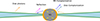 |
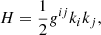
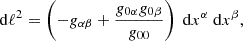
Fig. 1. Geometrical setup for the bldisk model. Blackbody seed photons from the neutron star are Comptonized in a boundary layer extending up to some latitude (orange region) and characterized by a given electron temperature kTe and optical depth τbl. The other source of thermal photons is the accretion disk, where seed photons are emitted at the top of an electron-scattering atmosphere of optical depth τdisk (green region). Some photons from the disk are Comptonized by the boundary layer, and in turn, the radiation emitted from the latter reaches the disk atmosphere and gets reflected. |
3.1. Integration of Hamilton-Jacoby equations
We consider a Kerr spacetime around the rotating NS, in which the spin parameter is related to the NS period by a = 0.47/P (Braje et al. 2000), where P is the period in milliseconds. The metric tensor in Boyer-Lindquist coordinates is (Landau & Lifshitz 1975)
 (1)
(1)
where the non-zero components with the metric signature ( + − − − ) are
 (2a)
(2a)
 (2b)
(2b)
 (2c)
(2c)
 (2d)
(2d)
 (2e)
(2e)
with Σ2 = r2 + a2cos2θ and Δ = r2 − rrs + a2. It is worth noticing that with this formalism rs is the Schwarzschild radius (i.e., twice the gravitational radius) and the spin is defined such that |a|< 0.5, so a multiplication factor 1/2 must be used in the above formula relating it with the NS period.
The photon trajectory across geodesics are obtained by solving the coupled Hamilton-Jacoby equations (Levin & Perez-Giz 2008):
 (3a)
(3a)
 (3b)
(3b)
where the Hamiltonian is defined as
 (4)
(4)
while xi and ki are the photon four-position and covariant four-momentum respectively. The integration of Eqs. (3a) and (3b) is performed through the adimensional affine parameter λ which is set equal to zero at the photon initial position and then progressively increases.
Another differential equation to be integrated is the one required to compute the optical depth while photons propagate in the medium, according to
 (5)
(5)
where Rs is Schwarzschild radius of the compact object, ui the matter four-velocity and α(E) the absorption coefficient for photon with energy E in the matter rest frame, computed at the given position (Younsi et al. 2012).
The critical plasma density above which free-free absorption becomes competing with Compton scattering is (Pozdnyakov et al. 1983)
 (6)
(6)
where g(x) is the Gaunt factor and x ≡ E/kTe. For kTe∼ 5 keV, Nc ranges from ∼5 × 1023 cm−3 at E = 2 keV, to ∼8 × 1025 cm−3 at E = 8 keV, and it is easy to show that electron densities of the BL and disk atmosphere in the range of parameters defined to build bldisk are much lower than these, so that electron scattering dominates over free-free absorption, and results in the IXPE band are not affected at all. The coefficients becomes approximately comparable only for E ≲ 0.2 keV, and at the present stage we only consider Compton scattering, for which the absorption coefficient is
 (7)
(7)
where ne(γ) is a normalized fluid frame electron distribution, N0 the total electron density, and ϵ is twice a dimensionless photon energy in the electron rest frame (Hua 1988)
 (8)
(8)
with β and μ as the electron module velocity and angle between the electron and photon direction respectively. The quantity σ(ϵ) is the total Klein-Nishina cross-section integrated over all angles between photon and electron directions (see Eq. (A.7)). We note that for low photon energy (ϵ ≪ 1) and cool plasma (γ ∼ 1), Eq. (7) simply gives αes(E) = NeσT.
Once the electron distribution has been defined in the comoving frame, Eq. (7) can be numerically integrated for given photon energy. However, this two-dimensional integration cannot be done at each step of the photon path, otherwise the computation time would become unreasonably long. Rather, at the beginning of the run a grid of scattering absorption coefficient α(Ei) is preliminarily computed for photon energies Ei in the range 10−2 − 103 keV. The corresponding value used in Eq. (5) is then obtained by linear interpolation over the grid with photon energy at position xu(λ) given by
 (9)
(9)
where E0 is the photon energy in the comoving frame at initial position.
When polarimetry is taken into account, in principle in addition to the differential system given by Eqs. (3a), (3b) and (5), it would be necessary to add a further set of four differential equations to compute the parallel transport of the polarization four-vector fu across geodesics according to
 (10)
(10)
with the additional conditions
 (11a)
(11a)
 (11b)
(11b)
After some algebra, Eq. (10) can be rewritten as
 (12)
(12)
with the Christoffel symbols
 (13)
(13)
However, in the Kerr metric the components of fu at any point in space can be obtained from their initial values using the Walker-Penrose (WP) constant of motion, which has a real and imaginary part defined as (Walker & Penrose 1970)
![Mathematical equation: $$ \begin{aligned} \kappa ^{\mathrm{wp} }_{\mathrm{real} }&= -\frac{k^{t}}{r} + \frac{k^{r}}{r} + a\sin \theta \Bigg [ a\left(-\frac{f^{t}}{\kappa }\,k^{\theta }+ a\,f^{\phi }\,k^{\theta }\right) \nonumber \\&\quad + f^{\theta }(k^{t}- a\,k^{\phi }) + (f^{\phi }\,k^{\theta }- f^{\theta }\,k^{\phi })\,r^2\cos \theta \nonumber \\&\quad + (f^{\phi }\,k^{r}- f^{r}\,k^{\phi })\,r\sin \theta \Bigg ], \end{aligned} $$](/articles/aa/full_html/2025/10/aa54222-25/aa54222-25-eq20.gif) (14a)
(14a)
![Mathematical equation: $$ \begin{aligned} \kappa ^{\mathrm{wp} }_{\mathrm{im} }&= r\left[ a\left(-\frac{f^{t}}{\kappa }\,k^{\theta }+ a\,f^{\phi }\,k^{\theta }\right) + (f^{\phi }\,k^{\theta }- f^{\theta }\,k^{\phi })\,r^2 \right]\sin \theta \nonumber \\&\quad + a\cos \theta \left[ \frac{k^{t}}{\kappa }\,k^{r}- \frac{k^{r}}{\kappa }\,k^{t}+ a(-f^{\phi }\,k^{r}+ f^{r}\,k^{\phi })\sin ^2\theta \right]. \end{aligned} $$](/articles/aa/full_html/2025/10/aa54222-25/aa54222-25-eq21.gif) (14b)
(14b)
The orthonormality conditions in Eqs. (11a) and (11b) together with Eqs. (14a) and (14b) form a system of four equations for the components fu. However, Eqs. (11a) and (11b) are invariant under the gauge transformation fu → fu + qku, where q is an arbitrary constant, and then it is possible to choose q in such a way that ft = 0 (Connors et al. 1980).
For a given initial photon position xu, momentum ku, and polarization vector fu, Eqs. (11a) and (11b) give the constants of motion κrealwp and κimwp. Then, at a generic position the space component fr, fθ and fϕ of the four-polarization vector fu are obtained by solving the linear system of three unknowns given by Eqs. (11b), (14a) and (14b), and which has analytical solutions.
It is important to note that using the WP constant strongly improves computational time, as it avoids to perform numerical integration of four additional ordinary differential equations for the parallel transport of fu (see Eq. (10)), which requires first computing the Christoffel symbols in Eq. (13).
The numerical integration of Eqs. (3a), (3b) and (5) is performed using an adaptive step-size explicit embedded Runge-Kutta-Fehlberg (4, 5) method provided by GSL, which is a good general-purpose integrator.
3.2. Tetrad formalism
A milestone of general relativity is the principle that spacetime can be treated pointwise as flat: this means that at each point there exists a reference frame such that the metric tensor is Minkowski-like and physics follows the laws of special relativity. This frame is locally defined by a orthonormal coordinate basis of vectors and is called tetrad or vierbein (Bardeen et al. 1972). The vectors of this basis are labeled as e(t), e(r), e(θ), e(ϕ) and obey the condition
 (15)
(15)
where ηij is the metric tensor of the four-dimensional flat space.
Defining the matrix
 (16)
(16)
the components of a general contravariant four-vector  in the tetrad basis are obtained from those in the coordinate basis Vu through
![Mathematical equation: $$ \begin{aligned} V^{\hat{u}}= [\mathsf M ^{-1}]^{\hat{u}}_u V^u, \end{aligned} $$](/articles/aa/full_html/2025/10/aa54222-25/aa54222-25-eq25.gif) (17)
(17)
with the inverse relation following consequently.
Physical processes such as Compton scattering or definition of the photon angular distribution with respect to the normal of a surface (e.g., an accretion disk) are much simpler to be calculated by defining four-vectors of the particles in the tetrad basis. For general relativity numerical calculations, it can be sometimes useful to define a tetrad attached to an observer which is dragged by space-time rotation around the central spinning compact object, the so-called zero angular momentum observer.
It is however more efficient to define a tetrad attached to the fluid frame, which avoids the needs of the intermediate Lorentz transformation between the locally non-rotating frame and fluid frame itself. The choice of the specific form of the tetrad depends on the problem under consideration. For the generation of disk seed photons in axisymmetric configurations (see Sect. 4.1) we adopted the formalism developed by Sądowski et al. (2011, hereafter S11), to which we forward the reader for an exhaustive description of the mathematical formalism.
A more general tetrad which has analytical representation and in which matter may have also a poloidal component uθ, in addition to ur and uϕ, is reported in Eqs. (12a)–(12f) and (13a)–(13c) of Schnittman & Krolik (2013, hereafter SK13).
We implemented in our code routines for using both tetrads, depending on the particular condition, which we specify in next sections.
3.3. Compton scattering
For each generated photon, a random number ξ is drawn from a uniform distribution over the interval [0 − 1]. Until the photon travels in vacuum, the optical depth τ is of course zero (see Eq. (5)), while after starting to cross a medium with Ne > 0 the optical depth to electron scattering progressively increases following Eq. (5). The photon interacts with an electron once τ satisfies the condition
 (18)
(18)
Because the path integration is performed over finite (albeit adaptive) step-size Δλ, at numerical level the condition of interaction is
 (19)
(19)
where τn and τn + 1 are the optical depths at integration steps n and n + 1. If the condition (19) is satisfied, we expand τ over first-order Taylor series as
 (20)
(20)
where the derivative of τ over λ is again in Eq. (5).
Plunging then Eq. (20) into Eq. (18) one obtains the interpolated value of the affine parameter λ at the interaction point
 (21)
(21)
The values of the four-vectors xu, ku, and fu of the photon position, momentum and polarization are then derived at the interaction point with a linear interpolation between their values at steps n and n + 1.
When a photon interacts with an electron, Compton scattering is treated in the following way:
-
The tetrad attached to the fluid and defined in Eqs. (12a)–(12f) of SK13 is used to obtain photon four momentum k(u) and polarization vector f(u) components in the tetrad, using the transformation matrix of Eq. (17). We defined it as the laboratory frame (LF) by analogy with locally inertial observers performing measurements in flat space of special relativity.
-
An electron with velocity and direction sampled from an isotropic distribution in the LF is selected.
-
A Lorentz boost is applied to convert quantities from the LF to the electron rest frame (ERF), and the post-scattering photon energy as well as its momentum and polarization vector directions are computed.
-
Quantities are back-converted from ERF to LF with the inverse Lorentz boost.
-
The matrix M in Eq. (17) is used to back-convert four-vectors components from tetrad basis (LF) to coordinate basis.
-
The post-scattering covariant components of photon momentum ku are found.
-
The post-scattering values of the WP constant as from Eqs. (14a) and (14b) are found.
-
The optical depth is reset to τ = 0 upon restarting the integration of the system given by Eqs. (3a), (3b), and (5).
The Cartesian components of the photon versor in the LF are obtained form k(u) as
 (22a)
(22a)
 (22b)
(22b)
 (22c)
(22c)
In the LF, the electron module velocity β and angle μ with respect to the photon direction are selected following the rejection method for a Maxwellian distribution as described in Canfield et al. (1987). If a Compton scattering occurs in the BL, the electron temperature is determined by the parameter kTe, if a photon interacts on the disk atmosphere, we use the corresponding BB disk temperature at the corresponding radial position. With β and μ at hand, one needs to derive the electron velocity Cartesian components in the LF Cartesian triad.
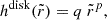
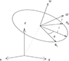 |
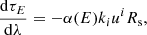
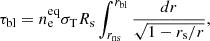
Fig. 2. Geometry for the Cartesian triad attached to a photon directional versor |


The geometry for deriving these components is shown in Fig. 2 and shall be used also for computing the Compton scattering.
We considered in the LF a reference system xyz where a photon has unit versor  . We also considered another direction,
  , which first we identified as the (normalized) electron velocity vector with which the photon interacts.
It is possible to define another orthonormal reference by mean of two additional unit vectors q1 and q2 which are mutually orthogonal between them and with  . Defining the versors components
  , the two other orthonormal versors are
  and
and  (Peplow 1999).
Defining the angles Θ and ϕ such that  , with ϕ increasing while going from q1 to q2, the vector
  can be written in a reference system xyz as
 (23)
(23)
For isotropic electron distribution in the fluid frame  , cosΘ ≡ μ, while ϕ is uniformly sampled over the interval [0 − 2π].
As Compton scattering is easier to be treated in the ERF once the electron velocity vector is defined, the photon space components klab in the LF tetrad are transformed to the ERF through the relativistic aberration equation (Pomraning 1973)
![Mathematical equation: $$ \begin{aligned} \mathbf k _{\rm erf}= \frac{1}{D} \left[(\mathbf k _{\rm lab}- \frac{\gamma }{\gamma + 1} (1 + D) ~ \mathbf{v}_{\rm el}\right], \end{aligned} $$](/articles/aa/full_html/2025/10/aa54222-25/aa54222-25-eq47.gif) (24)
(24)
where D = γ(1 − klab ⋅ vel) is the usual Doppler factor, with  . The reverse relation for getting klab from kerf is obtained from Equation (24) by replacing vel → −vel.
With reference to Fig. 2, we now identify  , and build the triad attached to the photon by aim of versors q1 and q2.
To compute electron scattering in the case of polarized radiation, one needs to know the space components of the electric field in the ERF. As for the photon momentum ki, we first derive f(i) components in the tetrad (LF) from fi using Eq. (17), and then apply the gauge condition so that f(t) → 0. We define ℰlab = (f(x), f(y), f(z)) as this three-dimensional space electric field vector. The space components of the magnetic field are thus obtained from Blab = klab × ℰlab. Subsquently, ℰlab and Blab are derived in the ERF with the Lorentz transformations
 (25a)
(25a)
 (25b)
(25b)
Defining  as the post-scattering photon direction, the scattering angle Θ between kerf and kerf′ and the azimuthal angle ϕ with respect to the electric field ℰerf are sampled following the procedure reported in Appendix A. The components of kerf′ are then obtained from Eq. (23).
The photon energy before scattering in the ERF is obtained with the usual Doppler formula
 (26)
(26)
After selecting the scattering angle Θ, we derived photon energy Eerf′ following Eq. (A.2).
Because each single photon is always polarized at 100%, one must use the post-scattering polarization degree for fully polarized radiation (Matt et al. 1996):
 (27)
(27)
After the scattering, we take into account the photon partial polarization for the next interaction drawing a new random number ξ testing a uniform probability distribution: if ξ < P, the new electric field vector is (Angel 1969)
 (28)
(28)
otherwise it is sampled randomly in the plane perpendicular to the new direction kerf′.
Then, we first derive Berf′=kerf′×ℰerf′ and back-transform to LF to obtain ℰlab′ and Blab′ inverting relations in Eqs. (25a) and (25b). The same is done to obtain klab′ using the inverse relation in Eq. (24). Now defining,  and
and  in the tetrad basis, we obtain components k′, i and f′, i in the coordinate basis using Eq. (17).
3.4. Output spectra and polarization
When a photon escapes from the system, we stop the integration at λ = 5 × 10³ rs, where the components of the metric tensor of Eqs. (2a)–(2e) differ from the flat-space case by less than 10−4.
We first convert the photon momentum components from the basis coordinate to spherical coordinates with the relation
 (29a)
(29a)
 (29b)
(29b)
 (29c)
(29c)
Subsequently, we convert from spherical to Cartesian components kx, ky and kz using the coordinate-dependent transformation matrix (Pomraning 1973).
To collect angle-dependent spectra and polarization parameters, the detector plane is seen as an imaginary sphere centered at the origin of the coordinate system, and divided into M belts equally spaced over μ = cos θ with Δμi = 1/M. For axisymmetric problems, photons collected in the lower hemisphere (θ > π/2) which have kz < 0 are assigned to the corresponding belt of the upper hemisphere by setting kz → −kz. The number of belts (i.e., angle-dependent spectra) needs a trade-off between the desired resolution and the statistics of the output spectra. The results presented in this work have been obtained with M = 10.
The polarization four-vector components at the detector collecting point are obtained by solving the linear system of three equations as explained in Sect. 3.1, and similarly then converted to Cartesian components.
For each collected photon, the Stokes parameters Q and U in given energy bin Ei − Ei + 1 and viewing angle interval μj − μj + 1 are calculated following Eqs. (15)–(19) in Matt et al. (1996). The total PD and PA are then obtained from
 (30a)
(30a)
 (30b)
(30b)
 (30c)
(30c)
 (30d)
(30d)
where N is the number of photons collected in the given bin of energy and viewing angle. Counting statistics error bars shown in plots are computed at 1σ level according to Elsner et al. (2012).
4. Setup of the bldisk model
4.1. Photons from the accretion disk
We consider a general wedge-like geometry for the disk, with an electron scattering atmosphere of constant height hphot = 0.2rs located above its surface governed by the law
 (31)
(31)
where  is the radial coordinate in the equatorial plane. Actually, the use of the cylindrical coordinate
 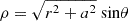 would be formally more correct in the above equation. However, it is straightforward to verify that given the value of a associated with the NS spin and that the inner disk is located at ∼3 Rg (see Fig. 1 and Sect. 4.4), the second term under the square root is less than 1% compared to the r-coordinate, and it becomes entirely negligible at larger radii. Consequently, to avoid unnecessary complications in the mathematical formalism presented below, we used
  , which under these conditions can be safely interpreted as a physical radius.
We note that for the non relativistic disk model of Shakura & Sunyaev (1973), p = 9/8. The deviation from a pure linear relation between height and radius with p = 1 is marginal in terms of global output, so in the rest of the work we consider this latter case.
The disk atmosphere is isothermal to the local BB temperature, and is characterized by an optical depth to electron scattering τdisk = neσThphot, which is a free parameter of the code.
The rest-frame photon emissivity law is derived from PT74 for a thin disk confined to the equatorial plane, with
 (32)
(32)
where  and F(x, a) is a function of the radial position and spin. The mass accretion rate is defined as
 (33)
(33)
where m is the mass of the compact object in units of solar masses, and ̇m is a free parameter of the simulations, the coefficient coming from the Eddington accretion rate.
The BB effective temperature at given radius  in the disk comoving frame is
 (34)
(34)
where σsb is the Stefan-Boltzmann constant.
To sample photons from the disk it is worth to remind the relativistic invariant (SK13)
 (35)
(35)
where fcol is the color-temperature correction factor,  is a normalized limb-darkening effect function,
  is the rest frame cosine of the emission angle with respect to the disk normal, dA is the proper area, and d
 the emission solid angle in the comoving frame.
The relativistic redshift factor ut is the time-component of the disk four-velocity ui, and for a pure azimuthal motion the condition uiui = 1 implies
 (36)
(36)
where gtt and gtϕ are defined at coordinates r and θ, while the disk Keplerian angular velocity is computed at the corresponding projected radius  and is
 (37)
(37)
The polar coordinate θ which appears in the metric tensor components of Eq. (36) is not equal to π/2 as for the simplest case of a disk located at z = 0, but is found by numerically solving equation
 (38)
(38)
where  , with the first term given in Eq. (31).
Assuming that flimb and fcol do not depend on radius, the photon rate from a disk elementary proper area as measured by a distant observer is
![Mathematical equation: $$ \begin{aligned} \mathrm{d}\dot{N}^\mathrm{disk}(r) = \frac{[T^\mathrm{eff}_{\rm bb}(\tilde{r})]^3 }{f_{\rm col}u^{t}}~\mathrm{d}A, \end{aligned} $$](/articles/aa/full_html/2025/10/aa54222-25/aa54222-25-eq83.gif) (39)
(39)
where dA can be computed from the determinant of the induced metric tensor on the disk surface multiplied by the Lorentz gamma factor (Poisson 2004; Wilkins & Fabian 2012):
![Mathematical equation: $$ \begin{aligned} \mathrm{d}A = \gamma \left[g_{rr}~g_{\phi \phi }+ g_{\theta \theta }g_{\phi \phi }\left(\frac{\mathrm{d}\theta }{\mathrm{d}r}\right)^2\right]^{1/2}\mathrm{d}r~\mathrm{d}\phi , \end{aligned} $$](/articles/aa/full_html/2025/10/aa54222-25/aa54222-25-eq84.gif) (40)
(40)
where
 (41)
(41)
with  .
.
The relativistic Doppler factor γ = (1 − β2(ϕ))−1/2, which corrects for the disk orbital motion, can be computed from the azimuthal component of the velocity as seen from the locally non-rotating frame (Bardeen et al. 1972):
 (42)
(42)
where uϕ = utΩk.
For axisymmetric problems, the function  as well as the photon rate do not depend on the azimuthal coordinate ϕ, while they do for more complicated configurations such as a tilted or warped disk (Hartnoll & Blackman 2000; White et al. 2019).
The total number of photons emitted by the whole disk per observer unit time is
 (43)
(43)
For the case p = 1, the integration boundaries in Eq. (43) are
 (44a)
(44a)
 (44b)
(44b)
where θd ≈ arctan(1/q), while  and
and  are the inner and outer disk radius on the equatorial plane. The fraction of photons emitted between rmin and a generic radius r is then
![Mathematical equation: $$ \begin{aligned} \xi (r) = \frac{1}{\dot{N}_{\rm tot}^\mathrm{disk}} \int ^{2\pi }_{0} \int ^r_{r_{\rm min}} \frac{[T_{\rm eff}(\tilde{r}\prime )]^3 }{u^{t}}\mathrm{d}A\prime . \end{aligned} $$](/articles/aa/full_html/2025/10/aa54222-25/aa54222-25-eq94.gif) (45)
(45)
Once defined the disk parameters  and p, a pre-tabulated grid of values ri − ξi is preliminarly computed at the beginning of the run using Eq. (45), with r0 = rmin, rN − 1 = rmax, ξ0 = 0 and ξN − 1 = 1.
At computation time, for any newly generated photon a random number is drawn from the uniform distribution between 0 and 1, and the corresponding radius of photon emission r is computed by linear interpolation. The BB effective temperature is then computed with aim of Eqs. (32) and (34) at the corresponding position in the equatorial plane  , and subsequently we sample a photon energy from a Plank distribution with Tbbcol = fcolTbbeff following the procedure described in Appendix B.
 |
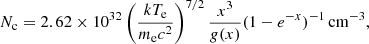
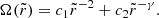
Fig. 3. Polarization degree as a function of viewing angle for emerging radiation with seed photons located at the base of a slab with different optical depths. The results were obtained using the iterative method described in F24. Positive and negative values correspond to a PA coplanar with the slab or perpendicular to it, respectively. |
We simulate photons at the top of the disk atmosphere with initial angular distribution  and PD
 depending on the value of τdisk. The distributions are pre-computed using the iterative scattering method described in F24 (see Fig. 3). In this way, the disk normalization (i.e., total number of photons) is the same for any value of τdisk, but its flux at different observer viewing angle depends not only on light bending effects due to space-time curvature, but also on τdisk.
For sampling photons in the disk local fluid frame, we adopt the tetrad formalism defined in S11. In this basis the photon momentum components in the upper hemisphere are
 (46a)
(46a)
 (46b)
(46b)
 (46c)
(46c)
 (46d)
(46d)
where  is the direction with respect to the disk surface normal in the fluid frame, while
  is drawn uniformly over the interval [0 − 2π]. Here and below we use the notation
  and
and  to avoid confusion with the angular coordinates θ and ϕ defining the metric tensor. Once sampled the photon momentum direction in the tetrad, we obtain its components ku in the coordinate basis with the conversion matrix in Eq. (17) and then start to follow its path. It may happen that photons reach the top of the disk atmosphere. In this case, the latter acts both as a reflector and a polarizer with an efficiency in both processes depending on τdisk. However, if an external photon manages to pass through the atmosphere and reaches its base, it is considered as absorbed.
4.2. Seed photons from NS surface
The procedure for generating BB seed photons from the NS surface is similar to that for the accretion disk, with slightmodifications related to the geometry. In particular, we consider a sub case of Eqs. (A1)–(A13) of S11, where h′(r) = cos θ, ur = 0, and Ω = Ωns for defining the tetrad.
The angular distribution of photons is determined with respect to the normal of the NS surface, which is now identified by the  coordinate of the space tetrad. Photon momentum space components are thus defined as
 (47a)
(47a)
 (47b)
(47b)
 (47c)
(47c)
 (47d)
(47d)
Photons are simulated assuming an isotropic and unpolarized distribution at the top of the NS photosphere; thus  and
and  are sampled uniformly over the intervals [0 : 2ϕ] and [ − 1 : 1], respectively.
The total photon rate from the NS surface is
 (48)
(48)
where γ can be obtained from Eqs. (36) and (42) by replacing Ωk with Ωns as the NS angular velocity measured by a distant observer.
The integration over the polar angle in Eq. (48) is computed up to θmin = π/2 − θns, where θns is the maximum latitude above the NS equator from which photons are generated. We consider the region above θns as a dark zone where the emissivity, if present, does not contribute in the X-ray band (Inogamov & Sunyaev 1999, hereafter IS99), and which also plays as full absorber for the photons impinging on it. A similar modeling with varying latitude of the emitting region around the NS has also been adopted by B25, who considered a simple BB spectrum to investigate energy-dependent relativistic effects on polarized radiation.
The components of the metric tensor in Eq. (48) are defined at fixed radial coordinate r = rns, while the gravitational redshift factor ut is defined as in Eq. (36) by substituting Ωk with Ωns. We assume a NS radius rns = 2.42rs, corresponding to 10 km for a NS mass of 1.4 M⊙.
Each photon on the NS surface is generated with azimuthal angle ϕ uniformly sampled between 0 and 2π, then another random number ξ is drawn and the polar angle θ is obtained by the inverse relation
 (49)
(49)
To speed up computation, also in this case a grid of pairs ξi − θi is precompiled at the beginning of the simulation, and the polar angle θ is obtained by linear interpolation for given random number ξ.
If a photon in its random walk across the BL (see Section 4.3) is back reflected to the NS zone below the BL itself, we treat it as it follows: we consider scattering off electrons at the NS temperature Tbb and if after the scattering the radial component of the photon momentum is positive (i.e., outward) then we newly start to track it, otherwise we consider it as absorbed. For typical temperatures of the NS photosphere and BL, both of which are of the order of a few keV or less, the electron scattering cross-section follows within a few percent the Thomson regime with an angular dependence dσ ∝ (1 + cos2Θ). This symmetric backward-forward behavior implies a NS albedo of A ∼ 0.5, with half of the returning photons being absorbed and the other half being reflected.
It is finally worth highlighting that the total photon rates derived in Eqs. (43) and (48) for the disk and NS respectively are computed in the upper hemisphere with θ < π/2. To simulate photons above and below the midplane, in both cases when a photon is generated, we further draw a random number ξ: if ξ < 0.5 the photon starts its travel from the upper hemisphere, in the other from the lower hemisphere.
4.3. Geometry of the boundary layer
Following part of the geometrical and thermodynamical results of IS99, we consider a BL at constant temperature kTe extending up to a latitude θbl which is a free parameter of the simulations and which is equal to θns, providing a covering factor equal to one. This choice is also observationally motivated by the fact that in the framework of the EM, usually the direct BB component at ∼1–2 keV attributed to the NS is not observed, a part from the particular case of the NB of GX 5-1 (Fabiani et al. 2024). Actually, unscattered BB radiation can be seen either if there is no medium obstructing the line of sight, with θns ≳ θbl, or if the seed photons have an almost uniform distribution over the Comptonization zone (Titarchuk et al. 1997).
To mimic a BL which is radially slightly more extended in the equatorial plane with respect to higher latitudes (see Fig. 1 of IS99), we defined an analytical function
 (50)
(50)
with
 (51)
(51)
where k = 0.85 and rbl = 1.2rns. While both numerical coefficients contain a certain degree of arbitrariness, it is equally true that they are qualitatively of the order given in IS99. The limited latitudinal extent of the BL latitude breaks the spherical symmetry and the polarization of the Comptonized BB spectrum is not zero, yet remaining relatively low (see Sect. 2).
To define the electron density given the optical depth τbl we consider the space line element
 (52)
(52)
where α, β = 1, 2, 3 (Landau & Lifshitz 1975). For a rotating compact object, the terms of the metric tensor g03 are non-zero, and the expression contains a dependence on θ even for the case dθ = 0 and dϕ = 0. However, for r ≳ rns and a ≲ 0.2 the deviations from the non-rotating case are marginal and it is possible to simplify the expression in Eq. (52) using the Schwarzschild metric. We then define the electron density from the relation
 (53)
(53)
where Rs is the NS Schwarzschild radius and σT the Thomson cross-section. The integral function in Eq. (53) has analytical solution in the form
![Mathematical equation: $$ \begin{aligned} F(r) = r \sqrt{1- \frac{r_{\rm s}}{r}} + r_{\rm s}\mathrm{arctanh} \left[\sqrt{1-\frac{r_{\rm s}}{r}}\right], \end{aligned} $$](/articles/aa/full_html/2025/10/aa54222-25/aa54222-25-eq120.gif) (54)
(54)
so that eventually one obtains from Eqs. (50) and (53)
![Mathematical equation: $$ \begin{aligned} n_{\rm e}(\theta ) = \frac{\tau _{\rm bl}}{\sigma _{\rm T}R_{\rm s}\{F[W(\theta )]-F(r_{\rm ns})]\}}\cdot \end{aligned} $$](/articles/aa/full_html/2025/10/aa54222-25/aa54222-25-eq121.gif) (55)
(55)
A quasi-constant radial optical as a function of the latitude is not far from what is reported in Figs. 9 and 10 of IS99. We also note that we do not model the sharp increase of the surface density Σs (i.e., the optical depth) close to the equatorial plane, but this occurs is a small region which is intercepted by the disk in touch with the BL, so that it essentially does not contribute to the observed hard radiation spectral formation. Moreover, as shown by IS99, the BL emissivity itself may have a latitudinal dependence, achieving its maximum close to θbl, but in the context of a MC modelization, this would require a definition of a BB temperature depending on θ as well. We believe that this is an unnecessary complication, considering that the information contained in the data does not allow this trend to be described at such a detailed level.
Concerning the BL matter velocity, we neglect the radial and polar components, the latter related to its spreading to latitudes above the equatorial plane, and consider uϕ = utΩbl with sub-Keplerian angular velocity profile given by
 (56)
(56)
The constants c1 and c2 as well as the Reynolds number γ are obtained by imposing the boundary conditions in the equatorial plane Ωbl(rns) = Ωns and Ωbl(rbl) = Ωk(rbl), together with the continuity condition for the derivative Ωbl′(rbl) = Ωk′(rbl) (Titarchuk & Osherovich 1999).
4.4. Construction of the table model
To create the grid of the bldisk model we proceeded in the following way. First we selected the free parameters of the simulation, and for each of them we defined the boundaries as well as the number of point in the grid (see Table 1). Concerning the parameters kept the same in each run, we selected a NS spin νns = 500 Hz, corresponding to a value a = 0.117 in the metric tensor, and have checked that differences with the case of a non-spinning NS are negligible. The inner disk radius has been set equal to the equatorial BL radius, with rbl = rin and rbl = 1.2 rns, while the outer radius has been fixed to rmax = 1000 rs. The local BB spectrum of the accretion disk at any radius is corrected by a spectral hardening factor fcol = 1.7 (Shimura & Takahara 1995), similarly to what has been done for the diskpn model (Gierliński et al. 1999).
List of parameters used to create the grid of the bldisk model.
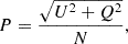
 |
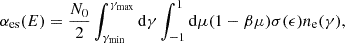
Fig. 4. Example of spectra obtained from the bldisk model, with each free parameter varied in turn. Aside from the individual panels where they are varied, fixed parameters are: θbl = 50°, kTbb = 2 keV, kTe = 3 keV, τbl = 4, ṁ = 1, τdisk = 5, |

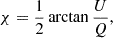
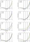 |
Fig. 5. Polarization degree as a function of energy derived from bldisk using the same parameter combination as that reported in Fig. 4. For axisymmetric geometries PD =|Q|, so angle rotation with PA switching from orthogonal (Q > 0) to parallel (Q < 0) direction to the symmetry axis occurs at the energy where PD =0. The vertical lines represent the IXPE energy bands 2–4 keV and 4–8 keV, respectively. |
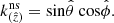
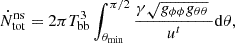
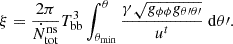
As it can be seen from Table 1, a total of 1.6 × 10⁴ runs has been performed, and for each of them the triplets (I, Q, U) for ten intervals of observer viewing angle are computed, leaving a total of 4.8 × 10⁵ Stokes spectra to be stored in the grid. We note that because of the azimuthal symmetry of the problem, actually all the U spectra are zero.
The photon spectra have been computed in the energy range 0.1–70 keV, while for the Q spectra we have considered the 0.1–20 keV bandpass. Runs have been performed on the computing cluster of INAF-Bologna, equipped with 96 logical cores per node. For each simulation 1.25 × 10⁶ photons/core have been generated, for a total of 1.2 × 10⁸ photons for simulation. To smooth out the statistical fluctuations of each spectrum, we applied a Savitzky-Golay filter with a specifically dedicated Python suite in the post processing phase, before storage in the FITS table.
In order to pass to physical units, we consider that the flux collected by all the observers located along the direction μ in a polar-angle interval Δμ is
 (57)
(57)
where L(μ) is the source photon or energy angle-dependent luminosity and the factor 2π in the denominator comes from integration over the azimuthal angle. All spectra have been multiplied by a constant obeying the relation
 (58)
(58)
where F(μ)sym is the angle-dependent simulated flux (depending on the number of generated photons), ϵ ≤ 1 is the fraction of collected over simulated photons, η(μ) < 1 is the percentage of photons over the direction μ,  is the total photon luminosity in physical units, and D10 is the source distance computed at 10 kpc. The bolometric photon luminosity in physical units is obtained multiplying Eqs. (43) and (48) by 2.37 × 1032Rs2, where the coefficient is the Stefan-Boltzmann constant for BB photon spectrum with temperature measued in keV and Rs is the Schwarzschild radius for given compact object mass. Then, the bldisk normalization parameter at the XSPEC prompt is proportional to 1/D102 and provides an independent estimate of the source distance.
The final writing to FITS table with format required by the XSPEC package has been done with the HEASP Python module, which manipulates files associated with high energy astrophysics spectroscopic analysis2.
5. Results
5.1. Spectropolarimetric layout
Before discussing the application of bldisk to observational data, we shown in Fig. 4 a series of theoretical spectra in EF(E) units obtained by varying each time the value of one of the free parameters. This may give an idea about the contribution of each physical or geometrical quantity to the total spectrum.
For each group of spectra with varying parameters, in Fig. 5 we show the corresponding PD value as a function of energy. For statistical reasons related to the number of photons in the simulations, the results are shown up to 20 keV. Of course, there can be numerous multiparametric combinations; therefore, we limited our analysis to a few representative cases.
In the PD figures, we also indicate the energy band of IXPE to highlight the interval in which the model can be tested against observations. It can be seen that the plots display two distinct regions above and below a energy-depedent turning point, corresponding to the parts dominated by the disk and by the combination of Comptonization and reflection, respectively. Indeed, except for the case in which it is varied, all results are shown with τdisk = 5, for which the disk PA is perpendicular to the system axis (see Fig. 3). An aspect worth considering, and one that is generally overlooked, is the fact that just as the disk acts as a reflector and polarizer for the Comptonized radiation coming from the BL, the latter can also reflect and polarize the radiation coming from the disk. One can therefore speak of BL-reflection as an additional component to the spectropolarimetric signal.
We provide a brief explanation of the spectropolarimetric layouts for each parameter of bldisk below:
-
θbl (Figs. 4a and 5a): an increase in the BL latitude leads to a higher normalization of the high-energy part of the spectrum, which also becomes harder. This can be readily explained by considering that NS seed photons diffuse through the BL in both radial and latitudinal directions. Thus, if θbl increases, the optical depth along the meridional direction also increases, causing photons to undergo a greater average number of scatterings k before escaping, and thereby emerging with a higher mean energy according to (Rybicki & Lightman 1986):
 (59)
(59)A progressive increase in the BL latitude results in a larger fraction of both Comptonized as well as disk-reflected flux. Since these two components are polarized perpendicularly to that of the direct disk emission, the energy at which the PA rotation occurs gradually shifts to lower values.
-
kTbb (Figs. 4b and 5b): the spectropolarimetric layout as a function of the NS photospheric BB temperature is qualitatively similar to the case of varying BL latitude. In this case, an increase in kTbb results in a higher number of seed photons, which impacts the magnitude of the high-energy part of the spectrum, which gets harder due to the higher average energy of the initial photons (see Eq. (59)). Again, as kTbb increases, a greater number of Comptonized photons impinge on the disk atmosphere, enhancing both the reflected component and the associated polarization.
-
kTe (Figs. 4c and 5c): when the electron temperature of the BL is varied, its effects are evident in terms of spectral hardening, while they are negligible for what it concerns the observed PD in the IXPE band. It is interesting the behavior of the PD above 10 keV, which appears as the combined effect of reflection from both the disk and the BL. In fact, as the temperature increases, the polarization degree of the scattered radiation decreases; therefore, for the same number of photons coming from the disk, a cooler BL is a more effective polarizer than a hotter one (Matt et al. 1996; McNamara et al. 2009). Its effect also appears to be dominant, since intuitively one would expect that a harder Comptonized primary spectrum would produce a higher disk-reflected polarized signal.
-
τbl (Figs. 4d and 5d): for a given kTe, a higher optical depth gives a harder spectrum, reflecting a higher value of the Compton parameter (Rybicki & Lightman 1986; Sunyaev & Titarchuk 1980). At the same time, it is important to note that the albedo at the NS surface is A ≈ 0.5, due to the quasi-Thomson cross-section when Compton scattering occurs at the base of the NS atmosphere (see Sect. 4.2). For radiation originating at the base of a scattering medium, the number of photons back-reflected increases as it becomes progressively more opaque (see Fig. 8 in F24). Since the number of photons impinging on the disk increases as τbl decreases under conditions of albedo A < 1, the PA swap occurs earlier. As a consequence, the rising phase after the turning point also starts earlier, and disk reflection becomes more effective. However, as in the case of the dependence on kTe, the differences in the PD magnitude are likely not large enough to be detectable by IXPE. A detailed treatment of the NS photosphere albedo is beyond the scope of this work, so the implicitly derived value of A is considered a reasonable compromise between a full absorbing and perfectly reflecting NS photosphere.
-
ṁ (Figs. 4e and 5e): the mass accretion rate of the disk also plays a key role in shaping both the photon spectra and the polarization properties. Spectroscopically, it determines not only the total flux in the energy range where the disk dominates but also the magnitude and position of the spectral rollover energy, combined with the contribution from the BL Comptonization spectrum. The PD in the IXPE band strengthens as ṁ decreases, as a result of the drop of the disk flux and the consequent weakening of the mutual cancellation effect between the two orthogonal PAs between the disk itself and the Comptonization plus reflection components.
-
τdisk (Figs. 4f and 5f): for given values of ṁ and
 , we set the condition that the total number of disk photons is the same for any value of τdisk. If the number of disk photons remains unchanged, the rest-frame angular distribution of the specific intensity
  does not, as it is dictated by the optical depth of the atmosphere. It is important to outline this point because τdisk, similar to the other bldisk parameters, not only plays a crucial role in the polarimetric signal, but also concurs in determining the disk flux observed as a function of the viewing angle, which would be not the case for disk rest-frame isotropic emissivity (out of gravitational light bending effects).
For τdisk ≲ 3, there is no angle swap, with disk PA aligned with the system spin axis; this can be seen directly in Fig. 3 where for low values of τ, Q < 0 for a broad range of angles with respect to the normal of the slab. We outline this crucial point: together with PD, also PA rotation with energy is a quantity that IXPE can detect and thus work as powerful diagnostic for any theoretical model. It is also interesting to note the PD behavior for τdisk = 0; in this case indeed the disk is treated as a full absorber, and reflection from it is not present. The PD observed to increase up to 3% at 20 keV cannot be the direct component from the BL, as this value is well above the maximum limits established by F24 and B25. The only remaining possibility is that this polarization arises from single or at least double scattering of disk photons that externally illuminate the BL.
-
 (Figs. 4g and 5g): the disk aspect ratio, usually not considered in disk models where the emission is assumed to occur in the plane z = 0, is an additional parameter that contributes to shaping the spectropolarimetric layout. For a fixed outer radius
  , progressively increasing values of
  very marginally affect the total number of disk photons, resulting in no net impact on the spectral output for the chosenparameter combination, so we show spectra multiplied by a scaling factor. However, a higher aspect ratio increases the solid angle subtended by the disk as seen from the BL. As a consequence, reflection becomes stronger, enhancing the observed PD at E ≳ 2 keV. It is also worth noting how
  influences the PD at lower energies: indeed, as it increases, for a given source inclination iobs, the average angle between the direction of photons reaching the observer and the disk normal in the fluid frame decreases, leading to a lower measured polarization. These combined effects, in turn, play a role in shifting the energy at which the PA swap occurs, along with an inverse PD magnitude dependence on
  above and below that threshold.
 -
iobs (Figs. 4h and 5h): finally, we consider the effects of the source viewing angle. For a disk with Chandrasekhar-like polarization, the angular distribution of the rest-frame specific intensity is such that the flux is higher for face-on configurations than for edge-on ones (ST85). This also translates, from the observer’s point of view, into a reduced contribution from the disk. The same angular dependence applies to the BL configuration, except in the case of full coverage of the NS surface. In fact, for a fixed BL maximum latitude, the photon flux observed at high inclination angles iobs is greater than that observed along the direction progressively aligned with the system axis. This primarily results in a change in the normalization of the Comptonized component, while its spectral shape remains essentially unaffected. The interplay between the disk and BL components also leads to a shift in the peak energy of the EF(E) spectrum as a function of the viewing angle. Not surprisingly, the PD has a strong dependence on the system inclination; in particular, for highly inclined system, the PA swap fully occurs in the IXPE band and can be detected. It is interesting to note that the higher the energy at which the PA swap occurs, the shallower the PD gradient as a function of energy within the IXPE band.
5.2. Model application to observed spectra
Following the same approach adopted for other XSPEC models such as comptb (Farinelli et al. 2008) or compmag (Farinelli et al. 2016), we tested bldisk using previously performed spectropolatimetric X-ray observations. What is new here with respect to previous models, is the possibility to fit simultaneously not only the “standard” photon spectra, but also the (Q, U) spectra provided by IXPE. As the Stokes parameters (Q, U) of the model are defined in a reference frame where the vertical axis is aligned to the projection of the system spin axis in the sky, in the fitting procedure it is necessary to define a new free parameter, the roll angle ψ, which corrects for the unknown rotation of the detector plane with respect to the source symmetry axis (the latter not to be confused with the inclination angle), and rotates the (Q, U) Stokes values accordingly. This additional rotation component is defined in XSPEC by the polrot multiplicative model.
To correct for calibration issues in the IXPE response matrix, we also applied the gain model command, which shifts the energies on which the response matrix is defined and the effective area curve to match. The parameters for the (Q, U) spectra were linked to those of the I-spectra. Finally, a systematic error of 0.5% was added to all spectra.
In the present work we selected two bright test sources, Cyg X-2 and GX 9+9, representative of the Z and atoll class, respectively. Data are taken from the recent multi-instrument observational campaigns performed by IXPE along with other X-ray facilities.
5.3. Cyg X-2
Cyg X-2 is one of the most studied Z sources (e.g., Di Salvo et al. 2000; Titarchuk et al. 2007; Farinelli et al. 2009; Ludlam et al. 2022) and a spectropolarimetric observational campaign was carried on by F23 with IXPE, NICER and INTEGRAL data. The authors fitted the broad-band spectrum with a multicolor disk BB (diskbb; Mitsuda et al. 1984) plus the Comptonization model comptt (Titarchuk 1994) and a Fe emission line, and found a PD =1.85 ± 0.85% in the 2–8 keV. The model-independent analysis showed a PD increasing with energy between 2–4 keV and 4–8 keV and no PA rotation, while from the spectropolarimetric fit, some evidence of orthogonality was found for the PA between the disk and Comptonization component. Even when fixing  , only an upper limit of ≲3% could be placed for the disk PD, while for the hard component the authors found a PD ∼4 ± 2%. As outlined by F23, the latter value very likely encompasses a relevant contribution from the reflection, which must be present but could not be efficiently detected by the JEM-X instrument due to its low energy resolution. One of the most important results was the discovery that the PA of the source was aligned to that provided by former radio jet observations, allowing for much tighter constraints on the accretion geometry and the expected PA behavior. To date, such an absolute measurement of the PA in a bright NS-LMXB has been available only for Cyg X-2 and Sco X-1 (Long et al. 2022; La Monaca et al. 2024a).
Here, instead of the joint NICER and INTEGRAL spectrum, we analyzed NuSTAR data collected on May 5 2022 for about 39 ksec (Obs. ID 30801012002) as NuSTAR provides better energy resolution and higher statistics in the energy range 3–40 keV, with respect to the INTEGRAL data. We did not include the NICER data because of several calibration issues (e.g., the need of adding artificial absorption edges in its spectra), and mainly because during both NICER observations the source moved across the NB of the color-color diagram with time-scales of hours to minutes typical of Z sources (see Fig. 3 in F23). The NuSTAR observation partially overlap only to the second NICER observations, posing some problems in fitting the joint spectra due to possible spectral evolution at lower energies ≲3 keV. Instead, we used the IXPE I-spectra to provide spectral coverage down to 2 keV, with the addition of the (Q, U) spectra which are fitted correspondingly by their counterpart in the bldisk FITS table.
The model we used to fit the broad-band spectrum is const*tbabs*edge*polrot*(bldisk+polconst*gauss) with fixed PD = 0 in polconst for the emission line. The photo-electric absorption was modeled with the tbabs multiplicative component (Wilms et al. 2000). The residuals of the NuSTAR spectra show some evidence of an absorption feature around 9 keV, related to the iron line absorption edge.
The first natural attempt was to perform the fit with all bldisk parameters left free: this provided a very good χ2/d.o.f. = 1543/1438 and no systematic residuals across the 2–40 keV energy band, yielding a very comfortable result about the goodness of the model in catching source spectral properties. More specifically, we found θbl = 90° (> 76° ), kTbb = 1.52 ± 0.04 keV, kTe = 3.7 ± 0.2 keV, τbl = 4.6 ± 0.3, ṁ = 0.2 ± 0.03, τdisk = 3.2 ± 0.8, iobs = 42 ± 3°,  , and a normalization Nbldisk = 2.1 ± 0.3.
While these parameters are entirely reasonable and consistent with those typically found for the HSS of bright NS-LMXBs, the derived value of τdisk at an inclination of approximately 40° would correspond to a disk PA aligned with the system axis, as suggested by the negative value of Q shown in Fig. 3. This appears to be in tension with the findings of F23, where spectropolarimetric analysis pointed toward an orthogonality between the disk PA and that associated with the BL and reflection components, which are instead roughly aligned with the system axis. The model is therefore statistically acceptable, though it shows a mild discrepancy when compared to earlier findings in terms of polarimetry.
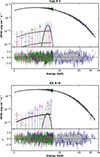 |
Fig. 6. Deconvolved EF(E) spectra of IXPE (I, Q, U) and NuSTAR of Cyg X-2 (upper panel) and GX 9+9 (lower panel) with the best-fit model reported in Table 2 superposed and residuals between data and the model in units of σ. The greater rolling angle of Cyg X-2 makes visible the U component of the bldisk spectrum in the IXPE detector reference frame. |
Best-fit spectral parameters of the model applied to the IXPE (I, Q, U) and NuSTAR spectra of Cyg X-2 and GX 9+9.
To be more consistent with the results of F23, we performed a fit with fixed τdisk = 5. This yielded a statistically equivalent result (see Fig. 6), and on the basis of the above considerations we consider this model as preferable, with its best-fit parameters reported in Table 2. We note that if from one side the best-fit value of the BL latitude would correspond to a total NS coverage, the parameters are less constrained than the others, with a lower boundary consistent with a moderate latitudinal extent of 45°.
The statistics of the (Q, U) IXPE spectra on the other hand contributes marginally to the total χ2, so instead of looking at the (Q, U) residuals between data and model, we show in Fig. 7 the PD behavior as a function of energy derived from the bldisk best-fit parameters overplotted on the PD error boxes at 3σ confidence level in the 2–4 keV and 4–8 keV, as reported in F23 and obtained with PCUBE (Baldini et al. 2022). The plot shows a linear increase of the PD starting already at ∼0.4 keV, driven by the value of ṁ, with a PA swap occurring well below the IXPE band – see Fig. 5 for the case of varying the latter parameter. The model-predicted values intersect the IXPE error boxes in both the 2–4 keV and 4–8 keV bands. We also extrapolated the PD trend up to 20 keV, observing a continued rise reaching up to more than 6%. Most likely, this monotonic increase is driven by disk reflection, since at energies ≳8 keV the direct disk contribution becomes progressively negligible, while the BL, in the proposed configuration, does not exceed a PD ∼1% (F24, B25).
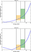 |
Fig. 7. Polarization degree as a function of energy for Cyg X-2 (upper panel) and GX 9+9 (lower panel) as obtained from the best-fit parameters of Table 2. The two boxes represent the PD boundaries at 3σ confidence level in the 2–4 keV and 4–8 keV energy bands, as measured with the PCUBE algorithm. |
5.4. GX 9+9
The bright atoll GX 9+9 is characterized by having a rather stable soft state spectrum (Gladstone et al. 2007), and a modulation of 4.2 h has been observed in both the optical and X-ray band (Hertz & Wood 1988; Schaefer 1990). A broad-band spectral study with joint XMM-Newton and BeppoSAX observations performed by Iaria et al. (2020) revealed the presence of a significant relativistic reflection component. The authors estimated and inclination angle of  deg and
  deg by modeling the spectrum in the framework of the EM and WM, respectively. It is interesting to note that Savolainen et al. (2009), using RXTE and INTEGRAL data, modeled the source spectrum by considering a geometry resembling that of Fig. 1, with an accretion disk and a SL around the NS, finding that the extent of the SL increased with luminosity and estimating a source distance of 10 kpc.
For testing the bldisk model, we used the NuSTAR and IXPE spectra of the joint observational campaign carried out on 2022 by U23. The authors fitted both the NuSTAR-alone and IXPE + NuSTAR spectra with a continuum model consisting of diskbb plus comptb, along with a reflection component which self-consistently encompasses Fe fluorescence line emission and in which the disk is illuminated by a BB spectrum assuming a radiation incident at 45° (relxillns; García et al. 2022). The source inclination angle as derived from relxillns was found to be iobs = 28 ± 8°, a value lower than those obtained by Iaria et al. (2020).
Concerning polarimetric results, in the 2–8 keV energy band U23 found a PD = 1.4 ± 0.3%, with some evidence of a trend of PD increasing with energy when comparing the 2–4 keV and 4–8 keV energy intervals. As for Cyg X-2, from the model-independent analysis of PCUBE the PAs in 2–4 keV and 4–8 keV ranges resulted to be aligned. However, from the model-dependent analysis with fixed PD = 1% for the Comptonization feature and the disk and leaving free the reflection component (with PArefl= PAcomp), the PA of the disk provided evidence of orthogonal alignment with respect to that of the other two components.
We tested for GX 9+9 the same model applied to Cyg X-2 initially allowing all parameters of bldisk to vary freely. This yielded a fully satisfactory fit, with χ2/d.o.f. = 1387/1480 (see Fig. 6). In this case, the fit returned a value of τdisk close to the upper bound of the model grid, associated with Chandrasekhar-like disk polarization. This result is consistent with the indication of orthogonality between the PA of the disk and that arising from the BL and reflection, as reported by U23. The best-fit parameters are listed in Table 2. The resulting PD as a function of energy fully overlaps with the IXPE error bars in both the 2–4 keV and 4–8 keV bands. Above the IXPE band, the extrapolated PA has a behavior qualitatively similar to that of Cyg X-2 (see Fig. 7), while PA rotation is expected below 1 keV, again out of the IXPE band, consistent with the observational result reported by U23 of a constant PA across the two energy intervals.
6. Discussion
In the previous sections, we presented the application to the spectropolarimetric analysis of a new tabular model for the XSPEC package (bldisk) specifically developed for bright NS-LMXBs in their HSS. The model is built as a FITS table obtained from MC simulations with a full general relativity treatment, and it allows for a simultaneous fit of the (I, Q, U) Stokes spectra of X-ray sources. The geometry we have considered is the one typical of the EM (see Fig. 1), toward which observational evidence–both temporal and polarimetric–seem to converge with respect to the WM, allowing for the disentangling that was not possible with simple spectroscopy (Done et al. 2007; Revnivtsev & Gilfanov 2006; Revnivtsev et al. 2013). Indeed, an extended optically thick corona illuminated from the bottom by the disk photons would give rise to a PA perpendicular to the system axis in the 2–8 keV energy band (ST85, F24), while a parallel PA is obtained for coronal low optical depths (Schnittman & Krolik 2010), which is not the case for the class of sources here considered.
While so far, thanks to radio imaging, an absolute measurement of the PA position has been possible only for Cyg X-2 and Sco X-1, it is equally true that, apart the case of 4U 1820-303 (Di Marco et al. 2023), a constant PA in the IXPE band has been observed in Cyg X-2 (F23), GX 9+9 (U23), 4U 1624–49 (Saade et al. 2024; Gnarini et al. 2024a), GX 13+1 (Bobrikova et al. 2024), XTE J1701−462 (Cocchi et al. 2023), and GX 349+2 (Kashyap et al. 2025), while due to very low PD it was not possible to place serious constraints about GX 3+1 (Gnarini et al. 2024b) and GS 1826–238 (Capitanio et al. 2023). This empirical similarity between the sources clearly suggests, by deduction, an almost common geometric configuration, further supporting the Eastern Model scenario.
We tested the bldisk model on the IXPE and NuSTAR spectra of two representative bright NS-LMXBs, namely the Z source Cyg X-2 and the bright atoll GX 9+9 for which IXPE provided polarimetric observations during observational campaigns joined with other X-ray observatories. To our knowledge, this is the first attempt of developing a physical model self-consistently computing the emission from the accretion disk, the Comptonization spectrum of the BL as well as reflection on the top of the disk by the BL photons, plus a fraction of direct disk photons which play as an external source of seed photons for the BL itself.
The reflection component, which may play a crucial role not only in the spectral formation but also, when not mainly, in driving the polarimetric signal, is computed by considering a scattering atmosphere above the disk surface. The optical depth of the atmosphere, labeled as τdisk, is a free parameter of the bldisk model and concurs in the spectropolarimetric layout in a two-fold manner. Firstly, the rest-frame angular distribution of the emerging photons depends on τdisk and the relation between observed disk brightness and inclination angle is monotonic for τdisk ≳ 2, with face-on inclinations having higher flux than edge-on. For lower optical depths instead, the behavior is more complicated, with the peak of emission achieved at inclination angles iobs ≲ 60° (ST85, F24). Secondly, the value of τdisk contributes to the determination of the net polarimetric signal with a magnification or a drop depending if the disk PA is aligned or orthogonal to that of the BL plus reflection components, with the latter parallel to the system symmetry axis (see Fig. 5).
We note that defining a scattering atmosphere above the disk might suggest a two-phase model with an accretion disk corona (ADC). In fact, in ADC models a fraction of the disk power is dissipated in the overlying corona, which can reach higher temperatures than the underlying disk in both NS and BH systems (Haardt & Maraschi 1991; Poutanen & Svensson 1996; Schnittman & Krolik 2010; Zhang et al. 2025). In our geometrical setup, the ADC is instead treated as the upper layer of the disk itself and acts as a polarizer for both the photons emitted from the underlying surface and the external Comptonized radiation emerging from the BL and impinging on the disk surface.
A fraction of reflected photons may originate from the disk itself as returning radiation (SK13), but unlike the case of BH sources, this effect is probably small due to the presence of the NS/BL, which have a vertical height scale of ∼3Rs and, contrary to BHs, may intercept a larger fraction of photons, especially in the inner region where curvature effects are stronger.
The electron temperature of the disk atmosphere is assumed to be isothermal and equal to the BB temperature at each radius, as determined by the Page-Thorne disk profile, similarly to the approach used by T21. However, those authors implemented a more detailed physical treatment using the CLOUDY code (Ferland et al. 2017) to determine the ionization properties of the atmosphere, and subsequently used the CLOUDY outputs to compute polarimetric predictions with STOKES (Goosmann & Gaskell 2007; Marin et al. 2012).
Once the primary external photon spectrum is defined, the amount and shape of the reflection component depend on the physical properties of the disk upper layers (George & Fabian 1991; Magdziarz & Zdziarski 1995; Nandra et al. 2007; García et al. 2013, 2022). In the case of partially ionized disks, bound-bound or bound-free absorption processes can make numerical calculations computationally intensive, with prohibitive timescales required to generate grids with thousands of spectra, unless supercomputing resources are available.
In the current version of bldisk, the upper atmosphere of the disk is considered fully ionized, so the presence of iron fluorescence lines and absorption edges in real data must be handled separately by including, when necessary, additive and multiplicative components in XSPEC. Although defining a variable Fe abundance with self-consistent computation of the fluorescence line and polarization drop at the corresponding energy is a possible configuration of the MC code from which bldisk is built, this would have required increasing the model grid dimension by a factor of at least four, with a proportional increase in computational time.
We found that bldisk provides excellent fits for the I-spectra of the two sources analyzed in this work (see Fig. 6), and thus its spectral part can be considered as a new model for stand-alone spectroscopic studies of bright NS-LXMBs. As reported in Table 2, the parameters of the Comptonized radiation of the BL kTbb and kTe are typical of the spectra state of these sources, with the BL radial optical depth τbl which can be easily compared with models such as comptt when the geometry of the Comptonization medium is set set to be slab-like. The other bldisk parameters are instead new apart from the source inclination angle, which is usually defined for reflection models only (e.g., Magdziarz & Zdziarski 1995; García et al. 2022). It is interesting how for Cyg X-2 the estimated inclination angle is not far from the range iobs ∼ 55 − 67° derived by modeling optical ellipsoidal light-curve (Orosz & Kuulkers 1999) or X-ray reflection (Ludlam et al. 2022). For GX 9+9, if from one side we obtain a higher value of iobs than the one suggested in Iaria et al. (2020) using the Estearn Model, from the other it is more consistent with the estimated range ∼60 − 70° given by Harris et al. (2009) on the basis of the presence of dips covering about 30% of the X-ray orbital modulation.
Concerning polarimetry, the model gives results consistent with observations for both Cyg X-2 and GX 9+9 (see Fig. 7). In both cases the assessment has been performed a posteriori, by comparing the theoretical PD slope with IXPE results in the two standard energy bands often considered (2–4 keV and 4–8 keV) to maximize the signal-to-noise ratio while searching for energy-dependent trends, at least in sources with PD ≲2%. Indeed, the error bars of the IXPE (Q, U) spectra do not allow for systematic deviations between the model and data at the minimum threshold of 3σ to be detected, and the minimization process of the χ2 is driven essentially by the I-spectra, which have much higher statistics.
Along with the PD magnitude, it is also important to consider the behavior of the total PA in the 2–8 keV range. When τdisk is such that the disk PA is orthogonal to the system rotational axis, the angle swap occurs below ∼2 keV, resulting in a PA that remains constant across the IXPE band, in agreement with observations. This does not contradict the spectropolarimetric analyses of Cyg X-2 and GX 9+9, where both F23 and U23 found indications of a disk PA perpendicular to that of the harder components. Rather, in the IXPE band, the Stokes vector of Comptonization and reflection dominates the net signal. Notably, for the atoll source 4U 1820-303, Di Marco et al. (2023) reported an angle swap in the 4–5 keV region based on a model-independent analysis, providing an interesting observational test case for bldisk.
Another important aspect concerns the parameter space dimension 𝒩p when constructing tabular XSPEC models. While a larger 𝒩p increases the flexibility of the model, it also raises the risk of parameter degeneracy and reduces sensitivity to the best-fit solution, necessitating a trade-off between model accuracy and practical reliability.
According to the X-ray observations, the continuum of NS-LXMBs in HSS, aside from the reflection component whenever present, is usually fitted by the interplay of a Comptonization component such as comptt, comptb, nthcomp (Zdziarski et al. 1996; Życki et al. 1999) or thcomp (Zdziarski et al. 2020), plus either a BB or a multicolor disk BB diskbb (see references in Sect. 1). The Comptonization models, while historically successful in fitting the spectra, are based on simple assumptions such as spherical or planar geometries. This is somewhat of a compromise that allows for analytical or numerical solutions suitable to be derived at the run time during the χ2 minimization in the fit. The advantage of MC simulations is the possibility to implement more complex and physically plausible geometries, of course at the cost of computing time; spectral computation at runtime is impossible, thus requiring the implementation of grid models.
When spectropolarimetry is performed instead of spectroscopy alone, the dimensionality of the parameter space, 𝒩p, increases. As an example, we can consider the case of GX 5-1: the source spectrum was fitted by Fabiani et al. (2024) using the model diskbb + bbodyrad * nthcomp, and a rotation of the PA with energy of about 25° was observed. Spectropolarimetric analysis also provided evidence that the PAs of the soft and hard components differ by approximately 60°. Any theoretical model assuming axisymmetric geometry cannot account for the polarization properties of GX 5-1, thereby requiring more complex geometries – the most promising candidate being a warped disk configuration (Hartnoll & Blackman 2000). Similar considerations apply to Circinus X-1 (Rankin et al. 2024) and GX 340+0 (La Monaca et al. 2024b). If, on the other hand, azimuthal symmetry is preserved, additional parameters may still be necessary. For instance, to explain the high PD observed in the BH binary Cyg X–1 during the hard state (Krawczynski et al. 2022) – which cannot be reproduced at low inclination angle of the source by any static Comptonization model – Poutanen et al. (2023) proposed a vertically outflowing hot plasma with a mildly relativistic velocity, Vz ≳ 0.4c. However, plasma velocity perpendicular to the orbital plane has never been included as a parameter in the spectral models that successfully fit the Cyg X–1 spectrum (e.g., Frontera et al. 2001), and thus it may represent a new physical quantity relevant to explaining polarimetric data. Other physical parameters that could play a role include the ionization state and radial density profile of the disk atmosphere, as well as the presence of disk winds (Tomaru et al. 2024).
In turn, how many free parameters does a model need to fully reproduce spectropolarimetry? A secure answer is virtually impossible. We then regard the number of free parameters of the present bldisk model (see Table 1) a good compromise between state-of-the-art spectropolarimetric modeling capabilities and reliability, avoiding model degeneracy caused by out of control degrees of freedom. The observational capabilities also play a role. Future, more sensitive measurements could break degeneracy and allow for modelization with greater 𝒩p. However, depending on the available computational resources, the potential inclusion of additional parameters is planned, such as the Fe abundance in the disk atmosphere or a different distribution of seed photons within the atmosphere itself, both of which can shape the polarization properties of the direct disk component and, in turn, the total signal.
An observational aspect of considerable diagnostic interest is the energy at which the PD drops to zero before entering the subsequent rising phase, during which the PA rotates by 90°. Due to the complexity of the problem and the interplay of multiple parameters, it is difficult to establish a general relation that allows one to predict this energy in advance. The output of bldisk arises from multi-component emission, and disentangling the individual contributions is challenging, not only because of their mutual interactions, but also due to general relativistic effects such as light bending, which render the final output a convolutional process that is not easily separable. However, a couple of general conclusions can be drawn. First, the disk must exhibit Chandrasekhar-like polarization, otherwise, its PA remains aligned with that of the other components, and no energy of maximum mutual cancellation is reached. Second, provided this condition is met, the angle-swap energy consistently lies below approximately 8 keV, at least on the basis of the parameter combinations shown in Figs. 4 and 5, which are rather representative of bright NS-LMXBs. Whether it falls within the IXPE band or below its lower boundary at 2 keV depends on the specific physical and geometrical parameters of the system (see also Fig. 7). We can further observe that kTe and τbl do not significantly affect the energy at which PD achieves zero, whereas each of the other model parameters has an influence on it.
To account instead for PA rotation different from 90° or precessional effects, we have already implemented in the MC code the emissivity configuration from a warped disk plus Comptonization from the BL. However, as expected, this requires the addition of further tabular parameters to model its geometry. We plan in the future to perform MC simulations with warped disk geometry and, based on the output results, to ask for further computing resources aimed at creating tabular models to be tested on sources that present a challenging behavior of the PA, such as GX 5-1 Fabiani et al. (2024) or Sco X-1 (La Monaca et al. 2024a).
7. Summary and conclusions
We have developed a new model, labeled bldisk in XSPEC terminology, to be released to the scientific community for fitting the (I, Q, U) spectra of NS-LMXBs in their HSS. The model has been constructed as a tabular grid from multi-parameter simulations of a general relativity radiative transfer code, and it is the first model developed so far to enable full X-ray spectropolarimetric analysis. It has proven capable of accurately fitting the I-spectra of two representative sources of the Z and atoll classes, namely Cyg X-2 and GX 9+9, and the derived values of PD and PA as a function of energy are consistent with the error boxes determined by IXPE.
Testing the model on additional sources of the same classes will undoubtedly be of great interest. Although the (Q, U) spectra are included in the residual minimization, their statistical weight is currently insufficient to significantly influence the χ2 behavior, which is primarily driven by the I-spectra. Therefore, a subsequent check of the polarimetric layout is required. The model presented here is the first in a series within a long-term project aimed at exploring non-axisymmetric configurations and extending the analysis to other classes of sources, particularly atoll sources in the hard state and BH systems. Recent discoveries by IXPE have indeed shown that polarimetric results often demand the inclusion of new physical or geometrical parameters that are not required to explain spectroscopic data alone. This poses significant challenges for theoretical modeling.
The project is certainly ambitious, as demonstrated by the complexity of the present work, but it is unquestionably essential in light of the results obtained by IXPE. Moreover, our study highlights the importance of next-generation polarimeters with larger effective areas, which would allow the (Q, U) spectra to be effectively used to constrain the theoretical models. In this regard, there are high expectations for what the future eXTP mission will be able to achieve.
Acknowledgments
The authors gratefully acknowledge the anonymous referee whose suggestions contributed to improving the quality of the paper.
References
- Abarr, Q., & Krawczynski, H. 2020, ApJ, 889, 111 [NASA ADS] [CrossRef] [Google Scholar]
- Angel, J. R. P. 1969, ApJ, 158, 219 [CrossRef] [Google Scholar]
- Arnaud, K. A. 1996, in Astronomical Data Analysis Software and Systems V, eds. G. H. Jacoby, & J. Barnes, ASP Conf. Ser., 101, 17 [NASA ADS] [Google Scholar]
- Baldini, L., Bucciantini, N., Lalla, N. D., et al. 2022, SoftwareX, 19, 101194 [NASA ADS] [CrossRef] [Google Scholar]
- Bardeen, J. M., Press, W. H., & Teukolsky, S. A. 1972, ApJ, 178, 347 [Google Scholar]
- Bobrikova, A., Di Marco, A., La Monaca, F., et al. 2024, A&A, 688, A217 [NASA ADS] [CrossRef] [EDP Sciences] [Google Scholar]
- Bobrikova, A., Poutanen, J., & Loktev, V. 2025, A&A, 696, A181 [NASA ADS] [CrossRef] [EDP Sciences] [Google Scholar]
- Braje, T. M., Romani, R. W., & Rauch, K. P. 2000, ApJ, 531, 447 [Google Scholar]
- Canfield, E., Howard, W. M., & Liang, E. P. 1987, ApJ, 323, 565 [Google Scholar]
- Capitanio, F., Fabiani, S., Gnarini, A., et al. 2023, ApJ, 943, 129 [NASA ADS] [CrossRef] [Google Scholar]
- Chandrasekhar, S. 1960, Radiative Transfer (New York: Dover) [Google Scholar]
- Cocchi, M., Farinelli, R., Paizis, A., & Titarchuk, L. 2010, A&A, 509, A2 [NASA ADS] [CrossRef] [EDP Sciences] [Google Scholar]
- Cocchi, M., Gnarini, A., Fabiani, S., et al. 2023, A&A, 674, L10 [NASA ADS] [CrossRef] [EDP Sciences] [Google Scholar]
- Connors, P. A., Piran, T., & Stark, R. F. 1980, ApJ, 235, 224 [Google Scholar]
- Di Marco, A., La Monaca, F., Poutanen, J., et al. 2023, ApJ, 953, L22 [NASA ADS] [CrossRef] [Google Scholar]
- Di Salvo, T., Stella, L., Robba, N. R., et al. 2000, ApJ, 544, L119 [CrossRef] [Google Scholar]
- Di Salvo, T., Robba, N. R., Iaria, R., et al. 2001, ApJ, 554, 49 [NASA ADS] [CrossRef] [Google Scholar]
- Dolence, J. C., Gammie, C. F., Mościbrodzka, M., & Leung, P. K. 2009, ApJS, 184, 387 [NASA ADS] [CrossRef] [Google Scholar]
- Done, C., Gierliński, M., & Kubota, A. 2007, A&ARv, 15, 1 [Google Scholar]
- Dovčiak, M., Muleri, F., Goosmann, R. W., Karas, V., & Matt, G. 2011, ApJ, 731, 75 [CrossRef] [Google Scholar]
- Elsner, R. F., O’Dell, S. L., & Weisskopf, M. C. 2012, in Space Telescopes and Instrumentation 2012: Ultraviolet to Gamma Ray, eds. T. Takahashi, S. S. Murray, & J.-W. A. den Herder, SPIE Conf. Ser., 8443, 84434N [Google Scholar]
- Fabiani, S., Capitanio, F., Iaria, R., et al. 2024, A&A, 684, A137 [NASA ADS] [CrossRef] [EDP Sciences] [Google Scholar]
- Falanga, M., Götz, D., Goldoni, P., et al. 2006, A&A, 458, 21 [NASA ADS] [CrossRef] [EDP Sciences] [Google Scholar]
- Farinelli, R., Titarchuk, L., Paizis, A., & Frontera, F. 2008, ApJ, 680, 602 [NASA ADS] [CrossRef] [Google Scholar]
- Farinelli, R., Paizis, A., Landi, R., & Titarchuk, L. 2009, A&A, 498, 509 [NASA ADS] [CrossRef] [EDP Sciences] [Google Scholar]
- Farinelli, R., Ferrigno, C., Bozzo, E., & Becker, P. A. 2016, A&A, 591, A29 [NASA ADS] [CrossRef] [EDP Sciences] [Google Scholar]
- Farinelli, R., Fabiani, S., Poutanen, J., et al. 2023, MNRAS, 519, 3681 [NASA ADS] [CrossRef] [Google Scholar]
- Farinelli, R., Waghmare, A., Ducci, L., & Santangelo, A. 2024, A&A, 684, A62 [NASA ADS] [CrossRef] [EDP Sciences] [Google Scholar]
- Ferland, G. J., Chatzikos, M., Guzmán, F., et al. 2017, Rev. Mex. Astron. Astrofis., 53, 385 [NASA ADS] [Google Scholar]
- Frontera, F., Palazzi, E., Zdziarski, A. A., et al. 2001, ApJ, 546, 1027 [Google Scholar]
- García, J., Dauser, T., Reynolds, C. S., et al. 2013, ApJ, 768, 146 [Google Scholar]
- García, J. A., Dauser, T., Ludlam, R., et al. 2022, ApJ, 926, 13 [CrossRef] [Google Scholar]
- George, I. M., & Fabian, A. C. 1991, MNRAS, 249, 352 [Google Scholar]
- Gierliński, M., Zdziarski, A. A., Poutanen, J., et al. 1999, MNRAS, 309, 496 [CrossRef] [Google Scholar]
- Gilfanov, M., Revnivtsev, M., & Molkov, S. 2003, A&A, 410, 217 [NASA ADS] [CrossRef] [EDP Sciences] [Google Scholar]
- Gladstone, J., Done, C., & Gierliński, M. 2007, MNRAS, 378, 13 [NASA ADS] [CrossRef] [Google Scholar]
- Gnarini, A., Ursini, F., Matt, G., et al. 2022, MNRAS, 514, 2561 [NASA ADS] [CrossRef] [Google Scholar]
- Gnarini, A., Lynne Saade, M., Ursini, F., et al. 2024a, A&A, 690, A230 [NASA ADS] [CrossRef] [EDP Sciences] [Google Scholar]
- Gnarini, A., Farinelli, R., Ursini, F., et al. 2024b, A&A, 692, A123 [NASA ADS] [CrossRef] [EDP Sciences] [Google Scholar]
- Gnarini, A., Ursini, F., Matt, G., et al. 2025, A&A, 699, A230 [NASA ADS] [CrossRef] [EDP Sciences] [Google Scholar]
- Goosmann, R. W., & Gaskell, C. M. 2007, A&A, 465, 129 [NASA ADS] [CrossRef] [EDP Sciences] [Google Scholar]
- Guainazzi, M., Parmar, A. N., Segreto, A., et al. 1998, A&A, 339, 802 [Google Scholar]
- Haardt, F., & Maraschi, L. 1991, ApJ, 380, L51 [Google Scholar]
- Harris, R. J., Levine, A. M., Durant, M., et al. 2009, ApJ, 696, 1987 [Google Scholar]
- Hartnoll, S. A., & Blackman, E. G. 2000, MNRAS, 317, 880 [Google Scholar]
- Hasinger, G., & van der Klis, M. 1989, A&A, 225, 79 [NASA ADS] [Google Scholar]
- Hertz, P., & Wood, K. S. 1988, ApJ, 331, 764 [NASA ADS] [CrossRef] [Google Scholar]
- Hua, X.-M. APS Meet. Abstr., H3.04 [Google Scholar]
- Iaria, R., Mazzola, S. M., Di Salvo, T., et al. 2020, A&A, 635, A209 [NASA ADS] [CrossRef] [EDP Sciences] [Google Scholar]
- Inogamov, N. A., & Sunyaev, R. A. 1999, Astron. Lett., 25, 269 [NASA ADS] [Google Scholar]
- Jayasurya, K. M., Agrawal, V. K., & Chatterjee, R. 2023, MNRAS, 525, 4657 [NASA ADS] [CrossRef] [Google Scholar]
- Kashyap, U., Maccarone, T. J., Ng, M., et al. 2025, ApJ, 986, 207 [Google Scholar]
- Krawczynski, H., Muleri, F., Dovčiak, M., et al. 2022, Science, 378, 650 [NASA ADS] [CrossRef] [Google Scholar]
- La Monaca, F., Di Marco, A., Poutanen, J., et al. 2024a, ApJ, 960, L11 [NASA ADS] [CrossRef] [Google Scholar]
- La Monaca, F., Di Marco, A., Ludlam, R. M., et al. 2024b, A&A, 691, A253 [NASA ADS] [CrossRef] [EDP Sciences] [Google Scholar]
- Landau, L. D., & Lifshitz, E. M. 1975, The Classical Theory of Fields (Oxford: Pergamon Press) [Google Scholar]
- Lapidus, I. I., & Sunyaev, R. A. 1985, MNRAS, 217, 291 [NASA ADS] [CrossRef] [Google Scholar]
- Lavagetto, G., Iaria, R., di Salvo, T., et al. 2004, Nucl. Phys. B Proc. Suppl., 132, 616 [Google Scholar]
- Levin, J., & Perez-Giz, G. 2008, Phys. Rev. D, 77, 103005 [CrossRef] [Google Scholar]
- Lin, D., Remillard, R. A., & Homan, J. 2009, ApJ, 696, 1257 [NASA ADS] [CrossRef] [Google Scholar]
- Loktev, V., Veledina, A., & Poutanen, J. 2022, A&A, 660, A25 [NASA ADS] [CrossRef] [EDP Sciences] [Google Scholar]
- Long, X., Feng, H., Li, H., et al. 2022, ApJ, 924, L13 [NASA ADS] [CrossRef] [Google Scholar]
- Ludlam, R. M., Cackett, E. M., García, J. A., et al. 2022, ApJ, 927, 112 [NASA ADS] [CrossRef] [Google Scholar]
- Magdziarz, P., & Zdziarski, A. A. 1995, MNRAS, 273, 837 [Google Scholar]
- Marin, F., Goosmann, R. W., Gaskell, C. M., Porquet, D., & Dovčiak, M. 2012, A&A, 548, A121 [NASA ADS] [CrossRef] [EDP Sciences] [Google Scholar]
- Matt, G., Feroci, M., Rapisarda, M., & Costa, E. 1996, Radiat. Phys. Chem., 48, 403 [NASA ADS] [CrossRef] [Google Scholar]
- McNamara, A. L., Kuncic, Z., & Wu, K. 2009, MNRAS, 395, 1507 [Google Scholar]
- Mitsuda, K., Inoue, H., Koyama, K., et al. 1984, PASJ, 36, 741 [NASA ADS] [Google Scholar]
- Mitsuda, K., Inoue, H., Nakamura, N., & Tanaka, Y. 1989, PASJ, 41, 97 [NASA ADS] [Google Scholar]
- Mondal, A. S., Dewangan, G. C., & Raychaudhuri, B. 2019, MNRAS, 487, 5441 [NASA ADS] [CrossRef] [Google Scholar]
- Nandra, K., O’Neill, P. M., George, I. M., & Reeves, J. N. 2007, MNRAS, 382, 194 [NASA ADS] [CrossRef] [Google Scholar]
- Navale, N. R., Pawar, D., Rao, A. R., et al. 2024, MNRAS, 532, 2955 [Google Scholar]
- Orosz, J. A., & Kuulkers, E. 1999, MNRAS, 305, 132 [Google Scholar]
- Page, D. N., & Thorne, K. S. 1974, ApJ, 191, 499 [NASA ADS] [CrossRef] [Google Scholar]
- Paizis, A., Farinelli, R., Titarchuk, L., et al. 2006, A&A, 459, 187 [NASA ADS] [CrossRef] [EDP Sciences] [Google Scholar]
- Peplow, D. E. 1999, Nucl. Sci. Eng., 131, 132 [Google Scholar]
- Piraino, S., Santangelo, A., Ford, E. C., & Kaaret, P. 1999, A&A, 349, L77 [Google Scholar]
- Podgorný, J., Dovčiak, M., Marin, F., Goosmann, R., & Różańska, A. 2022, MNRAS, 510, 4723 [CrossRef] [Google Scholar]
- Poisson, E. 2004, A Relativist’s Toolkit : the Mathematics of Black-hole Mechanics (Cambridge, UK: Cambridge University Press) [Google Scholar]
- Pomraning, G. C. 1973, The Equations of Radiation Hydrodynamics (Oxford: Pergamon Press) [Google Scholar]
- Poutanen, J. 2020, A&A, 641, A166 [NASA ADS] [CrossRef] [EDP Sciences] [Google Scholar]
- Poutanen, J., & Svensson, R. 1996, ApJ, 470, 249 [CrossRef] [Google Scholar]
- Poutanen, J., Veledina, A., & Beloborodov, A. M. 2023, ApJ, 949, L10 [NASA ADS] [CrossRef] [Google Scholar]
- Pozdnyakov, L. A., Sobol, I. M., & Syunyaev, R. A. 1983, ASPRv, 2, 189 [Google Scholar]
- Rankin, J., La Monaca, F., Di Marco, A., et al. 2024, ApJ, 961, L8 [NASA ADS] [CrossRef] [Google Scholar]
- Remillard, R. A., Lin, D., ASM Team at MIT,& NASA/GSFC 2006, ATel, 696, 1 [NASA ADS] [Google Scholar]
- Revnivtsev, M. G., & Gilfanov, M. R. 2006, A&A, 453, 253 [NASA ADS] [CrossRef] [EDP Sciences] [Google Scholar]
- Revnivtsev, M. G., Suleimanov, V. F., & Poutanen, J. 2013, MNRAS, 434, 2355 [NASA ADS] [CrossRef] [Google Scholar]
- Rybicki, G. B., & Lightman, A. P. 1986, Radiative Processes in Astrophysics [Google Scholar]
- Saade, M. L., Kaaret, P., Gnarini, A., et al. 2024, ApJ, 963, 133 [NASA ADS] [CrossRef] [Google Scholar]
- Sądowski, A., Bursa, M., Abramowicz, M., et al. 2011, A&A, 532, A41 [NASA ADS] [CrossRef] [EDP Sciences] [Google Scholar]
- Savolainen, P., Hannikainen, D. C., Vilhu, O., et al. 2009, MNRAS, 393, 569 [NASA ADS] [CrossRef] [Google Scholar]
- Schaefer, B. E. 1990, ApJ, 354, 720 [NASA ADS] [CrossRef] [Google Scholar]
- Schnittman, J. D., & Krolik, J. H. 2009, ApJ, 701, 1175 [CrossRef] [Google Scholar]
- Schnittman, J. D., & Krolik, J. H. 2010, ApJ, 712, 908 [NASA ADS] [CrossRef] [Google Scholar]
- Schnittman, J. D., & Krolik, J. H. 2013, ApJ, 777, 11 [NASA ADS] [CrossRef] [Google Scholar]
- Shakura, N. I., & Sunyaev, R. A. 1973, A&A, 500, 33 [NASA ADS] [Google Scholar]
- Shimura, T., & Takahara, F. 1995, ApJ, 445, 780 [Google Scholar]
- Sunyaev, R. A., & Titarchuk, L. G. 1980, A&A, 86, 121 [NASA ADS] [Google Scholar]
- Taverna, R., Marra, L., Bianchi, S., et al. 2021, MNRAS, 501, 3393 [NASA ADS] [Google Scholar]
- Titarchuk, L. 1994, ApJ, 434, 570 [NASA ADS] [CrossRef] [Google Scholar]
- Titarchuk, L., & Osherovich, V. 1999, ApJ, 518, L95 [Google Scholar]
- Titarchuk, L., Mastichiadis, A., & Kylafis, N. D. 1997, ApJ, 487, 834 [NASA ADS] [CrossRef] [Google Scholar]
- Titarchuk, L., Kuznetsov, S., & Shaposhnikov, N. 2007, ApJ, 667, 404 [Google Scholar]
- Tomaru, R., Done, C., & Odaka, H. 2024, MNRAS, 527, 7047 [Google Scholar]
- Ursini, F., Farinelli, R., Gnarini, A., et al. 2023, A&A, 676, A20 [NASA ADS] [CrossRef] [EDP Sciences] [Google Scholar]
- Ursini, F., Gnarini, A., Bianchi, S., et al. 2024, A&A, 690, A200 [NASA ADS] [CrossRef] [EDP Sciences] [Google Scholar]
- Viironen, K., & Poutanen, J. 2004, A&A, 426, 985 [NASA ADS] [CrossRef] [EDP Sciences] [Google Scholar]
- Walker, M., & Penrose, R. 1970, Commun. Math. Phys., 18, 265 [NASA ADS] [CrossRef] [Google Scholar]
- Weisskopf, M. C., Ramsey, B., O’Dell, S., et al. 2016, in Space Telescopes and Instrumentation 2016: Ultraviolet to Gamma Ray, eds. J.-W. A. den Herder, T. Takahashi, & M. Bautz, SPIE Conf. Ser., 9905, 990517 [NASA ADS] [CrossRef] [Google Scholar]
- White, N. E., Stella, L., & Parmar, A. N. 1988, ApJ, 324, 363 [NASA ADS] [CrossRef] [Google Scholar]
- White, C. J., Quataert, E., & Blaes, O. 2019, ApJ, 878, 51 [Google Scholar]
- Wilkins, D. R., & Fabian, A. C. 2012, MNRAS, 424, 1284 [NASA ADS] [CrossRef] [Google Scholar]
- Wilms, J., Allen, A., & McCray, R. 2000, ApJ, 542, 914 [Google Scholar]
- Younsi, Z., Wu, K., & Fuerst, S. V. 2012, A&A, 545, A13 [NASA ADS] [CrossRef] [EDP Sciences] [Google Scholar]
- Zdziarski, A. A., Johnson, W. N., & Magdziarz, P. 1996, MNRAS, 283, 193 [NASA ADS] [CrossRef] [Google Scholar]
- Zdziarski, A. A., Szanecki, M., Poutanen, J., Gierliński, M., & Biernacki, P. 2020, MNRAS, 492, 5234 [NASA ADS] [CrossRef] [Google Scholar]
- Zhang, W., Dovčiak, M., & Bursa, M. 2019, ApJ, 875, 148 [NASA ADS] [CrossRef] [Google Scholar]
- Zhang, L., Xue, L., Luo, J., & Li, C. 2025, A&A, 700, A150 [NASA ADS] [CrossRef] [EDP Sciences] [Google Scholar]
- Życki, P. T., Done, C., & Smith, D. A. 1999, MNRAS, 309, 561 [Google Scholar]
Appendix A: Numerical treatment of Compton scattering with Klein-Nishina cross-section
The differential Klein-Nishin scattering cross-section for polarized incident radiation in the ERF is
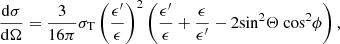 (A.1)
(A.1)
where Θ is the scattering angle, while ϕ is measured from the direction of the photon electric field before scattering (see Fig. 2), and the ratio of photon energies after and before scattering is
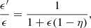 (A.2)
(A.2)
where η = cosΘ, and the photon energies ϵ′ and ϵ are expressed in units of the electron rest mass energy. Integrating Eq. (A.1) over the azimuthal angle one obtains
 (A.3)
(A.3)
which is the well-know formula of the cross-section independent of the polarization state. By substituting Eq. (A.2) into Eq. (A.3) it is possible to derive the non-normalized cumulative probability distribution function of the scattering angle η as a function of the initial photon energy as
![Mathematical equation: $$ \begin{aligned} \mathrm{P}(\epsilon , \eta ) = \frac{3}{8} \sigma _{\rm T}\left[ \frac{ \frac{\epsilon (1-\eta )}{1+\epsilon (1-\eta )}+ \eta ^2 }{1+ \epsilon (1-\eta )]^2}\right]. \end{aligned} $$](/articles/aa/full_html/2025/10/aa54222-25/aa54222-25-eq171.gif) (A.4)
(A.4)
We note that in the limit ϵ → 0 the above formula reduces to P(η) = 3/8σT(1 + η2), the classical Thomson cross-section.
To determine the scattering angle η once given the incident photon energy ϵ, a random number ξ is drawn from uniform distribution over the interval [0-1]. Then, η is found by solving the implicit equation
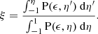 (A.5)
(A.5)
Using the definition of P(ϵ, η) of Eq. (A.4), Eq. (A.5) becomes
![Mathematical equation: $$ \begin{aligned} \begin{aligned} \xi = \frac{1}{\sigma _{\rm tot}(\epsilon )} \Bigg \{\frac{\epsilon ^2}{(-\epsilon \eta +\epsilon +1)^2}-\frac{\epsilon \left(-8 \epsilon ^2+\epsilon +6\right)+2}{(2 \epsilon +1)^2}&\\ +2 \epsilon \eta +\frac{4 \epsilon +2}{-\epsilon \eta +\epsilon +1}+2 [(\epsilon -2) \epsilon -2] \mathrm{Log}\left(\frac{2 \epsilon +1}{ - \epsilon \eta +\epsilon +1}\right) \Bigg \},&\end{aligned} \end{aligned} $$](/articles/aa/full_html/2025/10/aa54222-25/aa54222-25-eq173.gif) (A.6)
(A.6)
where
![Mathematical equation: $$ \begin{aligned} \begin{aligned} \sigma _{\rm tot}(\epsilon ) = \frac{3 }{8 \epsilon ^3} \Bigg \{ \frac{2 \epsilon [2 + \epsilon (1 + \epsilon ) (8 + \epsilon )]}{(1+2 \epsilon )^2}\\ + [\epsilon ^2- 2 \epsilon -2] \mathrm{Log}(1 + 2 \epsilon )\Bigg \}. \end{aligned} \end{aligned} $$](/articles/aa/full_html/2025/10/aa54222-25/aa54222-25-eq174.gif) (A.7)
(A.7)
We note that Eq. (A.6) is not invertible and must be solved numerically. To speed-up computation, we do not solve Eq. (A.6) at each photon-electron scattering event. Instead, we compute a pre-tabulated cumulative matrix Ai, j of scattering angles obtained by numerically solving the equation for a a grid of values ϵi and ξj, in the interval 0.1–105 keV (divided by mec2), and 0–1, respectively. Then, once given ϵ and drawing a random number ξ for each scattering event in the code, the corresponding scattering angle η is obtained by a two-dimensional linear interpolation of the matrix Ai, j.
As it concerns the azimuthal angle ϕ, because each single photon is 100% polarized, after sampling η by solving Eq. (A.6), another random number ξ is drawn and ϕ is derived by inverting the cumulative distribution from Eq. (A.1), which gives (Matt et al. 1996):
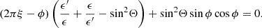 (A.8)
(A.8)
As for Eq. (A.6), this expression must be solved numerically.
Appendix B: Sampling of the Planck distribution using the Debye function
A rejection method to sample photons from a BB spectrum has been presented for example in Pozdnyakov et al. (1983). Here we offer a new method which can be easily implemented especially for the case where built-in libraries such as the GSL are available. The BB photon spectrum is
 (B.1)
(B.1)
With the substitution E ≡ kT, it is possible to rewrite the photon emissivity in adimensional form as
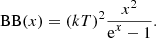 (B.2)
(B.2)
Let us now consider the Debye function of n-order, which is defined as
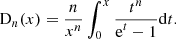 (B.3)
(B.3)
When n = 2, the function within the integral is promptly recognized as the adimensional BB function of Eq. (B.2). The dimensionless photon energy x is selected from the BB distribution by the usual inversion formula for a normalized cumulative distribution:
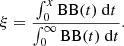 (B.4)
(B.4)
With help of the definition of Dn(x) in Eq. (B.3), Eq. (B.4) can be easily rewritten as
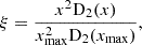 (B.5)
(B.5)
where xmax is chosen sufficiently high so that BB(xmax)→0.
As D2(x) is provided by the GSL, Eq. (B.5) can be numerically solved for instance using a bisection method, and the photon energy in physical units is then simply obtained from E = xkT. Tests performed by sampling a large number of photons showed comparable computational speeds between this and rejection method, albeit the algorithm here proposed is probably easier to be implemented in numericalcodes.
All Tables
Best-fit spectral parameters of the model applied to the IXPE (I, Q, U) and NuSTAR spectra of Cyg X-2 and GX 9+9.
All Figures
|
Fig. 1. Geometrical setup for the bldisk model. Blackbody seed photons from the neutron star are Comptonized in a boundary layer extending up to some latitude (orange region) and characterized by a given electron temperature kTe and optical depth τbl. The other source of thermal photons is the accretion disk, where seed photons are emitted at the top of an electron-scattering atmosphere of optical depth τdisk (green region). Some photons from the disk are Comptonized by the boundary layer, and in turn, the radiation emitted from the latter reaches the disk atmosphere and gets reflected. |
| In the text | |
|
Fig. 2. Geometry for the Cartesian triad attached to a photon directional versor |
| In the text | |
|
Fig. 3. Polarization degree as a function of viewing angle for emerging radiation with seed photons located at the base of a slab with different optical depths. The results were obtained using the iterative method described in F24. Positive and negative values correspond to a PA coplanar with the slab or perpendicular to it, respectively. |
| In the text | |
|
Fig. 4. Example of spectra obtained from the bldisk model, with each free parameter varied in turn. Aside from the individual panels where they are varied, fixed parameters are: θbl = 50°, kTbb = 2 keV, kTe = 3 keV, τbl = 4, ṁ = 1, τdisk = 5, |
| In the text | |
|
Fig. 5. Polarization degree as a function of energy derived from bldisk using the same parameter combination as that reported in Fig. 4. For axisymmetric geometries PD =|Q|, so angle rotation with PA switching from orthogonal (Q > 0) to parallel (Q < 0) direction to the symmetry axis occurs at the energy where PD =0. The vertical lines represent the IXPE energy bands 2–4 keV and 4–8 keV, respectively. |
| In the text | |
|
Fig. 6. Deconvolved EF(E) spectra of IXPE (I, Q, U) and NuSTAR of Cyg X-2 (upper panel) and GX 9+9 (lower panel) with the best-fit model reported in Table 2 superposed and residuals between data and the model in units of σ. The greater rolling angle of Cyg X-2 makes visible the U component of the bldisk spectrum in the IXPE detector reference frame. |
| In the text | |
|
Fig. 7. Polarization degree as a function of energy for Cyg X-2 (upper panel) and GX 9+9 (lower panel) as obtained from the best-fit parameters of Table 2. The two boxes represent the PD boundaries at 3σ confidence level in the 2–4 keV and 4–8 keV energy bands, as measured with the PCUBE algorithm. |
| In the text | |
Current usage metrics show cumulative count of Article Views (full-text article views including HTML views, PDF and ePub downloads, according to the available data) and Abstracts Views on Vision4Press platform.
Data correspond to usage on the plateform after 2015. The current usage metrics is available 48-96 hours after online publication and is updated daily on week days.
Initial download of the metrics may take a while.