| Issue |
A&A
Volume 702, October 2025
|
|
|---|---|---|
| Article Number | A152 | |
| Number of page(s) | 13 | |
| Section | Planets, planetary systems, and small bodies | |
| DOI | https://doi.org/10.1051/0004-6361/202554557 | |
| Published online | 16 October 2025 | |
Six microlensing planets detected via sub-day signals during the 2023–2024 season
1
Department of Physics, Chungbuk National University,
Cheongju
28644,
Republic of Korea
2
Korea Astronomy and Space Science Institute,
Daejon
34055,
Republic of Korea
3
Astronomical Observatory, University of Warsaw,
Al. Ujazdowskie 4,
00-478
Warszawa,
Poland
4
Institute of Natural and Mathematical Science, Massey University,
Auckland
0745,
New Zealand
5
University of Canterbury, Department of Physics and Astronomy,
Private Bag 4800,
Christchurch
8020,
New Zealand
6
Department of Astronomy, Ohio State University,
140 West 18th Ave.,
Columbus,
OH
43210,
USA
7
University of Science and Technology,
Daejeon
34113,
Republic of Korea
8
Department of Particle Physics and Astrophysics, Weizmann Institute of Science,
Rehovot
76100,
Israel
9
Center for Astrophysics | Harvard & Smithsonian
60 Garden St.,
Cambridge,
MA
02138,
USA
10
Department of Astronomy and Tsinghua Centre for Astrophysics, Tsinghua University,
Beijing
100084,
China
11
School of Space Research, Kyung Hee University, Yongin,
Kyeonggi
17104,
Republic of Korea
12
Department of Physics, University of Warwick,
Gibbet Hill Road,
Coventry
CV4 7AL,
UK
13
Villanova University, Department of Astrophysics and Planetary Sciences,
800 Lancaster Ave.,
Villanova,
PA
19085,
USA
14
Institute for Space-Earth Environmental Research, Nagoya University,
Nagoya
464-8601,
Japan
15
Code 667, NASA Goddard Space Flight Center,
Greenbelt,
MD
20771,
USA
16
Department of Astronomy, University of Maryland,
College Park,
MD
20742,
USA
17
Department of Earth and Planetary Science, Graduate School of Science, The University of Tokyo,
7-3-1 Hongo, Bunkyo-ku,
Tokyo
113-0033,
Japan
18
Instituto de Astrofísica de Canarias, Vía Láctea s/n,
38205
La Laguna, Tenerife,
Spain
19
Department of Earth and Space Science, Graduate School of Science, Osaka University,
Toyonaka, Osaka
560-0043,
Japan
20
Department of Physics, The Catholic University of America,
Washington,
DC
20064,
USA
21
Institute of Astronomy, Graduate School of Science, The University of Tokyo,
2-21-1 Osawa,
Mitaka, Tokyo
181-0015,
Japan
22
Sorbonne Université, CNRS, UMR 7095, Institut d’Astrophysique de Paris,
98 bis bd Arago,
75014
Paris,
France
23
Department of Physics, University of Auckland, Private Bag
92019,
Auckland,
New Zealand
24
University of Canterbury Mt. John Observatory,
P.O. Box 56,
Lake Tekapo
8770,
New Zealand
★ Corresponding author: This email address is being protected from spambots. You need JavaScript enabled to view it.
Received:
16
March
2025
Accepted:
4
September
2025
Abstract
Aims. We present analyses of six microlensing events: KMT-2023-BLG-0548, KMT-2023-BLG-0830, KMT-2023-BLG-0949, KMT-2024-BLG-1281, KMT-2024-BLG-2059, and KMT-2024-BLG-2242. These were identified in KMTNet data from the 2023–2024 seasons, selected for exhibiting anomalies shorter than one day – potential signatures of low-mass planetary companions. Motivated by this, we conducted detailed investigations to characterize the nature of the observed perturbations.
Methods. Detailed modeling of the light curves reveals that the anomalies in all six events are caused by planetary companions to the lenses. The brief durations of the anomalies are attributed to various factors: a low planet-to-host mass ratio (KMT-2024-BLG-2059, KMT-2024-BLG-2242), a wide planet-host separation (KMT-2023-BLG-0548), small and elongated caustics restricting the source’s interaction region (KMT-2023-BLG-0830, KMT-2024-BLG-1281), and a partial caustic crossing (KMT-2023-BLG-0949).
Results. We estimated the physical parameters of the lens systems using Bayesian analysis. For KMT-2023-BLG-0548, the posterior distribution of the lens mass shows two distinct peaks: a low-mass solution indicating a sub-Jovian planet orbiting an M dwarf in the Galactic disk, and a high-mass solution suggesting a super-Jovian planet around a K-type dwarf in the bulge. KMT-2023-BLG-0830 hosts a Neptune-mass planet orbiting an M dwarf in the Galactic bulge. KMT-2023-BLG-0949 involves a super-Jovian planet orbiting a ~0.5 M⊙ host located at ~6 kpc. KMT-2024-BLG-2059Lb is a super-Earth with a mass about seven times that of Earth, orbiting an early M dwarf of ~0.5 M⊙. KMT-2024-BLG-1281L hosts a planet slightly more massive than Neptune, orbiting an M dwarf of ~0.3 M⊙. The short timescale and small angular Einstein radius of KMT-2024-BLG-2242 suggest a ~0.07 M⊙ primary, likely a brown dwarf, with a planet of Uranus- or Neptune-like mass.
Key words: gravitational lensing: micro / planets and satellites: detection
© The Authors 2025
 Open Access article, published by EDP Sciences, under the terms of the Creative Commons Attribution License (https://creativecommons.org/licenses/by/4.0), which permits unrestricted use, distribution, and reproduction in any medium, provided the original work is properly cited.
This article is published in open access under the Subscribe to Open model. This email address is being protected from spambots. You need JavaScript enabled to view it. to support open access publication.
1 Introduction
Planetary microlensing signals appear as brief, discontinuous anomalies in the smooth, symmetric lensing light curve of the planet-hosting star (Mao & Paczyński 1991; Gould & Loeb 1992). These signals arise when the source of a lensing event passes close to the caustic induced by the planet. Caustics are regions in the source plane where the magnification of a point source becomes infinite. When a lens system consists of a planet and its host star, two distinct types of caustics form. The first is a small central caustic located near the primary lens, while the second is a peripheral caustic situated at a distance of s − 1/s from the host star. Due to their respective locations, the central caustic produces anomalies near the peak of a high-magnification event light curve, whereas the peripheral caustic primarily generates deviations in the outer regions of the light curve.
The duration of a planetary microlensing signal is primarily determined by the size of the caustic. For peripheral caustics, the caustic size scales with the square root of the planet-to–host mass ratio (Han 2006), whereas for central caustics, it scales linearly with the mass ratio (Chung et al. 2005). As a result, lower-mass planets produce smaller caustics, leading to shorter-duration planetary signals. Therefore, brief planetary anomalies in microlensing light curves are more likely to originate from low-mass planets.
However, short signals in lensing light curves can arise from factors other than the presence of a low-mass planet. For planet–induced caustics, their size depends not only on the mass ratio but also on the projected separation between the planet and its host star. As a result, if this separation deviates significantly from the Einstein radius of the lens, a small caustic may form. Additionally, the signal duration can be shortened if the caustic is highly elongated and the source crosses it along a direction with a small cross-sectional area. A similar effect occurs when the source passes near the edge of the caustic, leading to a reduced signal duration. Moreover, short-term anomalies can also originate from non-planetary causes. One such case involves a binary lens system in which the separation between the two components is either much smaller or much larger than the Einstein radius (Han & Gaudi 2008). It is also well known that a faint companion to the source star can produce a short-term anomaly in the lensing light curve (Gaudi 1998; Gaudi & Han 2004).
In this paper, we analyze six microlensing events: KMT-2023-BLG-0548, KMT-2023-BLG-0830, KMT-2023-BLG-0949, KMT-2024-BLG-1281, KMT-2024-BLG-2059, and KMT-2024-BLG-2242. These events share a common characteristic of displaying anomalies in their light curves that last less than a day. Since such short-term anomalies in a lensing light curve suggest the possible presence of a low-mass planetary companion to the lens, we conducted detailed analyses of these events to investigate the origin and nature of the anomalies.
For the presentation of the analyses, the paper is structured as follows. In Sect. 2, we outline the process of identifying the anomalies in the lensing light curves of the events analyzed in this study, along with the data employed for the analysis. In Sect. 3, we provide an overview of the fundamentals of planetary microlensing and detail the modeling procedure employed to interpret the anomalies observed in the lensing light curves. Within the six subsections of Sect. 4, we present the modeling results for each individual event and discuss the origins of the anomalies. In Sect. 5, we characterize the source stars for each event and determine the angular Einstein radii for the events for which finite-source effects were detected. In Sect. 6, we estimate the masses and distances of the lens systems by performing Bayesian analyses based on the observables derived from the analyses. Finally, in Sect. 7, we summarize the findings and present our conclusions.
2 Observations and data
The lensing events analyzed in this study were identified by examining microlensing events detected by the Korea Microlensing Telescope Network (KMTNet; Kim et al. 2016) during the 2023 and 2024 seasons. The goal was to identify lensing events that displayed very short-term anomalies in their light curves. From this examination, we found six lensing events, KMT-2023-BLG-0548, KMT-2023-BLG-0830, KMT-2023-BLG-0949, KMT-2024-BLG-1281, KMT-2024-BLG-2059, and KMT-2024-BLG-2242, that each displayed short-term anomalies lasting less than a day. These events were found with the application of the KMTNet EventFinder system (Kim et al. 2018) applied to the KMTNet data acquired during the corresponding seasons. The anomalies in these events were identified with the use of the semi-automatic AnomalyFinder algorithm (Zang et al. 2021).
We examined the availability of additional data from other microlensing surveys. Among the events identified by the KMTNet survey, KMT-2023-BLG-0949 and KMT-2024-BLG-2059 were also observed by the Optical Gravitational Lensing Experiment (OGLE; Udalski et al. 2015), while KMT-2024-BLG-1281 was observed by the Microlensing Observations in Astrophysics (MOA; Bond et al. 2001; Sumi et al. 2003). KMT-2024-BLG-2242 was covered by both the OGLE and MOA surveys. For these events, we carried out the analysis using the combined data sets from the respective surveys.
The data for the events were acquired using wide-field telescopes of the survey groups specifically designed for microlensing surveys. The KMTNet group operates three identical telescopes strategically positioned across the Southern Hemisphere to facilitate continuous observations. These telescopes are located at the Siding Spring Observatory in Australia (KMTA), the Cerro Tololo Inter-American Observatory in Chile (KMTC), and the South African Astronomical Observatory in South Africa (KMTS). Each KMTNet telescope features a 1.6-meter aperture and is equipped with a camera that provides a field of view of 4 square degrees. The OGLE telescope, situated at the Las Campanas Observatory in Chile, has a 1.3-meter aperture and a camera offering a field of view of 1.4 square degrees. The MOA survey conducts observations using a 1.8-meter telescope stationed at Mt. John University Observatory in New Zealand, featuring a wide-field camera capable of imaging an area of 2.2 square degrees in a single exposure.
The KMTNet and OGLE surveys primarily conducted observations in the I band, whereas the MOA survey used a custom MOA-R filter, which covers a wavelength range of 609–1109 nm. In all three surveys, a subset of images was also taken in the V band to enable the measurement of source colors. The photometry of the events was conducted using the pipelines of the respective groups. To ensure the optimal quality of data, the KMTNet data were reprocessed using the code developed by Yang et al. (2024). The photometric errors estimated by the automated pipeline were rescaled to align the errors with the observed scatter in the data and to ensure that the χ2 value of the model matched unity for each dataset. This rescaling procedure was performed in accordance with the methodology outlined in Yee et al. (2012).
3 Light curve modeling
The modeling process involved determining the lensing parameters that best characterize the observed lensing light curves. For a single-lens single-source (1L1S) event, the light curve is described by three parameters. The first two parameters, (t0, u0), represent the time of the closest approach between the lens and source and their separation at that moment. The third parameter, tE, denotes the event timescale, which is defined as the duration required for the source to traverse the Einstein radius (θE) of the lens. The parameter u0 is expressed in units of θE.
For a binary-lens single-source (2L1S) event, which includes an additional lens component compared to the 1L1S case, four additional parameters (s, q, α, ρ) are required for modeling. Here, s and q represent the projected separation and mass ratio between the two lens components, respectively. The parameter α denotes the angle between the source trajectory and the binary lens axis, while ρ is the ratio of the angular source radius (θ*) to the Einstein radius, given by ρ = θ*/θE. The parameter ρ is necessary to account for finite-source effects, which arise when the source passes very close to or crosses the caustic, a frequent characteristic feature of 2L1S events. The binary separation s is expressed in units of θE.
Similar to the 2L1S case, modeling a single-lens binary-source (1L2S) event requires additional parameters. These parameters are (t0,2, u0,2, qF), where the first two parameters denote the approach time and separation of the second source relative to the lens, respectively, while the last parameter represents the flux ratio between the secondary and primary sources (Hwang et al. 2013). For a summary of lensing parameters across different lens-system configurations, refer to Table 2 of Han et al. (2023).
The 2L1S modeling was conducted using a hybrid approach that combines grid and downhill optimization methods. Due to the large number of model parameters, it is challenging to identify a lensing solution using a purely grid-based approach. Therefore, we explored the parameter space for s and q, for which the lensing magnification changes abruptly with variations in these parameters, using a grid approach, while the remaining parameters, for which magnification varies smoothly, were optimized using downhill methods with multiple starting values of α. Another reason for using the grid approach to search for s and q is to identify degenerate solutions that might be present in the plane of these parameters. To compute finite-source magnifications, we employed the map-making technique based on the ray-shooting method (Dong et al. 2006). In this process, variations in the surface brightness profile of the source star due to limb darkening were taken into account by considering the spectral type of the star. Details on the determination of the source type are provided in Sect. 5.
The 1L2S modeling was carried out by first applying 1L1S modeling to the light curve while excluding the part around the anomaly. In the next step, the binary-source parameters responsible for the anomaly were determined using a downhill approach, with initial parameters set based on the strength and time of the anomaly.
4 Analyses of individual events
In the following subsections, we provide a detailed analysis of each individual event and present the results obtained. For cases with multiple possible interpretations, we discuss the sources of the degeneracy.
4.1 KMT-2023-BLG-0548
The lensing event KMT-2023-BLG-0548 occurred on a faint star at equatorial coordinates (RA, Dec)J2000 = (18:01:23.43, −27:06:24.30), corresponding to Galactic coordinates (l, b) = (3°.3426, −2°.0710). The I-band extinction toward this field is AI = 2.24, and the baseline source magnitude prior to lensing magnification was Ibase = 20.01.
The KMTNet survey first detected the lensing-induced flux magnification of the source on 2023 April 24 (corresponding to the abridged Heliocentric Julian Date HJD′ ≡ HJD − 2 460 000 = 58), two days after the event had reached its very high peak magnification of Amax ~ 940. The source lies in the overlapping region of the KMTNet prime fields BLG03 and BLG43, which were observed with a cadence of 0.5 hours per field, corresponding to a combined cadence of 0.25 hours.
Figure 1 shows the lensing light curve of the event, which appears consistent with a high-magnification 1L1S event. However, model fitting to the 1L1S framework revealed subtle deviations near the peak of the light curve. These anomalies were brief, lasting only several hours, and were captured by KMTA observations from the BLG43 field. Although the BLG03 field also covered the peak region, its data were excluded from the analysis due to large photometric uncertainties.
Since a central anomaly in a lensing light curve can be attributed either to a planet orbiting the lens (Griest & Safizadeh 1998) or to a binary companion located either close to or far from the lens (Han & Gaudi 2008), we conducted 2L1S modeling of the light curve. This analysis resulted in four sets of planetary solutions, with the full lensing parameters provided in Table 1. The first two solutions share a similar source trajectory angle of α ~ 2.27 radians (local A), while the other two have an angle of α ~ 0.16 radians (local B), suggesting that the degeneracy between solutions in the local A and B groups is coincidental. In contrast, the planetary separations within each local group follow the relation sclose ~ 1/swide, implying that the similarity between the model light curves of the degenerate solutions is a result of the close-wide degeneracy (Dominik 1999). Here, the terms “close” and “wide” refer to solutions with s < 1 and s > 1, respectively. Regardless of the specific solution, the estimated event timescale is ~25 days, and the planet-to-host mass ratios are on the order of 10−3, indicating that the companion to the lens is likely a planetary object.
In the top panels of Figure 1, we present the model curves for the solutions in the region surrounding the anomaly. For each pair of local A and B solutions, we display the model curve of the close solution as the representative, since the model light curves from the close and wide solutions are nearly identical. In contrast, the model curves for the local A and B solutions start to diverge beyond HJD′ ≥ 53.32, a time interval during which no data were available to constrain the anomaly. This divergence provides further confirmation that the degeneracy between the two solutions is accidental, and the ambiguity could have been resolved if the observations had extended to this region, which would have allowed for a clearer distinction between the solutions.
The four insets in the bottom panel of Figure 1 depict the lens system configurations, illustrating the trajectory of the source with respect to the caustic induced by the planet. In all degenerate solutions, the planet generates a very small central caustic, with a size less than 0.4% of the Einstein radius. As a result, the anomaly lasted for a very short duration. The size of the central caustic depends on both the planetary separation s and the mass ratio q, shrinking as s deviates from unity and as q decreases (Chung et al. 2005). Given the estimated mass ratio of q ~ 4 × 10⁻³, which corresponds to that of a giant planet orbiting a normal star, the short duration of the anomaly is attributed to the significant deviation of s from unity. In all solutions, the size and shape of the induced caustic are similar. However, for the Local A solutions, the source crosses the planet-star axis at an angle of about 41°, while for the Local B solutions, the angle is smaller, around 9°. Because the source is relatively large compared to the caustic, significant finite-source effects occur. Consequently, even though the source passes through the caustic, the resulting distortion is relatively small due to these substantial finite-source effects (Bennett & Rhie 1996).
We also considered a model under a 1L2S configuration. The best-fit parameters for the 1L2S model are listed in Table 1, and the corresponding model curve, along with its residuals, is shown in Figure 1. From the comparison of fits, it was found that the 1L2S model provides a poorer fit compared to the 2L1S model, with a χ2 difference of 12.6, indicating that the 1L2S solution is less favored relative to the 2L1S model.
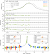 |
Fig. 1 Light curve of the microlensing event KMT-2023-BLG-0548. The bottom panel displays the full light curve, while the upper panels present a zoomed-in view of the peak region along with the residuals for four different models. The four insets in the bottom panel illustrate the lens-system configurations corresponding to the four degenerate 2L1S solutions. In each inset, the closed figure composed of concave curves represents the caustics, and the arrowed line indicates the source trajectory. The orange circle, scaled to represent the angular size of the source, on the trajectory marks the source’s position at the moment of peak anomaly. |
Lensing parameters of solutions for KMT-2023-BLG-0548.
4.2 KMT-2023-BLG-0830
The source of the event KMT-2023-BLG-0830 is located at (RA, Dec)J2000 = (18:06:37.91, −28:19:56.32), corresponding to Galactic coordinates (l, b) = (2°.8407, −3°.6823). The source has a baseline I-band magnitude of Ibase = 20.40, with an extinction of AI = 1.01 in this direction. The event was exclusively observed by the KMTNet survey, which first detected the lensing-induced magnification on 2023 May 15 (HJD′ = 79), approximately three days before the peak. The source lies in the overlapping region of the BLG03 and BLG32 fields, which were monitored with cadences of 0.5 hours and 2.5 hours, respectively.
Figure 2 presents the lensing light curve of KMT-2023-BLG-0830, which, at first glance, appears to correspond to a standard 1L1S event with a high peak magnification of approximately Amax ~ 50. However, a detailed examination of the peak region of the light curve revealed the presence of a subtle anomaly occurred at around HJD′ ~82.42. This anomaly, which has a very short duration of about 1.2 hours, was covered by the data obtained from KMTC observations.
Given the abrupt change in lensing magnification during the anomaly and its occurrence near the peak of the light curve, we modeled the event under a 2L1S configuration. This analysis identified two degenerate solutions resulting from the close-wide degeneracy. From the modeling, we estimated the mass ratio between the lens components to be approximately q ~ 0.25 × 10⁻³, indicating that the companion to the lens is a low-mass planetary object. The full sets of lensing parameters for both solutions, along with their corresponding χ2 values, are presented in Table 2. The degeneracy between the two solutions is very severe, with only a marginal difference of Δχ2 = 0.2. As we discuss below, the anomaly was caused by the source crossing a central caustic induced by the planet. However, due to the limited coverage of the anomaly, the normalized source radius could not be securely determined.
Figure 2 presents the model light curves and residuals for the two degenerate 2L1S solutions, while the insets in the bottom panel illustrate the corresponding lens system configurations. The configurations reveal that the planet generated a small central caustic that is elongated along the planet–host axis, and the anomaly occurred as the source passed diagonally through this axis. The short duration of the anomaly resulted from a combination of factors, including the small caustic size, which is primarily due to the low planetary mass ratio, and the elongated shape of the caustic, which reduced the cross-sectional area traversed by the source. In the close solution, the peripheral caustic, which is substantially larger than the central caustic, forms on the opposite side of the planet, whereas in the wide solution, it appears on the same side as the planet. However, these peripheral caustics are located at a considerable distance from the source trajectory and have no impact on the planetary perturbation.
We found that the 1L2S interpretation is disfavored relative to the planetary interpretation. This is illustrated in Figure 2, which displays the model derived under the 1L2S configuration along with its residuals. The lensing parameters for the 1L2S solution are detailed in Table 2. The analysis reveals that the 1L2S model provides a worse fit than the planetary solution, with a Δχ2 = 15.7. Upon examining the residuals, it is evident that the 1L2S model fails to adequately account for the negative deviation observed after the main anomaly feature.
Lensing parameters of solutions for KMT-2023-BLG-0830.
4.3 KMT-2023-BLG-0949
The lensing event KMT-2023-BLG-0949 was observed not only by the KMTNet survey but also through additional observations conducted by the OGLE group. The KMTNet survey first detected the event on 2023 April 24 (HJD′ = 86) during its rising phase, while the OGLE survey reported the discovery of the event a week later. The OGLE ID reference of the event is OGLE-2023-BLG-0581. Hereafter, we refer to the event using the KMTNet ID, following the microlensing community’s convention of adopting the designation from the survey group that first discovered the event. The equatorial and Galactic coordinates of the event are (RA, DEC)J2000 = (17:33:40.66, -28:05:29.26) and (l, b) = (−0°.6798,2°.67087), respectively. The baseline magnitude of the source is Ibase = 19.6, and the extinction toward the field is AI = 2.72. The event peaked at HJD′ ~ 93.2, reaching a relatively high magnification of Apeak ~ 40. The source is located in the KMTNet BLG14 field, where observations were carried out with an hourly cadence.
Figure 3 presents the lensing light curve of KMT-2023-BLG-0949, which exhibits an anomaly near the peak with a duration of less than a day. The main portion of the anomaly was covered by the KMTC data, while its declining phase was captured by the KMTA data. A detailed examination of the residuals from a 1L1S model revealed the presence of additional weak negative deviations in an extended region centered at around HJD′ = 90.
From the 2L1S modeling of the light curve, we identified two solutions resulting from the close-wide degeneracy. The complete lensing parameters for these solutions are presented in Table 3. The estimated mass ratio between the lens components is q = (11.77 ± 1.02) × 10−3 for the close solution and q = (7.69 ± 0.65) × 10−3 for the wide solution, indicating that the companion to the lens is a giant planet. The model curves for the two solutions in the region around the anomaly are shown in the top panel of Figure 3. It is found that the close solution is preferred over the wide solution by Δχ2 = 15.7. A notable point is that the models in the region not covered by the data are substantially different, suggesting that the degeneracy between the two solutions could have been resolved if the sky at the KMTA sites on the night of HJD′ = 93 (2023 May 28) had not been clouded out. Due to the partial coverage of the anomaly, the normalized source radius could not be securely constrained, and only its upper limit (ρmax ~ 3 × 10⁻³) is determined. Modeling the anomaly under a 1L2S configuration results in a solution that is significantly worse than the planetary solution, with a Δχ2 of 244.2.
The lens-system configurations for the close and wide solutions are displayed in the two insets within the bottom panel of Figure 3. Unlike previous events, KMT-2023-BLG-0949 reveals that the central caustics of the close and wide solutions exhibit less similarity. In the close solution, the central caustic and the peripheral caustic are clearly separated, whereas in the wide solution, the two caustics merge to form a single large resonant caustic. In both cases, the anomaly occurred when the source crossed the upper left tip of the central caustic. Despite the relatively large size of the caustic, the anomaly had a short duration because the source traversed only a small portion of it. Additionally, the weak negative deviation observed before the peak resulted from the source passing through the extended negative deviation region on the back side of the central caustic. Similar planetary signals with extended weak negative deviations have been observed in four previously reported planetary lensing events: KMT-2020-BLG-0757, KMT-2022-BLG-0732, KMT-2022-BLG-1787, and KMT-2022-BLG-1852 (Han et al. 2024a).
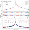 |
Fig. 3 Light curve of KMT-2023-BLG-0949. We note that in addition to the strong anomaly near the peak, there are also additional weak extended negative deviations in the rising part of the light curve. |
Lensing parameters KMT-2023-BLG-0949.
4.4 KMT-2024-BLG-1281
The lensing event KMT-2024-BLG-1281 occurred on a faint source with an I-band baseline magnitude of Ibase = 19.70. It was first identified by the KMTNet survey on June 4, 2024 (HJD′ = 465), during the rising part of the light curve, and was later confirmed by the MOA survey, which designated the event as MOA-2024-BLG-077. The equatorial and Galactic coordinates of the event are (RA, DEC)J2000 = (11:00:40.65, −32:42:51.30) and (l, b) = (−1°.6220, −4°.7000), respectively. The event lies within the KMTNet BLG34 field, which is characterized by relatively low extinction (AI = 1.04) compared to other KMTNet fields. This field was monitored at a cadence of 2.5 hours. The event reached a relatively high magnification of Amax ~ 25 at HJD′ ~ 480.9.
The peak region of a high-magnification event is sensitive to perturbations caused by a planetary companion. Upon examining the light curve with this in mind, we identified a short-lived anomaly lasting less than a day, centered around HJD′ ~ 481.2. Figure 4 presents the light curve of KMT-2024-BLG-1281, with the lower panel displaying the full view and the upper panel providing a zoomed-in view of the anomaly region. One KMTS data point at HJD′ = 481.269 shows a negative deviation from the 1L1S model, while two other points – a MOA point at HJD′ = 480.927 and a KMTS point at HJD′ = 481.423 – exhibit positive deviations relative to the 1L1S model. Besides these points, the KMTC point at HJD′ = 60480.698 appears to slightly deviate from the 1L1S model.
Light curve modeling under the 2L1S configuration revealed three degenerate solution sets. In all cases, the mass ratio between the lens components is approximately q ~ 2 × 10⁻⁴, indicating that the companion is planetary in nature. For each solution, the normalized separation between the lens components is close to unity, implying that the planet resides near the Einstein ring. The complete set of lensing parameters for each solution is listed in Table 4. The solutions are referred to as “inner,” “outer,” and “intermediate,” as described in the discussion below. The top panel of Figure 4 presents the model light curves for the three solutions, along with their corresponding residuals. The intermediate solution yields a better fit than the inner and outer solutions, with improvements of Δχ2 = 11.7 and 12.2, respectively. The normalized source radius could not be constrained because the anomaly was sparsely covered.
The insets within the bottom panel of Figure 4 displays the lens-system configurations corresponding to the three solutions. According to the inner solution, the source passed through the inner side of the peripheral caustic relative to the planet host, while for the outer solution, the source trajectory lay on the outer side of the caustic. In the intermediate solution, the source crossed directly over the caustic. Based on these configurations, we label the solutions as “inner,” “outer,” and “intermediate,” respectively. The degeneracy between the inner and outer solutions was first identified by Gaudi & Gould (1997), who described it as arising from source trajectories that pass on opposite sides – inner and outer – of a planetary caustic. Yee et al. (2021) and Zhang et al. (2022) later demonstrated that this type of degeneracy can also occur in planetary perturbations induced by both central and planetary caustics. Subsequently, Hwang et al. (2022) and Gould et al. (2022) proposed analytic relations linking the planetary parameters of the degenerate solutions. For all solutions, the source trajectory passes nearly vertically through the perturbation region, which is elongated along the planet-host axis. Combined with the small caustic size generated by the low-mass planet, this results in a short-duration perturbation.
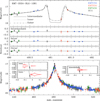 |
Fig. 4 Light curve of the lensing event KMT-2024-BLG-1281. |
Lensing parameters of solutions for KMT-2024-BLG-1281.
4.5 KMT-2024-BLG-2059
The microlensing event KMT-2024-BLG-2059 occurred on a source with a baseline magnitude of Ibase = 18.12, located at equatorial coordinates (RA, DEC)J2000 = (18:03:43.14, −28:34:05.48), corresponding to Galactic coordinates (l, b) = (2°.3220, −3°.2378). The event was first detected by the KMTNet survey on 2024 August 5 (HJD′ = 527), two days prior to its peak. It was later independently identified by the OGLE survey on August 16 (HJD′ = 538) and designated as OGLE-2024-BLG-1095. The source lies in the overlapping region of the two KMTNet prime fields, BLG03 and BLG43, which were monitored with a combined cadence of 0.25 hours. This region is located near Baade’s Window, where the extinction is relatively low (AI = 0.96).
Figure 5 shows the lensing light curve of the event. Modeling under the 1L1S configuration revealed that the observed flux is substantially influenced by blended light. As a result, although the event reached a relatively high magnification of Amax ~ 20, the source brightened by only ~0.52 magnitudes above the baseline at the peak. Due to the sensitivity of high-magnification events to planetary perturbations, we examined the peak region of the light curve. This examination revealed a brief anomaly lasting about 9 hours, as displayed in the top panel of Figure 5. The anomaly, captured by two KMTS data sets, displays a negative deviation from the 1L1S model. As demonstrated by the recently reported planetary events MOA-2022-BLG-033Lb, KMT-2023-BLG-0119Lb, and KMT-2023-BLG-1896Lb (Han et al. 2025), such short-duration dips near the peak of a high-magnification event are strong indicators of a planetary origin.
Detailed modeling of the light curve confirmed the planetary nature of the anomaly. The analysis yielded two local solutions arising from the inner-outer degeneracy. The planet parameters are (s, q) ~ (0.94, 3.9 × 10⁻⁵) for the inner solution and (1.02, 4.0 × 10⁻⁵) for the outer solution. The full sets of lensing parameters for both solutions are listed in Table 5. We exclude the 1L2S interpretation, as perturbations induced by a source companion always produce positive deviations. The model curves for the two solutions, along with their residuals, are presented in the upper panels of Figure 5. The fits are nearly indistinguishable, with a χ2 difference of only Δχ2 = 0.23.
The two insets in the bottom panel of Figure 5 illustrate the lens-system configurations corresponding to the inner and outer solutions. As in the case of KMT-2024-BLG-1281, the source trajectory passes through the inner side of the peripheral caustic in the inner solution and through the outer side in the outer solution. The dip-like anomaly arose as the source crossed a region of negative deviation located on the backside of the central caustic along the planet–host axis. The short duration of the perturbation results from the nearly vertical source trajectory across the anomaly region, combined with the small caustic size produced by the low-mass planet. The normalized source radius could not be constrained, as the source did not intersect the caustic.
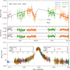 |
Fig. 5 Lensing light curve of the event KMT-2024-BLG-2059. |
Lensing parameters KMT-2024-BLG-2059.
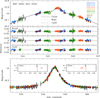 |
Fig. 6 Lensing light curve of KMT-2024-BLG-2242. |
4.6 KMT-2024-BLG-2242
The lensing event KMT-2024-BLG-2242 occurred on a source with a relatively bright baseline magnitude of Ibase = 16.68. The source is located at equatorial coordinates (RA, DEC)J2000 = (17:53:39.60, −29:33:37.12) and Galactic coordinates (l, b) = (0°.3655, −1°.8252). The extinction toward this field is AI = 1.84. The event was independently identified in its early phase by all three active microlensing surveys. KMTNet and MOA detected it on the same day, August 19 (HJD′ = 541), while OGLE reported the detection several days later. We adopt the KMTNet designation for the event. The corresponding event IDs from the MOA and OGLE surveys are MOA-2024-BLG-204 and OGLE-2024-BLG-1122, respectively. The event reached a peak magnification of Amax ~ 2.3 at HJD′ = 545.2. Although the timescale was short, tE ~ 4.6 days as derived from a 1L1S model fit, the light curve was densely covered thanks to the event’s location in KMTNet prime fields BLG02 and BLG42, which were monitored with a combined cadence of 15 minutes.
The lensing light curve of KMT-2024-BLG-2242 is shown in Figure 6. Although it initially resembles a standard 1L1S event, a closer inspection of the peak region reveals a brief anomaly lasting less than a day. This deviation, captured by the combined KMTS, KMTC, and OGLE data sets, appears as a bump with a positive deviation from the 1L1S model. If this anomaly is attributed to a planetary companion, its short duration suggests the presence of a low-mass planet. In such a case, it is unlikely that the perturbation was caused by the central caustic, as the central caustic induced by a low-mass planet is too small to generate a signal at low magnification. A more plausible interpretation is that the bump-like anomaly resulted from the source passing nearly perpendicularly through the perturbation region associated with the peripheral caustic.
Detailed modeling confirms the planetary origin of the anomaly. We identified two degenerate solutions resulting from the inner-outer degeneracy. The planetary parameters are approximately (s, q) ~ (1.35, 7.5 × 10⁻⁴) for the inner solution and (s, q) ~ (1.18, 6.0 × 10⁻⁴) for the outer solution, indicating that the companion is a low-mass planet. The complete parameter sets for both solutions are provided in Table 6, and the corresponding model curves and residuals are presented in the upper panels of Figure 6. The two solutions are very degenerate, with the outer solution being slightly favored by Δχ2 = 4.2.
We also considered the possibility that the anomaly was caused by a binary companion to the source. Modeling under a 1L2S configuration produced a fit comparable to those of the planetary models. The full set of parameters for the 1L2S solution is presented in Table 6. According to this model, the source companion is extremely faint, with a flux ratio to the primary of qF ~ 2 × 10⁻³. However, the inferred normalized source radius, ρ2 ~ 30 × 10−3, corresponds to that of a giant star. This inconsistency between the companion’s faintness and its large angular size is physically implausible, leading us to reject the 1L2S interpretation for the anomaly.
The lens-system configurations corresponding to the inner and outer planetary solutions are presented in the two insets within the bottom panel of Figure 6. As anticipated from the heuristic analysis, the anomaly was caused by the source passing nearly vertically through the perturbation region induced by the peripheral caustic. In the inner solution, the source trajectory passes on the inner side of the caustic, while in the outer solution, it passes on the outer side. The short duration of the anomaly is primarily due to the small size of the caustic, which results from the low planet-to-host mass ratio. Although the source does not cross the caustic in either solution, the normalized source radius was nonetheless constrained, albeit with relatively large uncertainty. This was made possible by the substantial angular size of the source, as discussed in the following section.
5 Source stars
Identifying the source of a lensing event is essential not only for fully characterizing the event but also for estimating the angular Einstein radius. Determining the source type allows one to estimate the angular source radius, θ*. With this value, the angular Einstein radius can be calculated using the relation
![Mathematical equation: $\[\theta_{\mathrm{E}}=\frac{\theta_*}{\rho},\]$](/articles/aa/full_html/2025/10/aa54557-25/aa54557-25-eq1.png) (1)
(1)
where ρ is the normalized source radius, derived from modeling events that exhibit measurable finite-source effects. Among the analyzed events, ρ was reliably measured for KMT-2023-BLG-0548, KMT-2024-BLG-1281, and KMT-2024-BLG-2242, allowing for the estimation of the angular Einstein radius, θE. For KMT-2023-BLG-0949, only an upper limit on ρ could be determined, which in turn provides a lower limit on θE.
To determine the source type, we began by estimating the instrumental color and magnitude. This was achieved by regressing the observed flux Fobs(t) in the I and V passbands against the model magnification Amodel(t);
![Mathematical equation: $\[F_{\text {obs }}(t)=A_{\text {model }}(t) F_s+F_b,\]$](/articles/aa/full_html/2025/10/aa54557-25/aa54557-25-eq2.png) (2)
(2)
where Fs and Fb represent the flux values of the source and the blend, respectively. The instrumental color and magnitude, (V − I, I)s, were subsequently calibrated using the method described by Yoo et al. (2004), which employs the centroid of the red giant clump (RGC) in the color-magnitude diagram (CMD) as a reference. The RGC centroid serves as a reference for calibration because its de-reddened color and magnitude, (V − I, I)RGC,0, are known in previous studies by Bensby et al. (2013) and Nataf et al. (2013). By measuring the offsets Δ(V − I, I) between the source and the RGC centroid in the instrumental CMD, the de-reddened values of the source are determined as
![Mathematical equation: $\[(V-I, I)_{s, 0}=(V-I, I)_{\mathrm{RGC}, 0}+\Delta(V-I, I).\]$](/articles/aa/full_html/2025/10/aa54557-25/aa54557-25-eq3.png) (3)
(3)
Figure 7 shows the positions of the source stars relative to the RGC centroids on the instrumental CMDs, constructed from stars located near the source in each event. For events with measured blended flux, we also indicate the positions of the blend. The CMDs were generated using photometry performed with the pyDIA photometry code (Albrow et al. 2017), which was also used to measure the source color. The estimated values of (V − I, I)s, (V − I, I)RGC, (V − I, I)RGC,0, and (V − I, I)s,0 are presented in Table 7. With the exception of KMT-2024-BLG-2242, the measured colors and magnitudes indicate that the source stars are main-sequence stars with spectral types ranging from mid-G to early-M. In the case of KMT-2024-BLG-2242, the source is identified as a K-type giant with a much larger angular radius than those of the other events. This accounts for the ability to measure the normalized source radius in this case, even though the source passed the caustic at a relatively large separation.
The angular source radius was estimated using the measured color and magnitude of the source star, based on the empirical relation of Kervella et al. (2004), which links (V − K, I) to θ*. Because this relation requires (V − K, K) as input, the observed (V − I, I) values were converted to (V − K, K) using the color-color transformation provided by Bessell & Brett (1988). With the derived angular source radius, the angular Einstein radius, θE, was computed using Equation (1). The relative lens-source proper motion, μ, was then obtained from the event timescale, tE, determined through modeling, via the relation μ = θE/tE.
The resulting values of θE and μ are summarized in Table 8 for the three events exhibiting finite-source effects: KMT-2023-BLG-0548, KMT-2024-BLG-1281, and KMT-2024-BLG-2242. For KMT-2023-BLG-0949, where only an upper limit on ρ could be constrained, lower limits on θE and μ are provided. Notably, the angular Einstein radius measured for KMT-2024-BLG-2242, θE = 0.090 ± 0.021 mas, is significantly smaller than those of the other events. Combined with its short timescale of tE = 4.687 ± 0.068 days, this indicates that the lens likely has a very low mass.
Lensing parameters KMT-2024-BLG-2059.
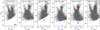 |
Fig. 7 Locations of source stars (blue dots) with respect to the centroid of the red giant clump (RGC, red dots) in the instrumental color-magnitude diagrams of the six planetary lensing events. For events with measured blended flux, the positions of the blend (green dots) are also indicated. |
Source parameters.
Angular Einstein radii.
6 Physical lens parameters
The physical parameters of the lens, including its mass (M) and distance (DL), were determined by performing a Bayesian analysis. This analysis incorporated priors based on the Galactic model and the mass function of Galactic objects, along with constraints provided by the measured lensing observables. The lensing observables that provide constraints on M and DL are the event timescale tE, the angular Einstein radius θE, and the microlens parallax πE because they are related to the physical parameters through the following relations:
![Mathematical equation: $\[t_{\mathrm{E}}=\frac{\theta_{\mathrm{E}}}{\mu}, \quad \theta_{\mathrm{E}}=\left(\kappa M \pi_{\mathrm{rel}}\right)^{1 / 2}, \quad \pi_{\mathrm{E}}=\frac{\pi_{\mathrm{rel}}}{\theta_{\mathrm{E}}}.\]$](/articles/aa/full_html/2025/10/aa54557-25/aa54557-25-eq4.png) (4)
(4)
Here κ = 4G/c2AU) ≃ 8.144 mas/M⊙, πrel = AU(1/DS − 1/DS) represents the relative lens-source parallax, and DS is the distance to the source. With the complete measurements of these observables, the lens mass and distance can be uniquely determined using the relations
![Mathematical equation: $\[M=\frac{\theta_{\mathrm{E}}}{\kappa \pi_{\mathrm{E}}}; \quad D_{\mathrm{L}}=\frac{\mathrm{AU}}{\pi_{\mathrm{E}} \theta_{\mathrm{E}}+\pi_{\mathrm{S}}},\]$](/articles/aa/full_html/2025/10/aa54557-25/aa54557-25-eq5.png) (5)
(5)
where πS = AU/DS. However, in none of the observed events were all three lensing observables measured in full. As a result, we inferred the physical parameters by performing a Bayesian analysis. This approach incorporates not only the constraints from the measured observables but also prior information based on the physical and dynamical distributions of lenses, as well as their mass function.
The Bayesian analysis commenced with the generation of a large set of synthetic lensing events. The physical parameters of each synthetic event, (Mi, DL,i, DS,i, μi), were assigned using a Monte Carlo simulation based on a prior Galactic model and lens mass function. For the Galactic model, which describes the physical and dynamical distributions of lensing objects in the Galaxy, we adopted the model outlined in Jung et al. (2021). In this model, the Galaxy is basically represented as a triaxial bulge plus a double-exponential disk with some refinement based on Gaia data and observed disk rotation curve. For the lens mass function, which characterizes the distributions of lens masses, we employed the model detailed in Jung et al. (2022), which includes contribution from stars, brown dwarfs, and remnants (white dwarfs, neutron stars, and black holes). For each synthetic event, we calculated the lensing observables corresponding to the assigned physical parameters using the relations in Eq. (4). Based on the ensemble of generated synthetic events, the posterior probability distributions of the lens mass, M and distance, DL, were derived by weighting each event according to its consistency with the observed lensing observables. The applied weight accounts for how well the simulated observables match the measured values and is defined as
![Mathematical equation: $\[w_i=\exp \left(-\frac{\chi_i^2}{2}\right); \quad \chi_i^2=\frac{\left(t_{\mathrm{E}, i}-t_{\mathrm{E}}\right)^2}{\sigma\left(t_{\mathrm{E}}\right)^2}+\frac{\left(\theta_{\mathrm{E}, i}-\theta_{\mathrm{E}}\right)^2}{\sigma\left(\theta_{\mathrm{E}}\right)^2}.\]$](/articles/aa/full_html/2025/10/aa54557-25/aa54557-25-eq6.png) (6)
(6)
Here, (tE, θE) are the observed Einstein timescale and angular Einstein radius, and σ(tE), σ(θE) denote their respective uncertainties. For events without a measured θE, the second term in the χ2 calculation in Eq. (6) is not included.
Figures 8 and 9 present the posterior distributions of the lens mass and distance obtained from the Bayesian analysis. The estimated physical parameters, including Mh, Mp, DL, and a⊥, are summarized in Table 9. Here, Mh and Mp represent the masses of the host star and planet, respectively, while a⊥ denotes the projected separation between the planet and its host. The median value of each parameter was adopted as the representative estimate, with the lower and upper limits defined by the 16th and 84th percentiles of the posterior distribution, respectively. The tables also provide the probabilities of the lens residing in the Galactic disk (pdisk) or bulge (pbulge).
For KMT-2023-BLG-0548, the posterior distribution of the lens mass reveals two distinct peaks: one at M1 ~ 0.12 M⊙ (low-mass peak) and another at M1 ~ 0.72 M⊙ (high-mass peak). To account for this bimodal distribution, we separately estimated the physical parameters associated with each peak. Based on the posterior distribution near the low-mass peak, the planetary companion is estimated to have a sub-Jovian mass of approximately 0.6 MJ. In contrast, the posterior distribution near the high-mass peak suggests a significantly more massive planet, with a super-Jovian mass of approximately 3.5 MJ. The host star associated with the low-mass peak is an M dwarf located in the Galactic disk, whereas the host corresponding to the high-mass peak is a K-type dwarf situated in the Galactic bulge.
For the event KMT-2023-BLG-0830, the lens system consists of a planet with a mass of approximately ~0.06 MJ, comparable to the mass of Neptune in the solar system, and a host star with a mass of approximately ~0.22 M⊙, corresponding to a mid-M dwarf. The estimated distance to the system, DL ~ 7.3 kpc, strongly suggests that this planetary system is likely located in the Galactic bulge.
The companion of KMT-2023-BLG-0949L is a giant planet with an estimated mass of about ~6 MJ for the close solution and ~4 MJ for the wide solution. The host star, which has roughly half the mass of the Sun, is situated at a distance of approximately ~6 kpc. The likelihood of this planetary system being located in the Galactic disk or bulge is nearly equal.
For KMT-2024-BLG-1281, the lens parameters were estimated based on the intermediate solution, which provides a better fit than the alternative models. The planet has a mass slightly greater than that of Neptune in the Solar System and orbits an M-dwarf host star with a mass of approximately ~0.3 M⊙. This planetary system is more likely located in the Galactic bulge than in the disk.
The planet KMT-2024-BLG-2059Lb has an estimated mass of about seven times that of Earth, placing it in the category of super-Earths. Its host star has a mass of approximately Mh ~ 0.5 M⊙, consistent with an early M-type dwarf. Based on the inferred lens parameters and Galactic model, the probabilities of the planetary system being located in the Galactic disk or bulge are roughly equal.
The short timescale and small angular Einstein radius of KMT-2024-BLG-2242 suggest that the primary lens has a low mass, estimated at Mh ~ 0.07 M⊙. This mass falls below the threshold for hydrogen burning, indicating that the host is likely a brown dwarf. The planet, with an estimated mass of 17 or 14 Earth masses depending on the solution, is similar in mass to Uranus and Neptune in the Solar System. Including KMT-2024-BLG-2242Lb, a total of 16 planets orbiting brown dwarf hosts have been discovered through microlensing (see Table 3 of Han et al. 2024c). This finding underscores the capability of microlensing to detect planetary systems around faint or non-luminous hosts.
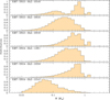 |
Fig. 8 Posteriors for the mass of the lens systems. |
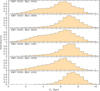 |
Fig. 9 Posteriors for the distance to the lens systems. |
Physical lens parameters.
7 Summary and conclusion
We carried out detailed analyses of six microlensing events: KMT-2023-BLG-0548, KMT-2023-BLG-0830, KMT-2023-BLG-0949, KMT-2024-BLG-1281, KMT-2024-BLG-2059, and KMT-2024-BLG-2242. These events were identified in the KMTNet survey data collected during the 2023 and 2024 observing seasons, as part of a targeted search for microlensing events exhibiting anomalies with durations shorter than one day. Such short-lived anomalies may indicate the presence of a planetary companion to the lens, prompting a detailed investigation to determine the nature and origin of the observed perturbations.
We modeled the observed light curves using various lens-system configurations that could produce short-term anomalies, including a planetary companion to the lens, a very wide or close binary lens companion, and a faint source companion. We also considered the potential for multiple interpretations due to lensing degeneracies. We found that planetary companions to the lenses are responsible for the anomalies in all analyzed events. In the case of the two events KMT-2024-BLG-2059 and KMT-2024-BLG-2242, the duration was short due to the small caustic size induced by low-mass planet. However, the short durations of anomalies in other events arose from different causes. In the case of KMT-2023-BLG-0548, the anomaly was brief due to the substantial deviation of the planetary separation from the Einstein radius, leading to a small caustic size. For KMT-2023-BLG-0830 and KMT-2024-BLG-1281, the short duration of the anomaly was caused by a combination of a small planet-to-host mass ratio and the restricted crossing area of the source, resulting from the elongated shape of the caustic. In KMT-2023-BLG-0949, the source traversed only a small portion of the caustic, which resulted in the short-lived anomaly.
We determined the physical parameters of the lens systems through Bayesian analysis, combining constraints from the observed lensing parameters with priors based on a Galactic model and the lens mass function to estimate the most probable values. For KMT-2023-BLG-0548, the Bayesian posterior shows two distinct mass peaks: the lower-mass peak suggests a sub-Jovian planet orbiting an M dwarf in the Galactic disk, while the higher-mass peak indicates a super-Jovian planet around a K-type dwarf in the bulge. For KMT-2023-BLG-0830, the lens system comprises a Neptune-mass planet orbiting an M dwarf, located in the Galactic bulge. For KMT-2023-BLG-0949, the lens system consists of a super-Jovian planet orbiting a ~0.5 M⊙ host at a distance of roughly 6 kpc. For KMT-2024-BLG-1281, the lens is consisted of a planet with a mass slightly greater than that of Neptune and and an M-dwarf host star. The planet KMT-2024-BLG-2059Lb, with a mass about seven times that of Earth, is classified as a super-Earth and orbits an M dwarf of ~0.5 M⊙. The short timescale and small angular Einstein radius of KMT-2024-BLG-2242 suggest a ~0.07 M⊙ host, likely a brown dwarf, with a planet comparable in mass to Uranus or Neptune.
Although the physical parameters of the lens in the analyzed microlensing events are subject to considerable uncertainty due to incomplete measurements of the lensing observables, these uncertainties can be significantly mitigated through future high-resolution follow-up observations. Instruments such as the Keck Adaptive Optics (AO) system on the 10-meter Keck Telescope and the upcoming 30-meter European Extremely Large Telescope (E-ELT), which is expected to become operational around 2030, will facilitate such observations. High-resolution imaging will enable the spatial resolution of the lens and source, allowing for direct confirmation of microlensing models by comparing the lens-source relative proper motion inferred from light curve modeling with that measured from follow-up data. Furthermore, resolving the lens will provide tighter constraints on the properties of the planetary host and help to break degeneracies in the estimates of lens mass and distance, particularly in cases with multiple degenerate solutions, such as KMT-2023-BLG-0548.
Among the six newly discovered planets, four are found to have masses significantly lower than that of Jupiter in our solar system. Recently, Zang et al. (2025) conducted a statistical analysis of planet-to-host mass ratios using a sample of exoplanets discovered through the KMTNet survey, revealing that planets in Jupiter-like orbits exhibit a bimodal distribution, with distinct peaks corresponding to super-Earths and gas giants. Of the low-mass planets reported in this study, KMT-2024-BLG-2059Lb falls into the super-Earth category, while the other three (KMT-2023-BLG-083Lb, KMT-2024-BLG-1281Lb, and KMT-2024-BLG-2242Lb) are comparable in mass to Uranus-like planets in our solar system. Although the Zang et al. study was based on a total of 63 planets, this sample size remains relatively limited. The newly reported planets are therefore expected to contribute meaningfully to refining the statistical analysis and improving the robustness of conclusions about the demographics of cold exoplanets.
Acknowledgements
This research has made use of the KMTNet system operated by the Korea Astronomy and Space Science Institute (KASI) at three host sites of CTIO in Chile, SAAO in South Africa, and SSO in Australia. Data transfer from the host site to KASI was supported by the Korea Research Environment Open NETwork (KREONET). C.Han acknowledge the support from the Korea Astronomy and Space Science Institute under the R&D program (Project No. 2025-1-830-05) supervised by the Ministry of Science and ICT. J.C.Y., I.G.S., and S.J.C. acknowledge support from NSF Grant No. AST-2108414. W. Zang acknowledges the support from the Harvard-Smithsonian Center for Astrophysics through the CfA Fellowship. The MOA project is supported by JSPS KAKENHI Grant Number JP16H06287, JP22H00153 and 23 KK 0060. C.R. was supported by the Research fellowship of the Alexander von Humboldt Foundation.
References
- Albrow, M. 2017, MichaelDAlbrow/pyDIA: Initial Release on Github, Version v1.0.0, https://doi.org/10.5281/zenodo.268049 [Google Scholar]
- Bennett, D. P., & Rhie, S. H. 1996, ApJ, 458, 293 [Google Scholar]
- Bensby, T., Yee, J. C., Feltzing, S., et al. 2013, A&A, 549, A147 [NASA ADS] [CrossRef] [EDP Sciences] [Google Scholar]
- Bessell, M. S., & Brett, J. M. 1988, PASP, 100, 1134 [Google Scholar]
- Bond, I. A., Abe, F., Dodd, R. J., et al. 2001, MNRAS, 327, 868 [Google Scholar]
- Chung, S.-J., Han, C., Park, B.-G., et al. 2005, ApJ, 630, 535 [Google Scholar]
- Dong, S., DePoy, D. L., Gaudi, B. S., et al. 2006, ApJ, 642, 842 [NASA ADS] [CrossRef] [Google Scholar]
- Dominik, M. 1999, A&A, 349, 108 [NASA ADS] [Google Scholar]
- Gaudi, B. S. 1998, ApJ, 506, 533 [Google Scholar]
- Gaudi, B. S., & Gould, A. 1997, ApJ, 486, 85 [Google Scholar]
- Gaudi, B. S., & Han, C. 2004, ApJ, 611, 528 [NASA ADS] [CrossRef] [Google Scholar]
- Gould, A., & Loeb, A. 1992, ApJ, 396, 104 [Google Scholar]
- Gould, A., Han, C., Zang, W., et al. 2022, A&A, 664, A13 [NASA ADS] [CrossRef] [EDP Sciences] [Google Scholar]
- Griest, K., & Safizadeh, N. 1998, ApJ, 500, 37 [Google Scholar]
- Han, C. 2006, ApJ, 638, 1080 [Google Scholar]
- Han, C., & Gaudi, B. S. 2008, ApJ, 689, 5 [Google Scholar]
- Han, C., Udalski, A., Jung, Y. K. 2023, A&A, 670, A172 [NASA ADS] [CrossRef] [EDP Sciences] [Google Scholar]
- Han, C., Bond, I. A., Lee, C.-U., et al. 2024a, A&A, 687, A225 [NASA ADS] [CrossRef] [EDP Sciences] [Google Scholar]
- Han, C., Albrow, M. D., Lee, C.-U., et al. 2024b, A&A, 689, A209 [NASA ADS] [CrossRef] [EDP Sciences] [Google Scholar]
- Han, C., Ryu, Y., Lee, C.-U., et al. 2024c, A&A, 692, A106 [NASA ADS] [CrossRef] [EDP Sciences] [Google Scholar]
- Han, C., Bond, I. A., Jung, Y. K., et al. 2025, A&A, 694, A90 [NASA ADS] [CrossRef] [EDP Sciences] [Google Scholar]
- Hwang, K.-H., Choi, J.-Y., Bond, I. A., et al. 2013, ApJ, 778, 55 [Google Scholar]
- Hwang, K.-H., Zang, W., Gould, A., et al. 2022, AJ, 163, 43 [NASA ADS] [CrossRef] [Google Scholar]
- Jung, Y. K., Han, C., Udalski, A., et al. 2021, AJ, 161, 293 [NASA ADS] [CrossRef] [Google Scholar]
- Jung, Y. K., Zang, W., Han, C., et al. 2022, AJ, 164, 262 [NASA ADS] [CrossRef] [Google Scholar]
- Kervella, P., Thévenin, F., Di Folco, E., & Ségransan, D. 2004, A&A, 426, 29 [Google Scholar]
- Kim, S.-L., Lee, C.-U., Park, B.-G., et al. 2016, JKAS, 49, 37 [Google Scholar]
- Kim, D.-J., Kim, H.-W., Hwang, K.-H., et al. 2018, AJ, 155, 76 [Google Scholar]
- Mao, S., & Paczyński, B. 1991, ApJ, 374, 37 [Google Scholar]
- Nataf, D. M., Gould, A., Fouqué, P. et al. 2013, ApJ, 769, 88 [Google Scholar]
- Sumi, T., Abe, F., Bond, I. A., et al. 2003, ApJ, 591, 204 [NASA ADS] [CrossRef] [Google Scholar]
- Udalski, A., Szymański, M. K., & Szymański, G. 2015, Acta Astron., 65, 1 [NASA ADS] [Google Scholar]
- Yang, H., Yee, J. C., Hwang, K.-H., et al. 2024, MNRAS, 528, 11 [NASA ADS] [CrossRef] [Google Scholar]
- Yee, J. C., Shvartzvald, Y., Gal-Yam, A., et al. 2012, ApJ, 755, 102 [Google Scholar]
- Yee, J. C., Zang, W., Udalski, A., et al. 2021, AJ, 162, 180 [NASA ADS] [CrossRef] [Google Scholar]
- Yoo, J., DePoy, D. L., Gal-Yam, A., et al. 2004, ApJ, 603, 13 [Google Scholar]
- Zhai, R., Poleski, R., Zang, W., et al. 2024, AJ, 167, 162 [NASA ADS] [CrossRef] [Google Scholar]
- Zang, W., Hwang, K.-H., Udalski, A., et al. 2021, AJ, 162, 163 [NASA ADS] [CrossRef] [Google Scholar]
- Zang, W., Jung, Y. K., Yee, J. C., et al. 2025, Science, 388, 400 [Google Scholar]
- Zhang, K., Gaudi, B. S., & Bloom, J. S. 2022, Nat. Ast. 6, 782Z [Google Scholar]
All Tables
All Figures
|
Fig. 1 Light curve of the microlensing event KMT-2023-BLG-0548. The bottom panel displays the full light curve, while the upper panels present a zoomed-in view of the peak region along with the residuals for four different models. The four insets in the bottom panel illustrate the lens-system configurations corresponding to the four degenerate 2L1S solutions. In each inset, the closed figure composed of concave curves represents the caustics, and the arrowed line indicates the source trajectory. The orange circle, scaled to represent the angular size of the source, on the trajectory marks the source’s position at the moment of peak anomaly. |
| In the text | |
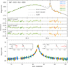 |
Fig. 2 Lensing light curve of KMT-2023-BLG-0830. The notations are consistent with those in Fig. 1. |
| In the text | |
|
Fig. 3 Light curve of KMT-2023-BLG-0949. We note that in addition to the strong anomaly near the peak, there are also additional weak extended negative deviations in the rising part of the light curve. |
| In the text | |
|
Fig. 4 Light curve of the lensing event KMT-2024-BLG-1281. |
| In the text | |
|
Fig. 5 Lensing light curve of the event KMT-2024-BLG-2059. |
| In the text | |
|
Fig. 6 Lensing light curve of KMT-2024-BLG-2242. |
| In the text | |
|
Fig. 7 Locations of source stars (blue dots) with respect to the centroid of the red giant clump (RGC, red dots) in the instrumental color-magnitude diagrams of the six planetary lensing events. For events with measured blended flux, the positions of the blend (green dots) are also indicated. |
| In the text | |
|
Fig. 8 Posteriors for the mass of the lens systems. |
| In the text | |
|
Fig. 9 Posteriors for the distance to the lens systems. |
| In the text | |
Current usage metrics show cumulative count of Article Views (full-text article views including HTML views, PDF and ePub downloads, according to the available data) and Abstracts Views on Vision4Press platform.
Data correspond to usage on the plateform after 2015. The current usage metrics is available 48-96 hours after online publication and is updated daily on week days.
Initial download of the metrics may take a while.