| Issue |
A&A
Volume 702, October 2025
|
|
|---|---|---|
| Article Number | A26 | |
| Number of page(s) | 20 | |
| Section | Galactic structure, stellar clusters and populations | |
| DOI | https://doi.org/10.1051/0004-6361/202554938 | |
| Published online | 02 October 2025 | |
DAWN
I. Simulating the formation and early evolution of stellar clusters with Phantom N-Body
1
Univ. Grenoble Alpes, CNRS, IPAG,
38000
Grenoble,
France
2
School of Physics and Astronomy, Monash University,
Vic. 3800,
Australia
★ Corresponding author.
Received:
1
April
2025
Accepted:
4
August
2025
Abstract
Context. The star formation process produces hierarchical clustered stellar distributions through gravoturbulent fragmentation of molecular clouds. Simulating stellar dynamics in such an environment is numerically challenging due to the strong coupling between young stars and their surrounding and the large range of length and time scales.
Aims. This paper is the first of a suite aimed at investigating the complex early stellar dynamics in star-forming regions, from the initial collapse of the molecular cloud to the phases of complete gas removal. We present a new simulation framework. This advanced framework is the key to generating a larger set of simulations, enabling statistical analysis, which is mandatory to address the stochastic nature of dynamical interactions.
Methods. Methods originating from the stellar dynamics community, including regularisation and slow-down methods (SDAR), have been added to the hydrodynamical code Phantom to produce simulations of embedded cluster early dynamics. This is completed by a novel prescription of star formation to initialise stars with a low numerical cost, but in a way that is consistent with the gas distribution during the cloud collapse. Finally, a prescription for H II region expansion has been added to model the gas removal.
Results. We have run test-case simulations following the dynamical evolution of stellar clusters from the cloud collapse to a few million years. Our new numerical methods fulfil their function by speeding up the calculation. The N-body dynamics with our novel implementation never appear as a bottleneck that stalls the simulation before its completion. Our new star formation prescription avoids the need to sample individual star formations within the simulated molecular clouds with high resolution. Overall, these new developments allow accurate hybrid simulations in minimal calculation time. Our first simulations show that massive stars largely impact the star formation process and shape the dynamics of the resulting cluster. Depending on the position of these massive stars and the strength of their H II regions, they can prematurely dismantle part of the cloud or trigger a second event of cloud collapse, preferentially forming low-mass stars. This leads to different stellar distributions for numerical simulations with similar initial conditions and confirms the need for statistical studies. Quantitatively, and despite the implementation of feedback effects, the final star formation efficiencies are too high compared with those measured in molecular clouds of the Milky Way. This is probably due to the lack of feedback mechanisms other than H II regions, in particular jets, non-ionising radiation, or Galactic shear.
Conclusions. Our new Phantom N-Body framework, coupled with the novel prescription of star formation, enables the efficient simulation of the formation and evolution of star clusters. It enables the statistical analysis needed to establish a solid theoretical framework for the dynamical evolution of embedded star clusters, continuing the work done in the stellar dynamics community.
Key words: gravitation / hydrodynamics / methods: numerical / stars: formation / stars: kinematics and dynamics / open clusters and associations: general
© The Authors 2025
 Open Access article, published by EDP Sciences, under the terms of the Creative Commons Attribution License (https://creativecommons.org/licenses/by/4.0), which permits unrestricted use, distribution, and reproduction in any medium, provided the original work is properly cited.
This article is published in open access under the Subscribe to Open model. This email address is being protected from spambots. You need JavaScript enabled to view it. to support open access publication.
1 Introduction
Star formation occurs within turbulent, collapsing molecular clouds in the Galaxy. The gravitational collapse of these turbulent clouds produces interconnected filaments and hubs that amplify density anisotropies. Observations with the Spitzer telescope have revealed that the star formation process takes place preferentially inside these dense structures in star-forming regions (Evans et al. 2009; Gutermuth et al. 2009; André et al. 2014). Denser regions with similar levels of turbulent and magnetic support are more sensitive to fragmentation, leading to a dominant ‘clustered’ star formation channel. Consequently, the distribution of newborn stars is inherited from the distribution of filaments, hubs and ridges (Schneider et al. 2010; Peretto et al. 2013; Motte et al. 2018), and appears to be structured, with multiple clusters embedded in their birth nebula.
Observations have shown that this clustered state is transient for 90% of stars (Lada & Lada 2003), and that only 10% of newborn stars remain in open clusters after 10 Myr. This dynamical evolution is fast and complex, and a better understanding of this evolution is needed to constrain environmental properties required in other fields. For example, the statistics of fly-by events during the early evolution of star-forming regions could help to constrain their effect on planet formation within protoplanetary discs (Cuello et al. 2023).
Pure N-body simulations (Aarseth & Hills 1972; Goodwin & Whitworth 2004; Bastian & Goodwin 2006; Parker et al. 2014; Wright et al. 2014) have tried to explain the rapid dissolution of natal star clusters with stellar dynamics. These simulations model young stellar clusters using an initially fractal spatial distribution, consistent with observational constraints (Cartwright & Whitworth 2004). The results indicate that dynamical instabilities, such as close encounters or unstable triples, can lead to the complete dissolution of an initial cluster or to the conservation of a strongly bound cluster of stars at the end of the simulation. Furthermore, the statistical robustness of these findings is ensured by the averaging of hundreds of simulations to draw conclusions. However, pure N-body simulations ignore one key component of this dynamical evolution: the strong links and interactions between newborn stars and their gaseous environment. Previous N-body studies have attempted to account for the gas potential using simple radial analytical formulae with a decay in time to model the gas expelled from embedded clusters (Kroupa et al. 2001). More recent simulations focus on the early phases of star formation, revealing the complex and time-variable nature of this coupling that influences both the dynamics and the formation of stars. (Verliat et al. 2022; Fujii et al. 2021; Grudić et al. 2021; González-Samaniego & Vazquez-Semadeni 2020). Hence, only direct methods can model star formation and stellar feedback simultaneously to follow the stellar dynamics during the early evolution of clusters in star-forming regions.
On the other hand, numerical studies focusing on star formation have naturally characterised this process using a direct hydrodynamic model. Larson (1969) and Boss & Bodenheimer (1979) focused on a single, isolated clump of gas gravitationally collapsing to form single or binary stars. Such works tried to self-consistently follow the collapse from the initial dense clump up to the onset of nuclear fusion (Bate 1998; Bate et al. 2014; Wurster et al. 2018). Recent studies (e.g. Ahmad et al. 2024; Mauxion et al. 2024) continue to refine models of protostar formation, incorporating more realistic physical processes to predict phenomena such as the formation and evolution of protoplanetary discs that are essential to planet formation.
However, the star formation community rapidly understood that the environment is key to explaining stellar properties. Hence, it became critical to perform simulations at the molecular cloud scale while modelling the formation of individual protostars. Bate et al. (1995) developed a method called sink particles that hides dense parts of a collapsing clump inside a massive particle capable of accreting infalling material without computationally expensive hydrodynamic calculations. This method unlocked the ability to follow the evolution of star-forming regions beyond the point of initial collapse. As a consequence, sink particles are now used in almost every star formation simulation.
Early studies (Bate et al. 2002; Bate & Bonnell 2005) simulated small, isolated molecular clouds with a diameter of a fraction of a parsec and an initial mass of tens of solar masses. Later developments enabled the modelling of radiative feedback from protostars on the surrounding gas, which was found to be essential to produce a more convincing stellar mass distribution (e.g. Bate 2009; Hennebelle et al. 2020). Other studies identify links between initial molecular cloud conditions, such as the temperature, magnetic field (Myers et al. 2014; Lee & Hennebelle 2019), or initial turbulent state (Joos et al. 2013; Liptai et al. 2017), and stellar properties such as the mass or the spatial distribution. Most recent studies attempt to model physical processes in star-forming regions more realistically. Specifically, stellar feedback is thought to play a major role in both star formation and the global evolution of molecular clouds (Krumholz et al. 2014). Verliat et al. (2022) find that protostellar jets can regulate accretion around dense objects by injecting turbulent support inside the surrounding gas. State-of-the-art simulations attempt to model the evolution of giant molecular clouds through the entire star formation process, from the initial collapse to the gas removal mainly driven by H II region expansion produced by massive stars (Guszejnov et al. 2022). For instance, Wall et al. (2019) and Fujii et al. (2022) reuse methods from the stellar dynamics community in their hydrodynamic codes to perform what is called a hybrid hydro/N-body simulation.
These simulations aim to bridge the gap between previous work by the stellar dynamics community and star cluster formation simulations, including stellar feedback. They provide a framework to explain the dynamical evolution of young star clusters influenced by their environment. However, they do not follow the statistical approach of previous pure N-body cluster simulations, which is needed to identify typical evolutionary tracks followed during the stochastic dynamics of stars in a cluster.
In this paper, we showed how methods developed for accelerating N-body simulations and efficient star formation and stellar feedback prescriptions can be incorporated directly into a 3D hydrodynamics code, adding missing physics to pure N-body simulations. Such a framework allowed us to initialise young embedded clusters directly from star formation in a molecular cloud collapse, leading to self-consistent cluster initial conditions linked with the natal gaseous environment. Their evolution can therefore be followed through the direct influence of the gas, itself influenced by gravity and stellar feedback. We aim to follow this evolution up to the emergence of clusters from their natal cloud. Our new framework has been designed to be fast enough to enable the statistical approach necessary to study the dynamical evolution of embedded clusters.
The paper is organised as follows. First, N-body algorithms newly implemented in the code Phantom (Price et al. 2018) are presented in Sect. 2. Section 3 describes the new star formation prescription (Sect. 3.1), the implementation of H II region feedback (Sect. 3.2), and the fiducial model studied in this work (Sect. 3.3). Simulation results of this model are described and discussed in Sect. 4. Section 5 discusses numerical performance and accuracy. Finally, Section 6 gives our conclusions and summarises future prospects. Paper II will then be dedicated to a deeper investigation of our new star formation prescription, focusing on the mass distribution and multiplicity statistics.
2 Phantom
and N-body algorithms Simulations presented in this work were performed with the 3D smoothed particle magnetohydrodynamics (SPMHD) code Phantom (Price et al. 2018). Smoothed particle hydrodynamics (SPH; Lucy 1977; Gingold & Monaghan 1977) solvers use a Lagrangian approach to solve fluid equations by discretising the medium into particles of fixed mass that follow the fluid motion. Fluid forces are derived by calculating quantities on these particles with neighbour-weighted sums using smoothing kernels (Price 2012). We chose Phantom because of its versatility. It is capable of modelling a variety of astrophysical systems with its numerous physics modules, such as a magnetohydrodynamics solver (ideal and non-ideal), self-gravity, dust, chemical networks, sink particles, and more. However, this code was not yet ready to perform embedded cluster simulations at the beginning of this work. While a few studies on star formation have already been carried out (Liptai et al. 2017; Wurster & Bonnell 2023), these studies stop the evolution of their star-forming region at around the initial freefall time of the cloud, τff. This end time is limited by the large computational cost of such models. One of the growing constraints is the gravitational dynamics between newly formed stars when no softening is applied, which can then form in close binaries or multiple systems. Stars in such systems are subject to strong interactions that result in small time-step constraints that can dramatically slow down a simulation.
In Phantom, gravitational forces between point masses (as stars) are computed using a direct method. This direct algorithm is coupled to a Leapfrog symplectic integrator to follow the dynamics of stars. This integrator is only second order, and needs short time steps to reach a sufficient accuracy. This combination of methods is inefficient and can be inaccurate during the early evolution of embedded clusters. As the number of steps to integrate a cluster up to a few million years is prohibitive, it also implies an accumulation of truncation errors that can drastically change the evolution of close binaries or multiples, which are key in the overall cluster evolution. A hard binary disruption due to inaccuracy in the integration scheme can lead to the artificial fast expansion of the host cluster. These numerical effects motivated new implementations written in Phantom that reuse methods developed in collisional N-body codes, the slow-down algorithmic regularisation (SDAR) method proposed by Wang et al. (2020b), and the forward symplectic integrator (FSI) recently presented in Rantala et al. (2021) and Dehnen & Hernandez (2017). For the sake of completeness, we described our implementation from these original papers in Appendix A.1.
2.1 Forward symplectic integrator: FSI
Symplectic integrators preserve conservation properties. They can conserve angular momentum to round-off error while constraining the energy error inside a small range, depending on the truncation order and the time-step choice. They achieve that by rewriting the time evolution operator. This new formulation implies that the integrated Hamiltonian is slightly different from the true one by what is called the error Hamiltonian. The art of building high-order symplectic integrators lies in minimising this error term (Yoshida 1990). The FSI (Dehnen & Hernandez 2017; Rantala et al. 2021) achieves this minimisation up to the fourth order with the unique property of producing no backward substeps inside its scheme, which is essential if dissipative forces are in the scheme. More details on how to construct symplectic integrators are presented in Appendix A.1. That aside, the new time evolution operator derived from this special method is written as
 (1)
(1)
where H is the Hamiltonian, T the kinetic energy, U the potential, and G an extra potential. All the coefficients in this time evolution operator are strictly positive. The middle operation is modified with what is commonly called a gradient force evaluation produced by a slightly different potential,  (cf., Rantala et al. 2021). Knowing the definition of G and for a system composed only of N point masses coupled by gravitational interactions, where aj is the acceleration sensed by each mass, the gradient acceleration can be written as
 (2)
(2)
Expanding the partial derivative in this equation leads to the common formula of the jerk computed in Hermite fourth-order integrator (Makino & Aarseth 1992) and gives
![Mathematical equation: ${g_i} = 2\mathop \sum \limits_{i = 1}^N \mathop \sum \limits_{i \ne j}^N {{G{m_j}} \over {{r_{ij}}}}\left[ {r_{ij}^2{a_{ij}} - 3\left( {{r_{ij}} \cdot {a_{ij}}} \right){r_{ij}}} \right],$](/articles/aa/full_html/2025/10/aa54938-25/aa54938-25-eq4.png) (3)
(3)
where aij and rij are the relative acceleration and position between particles i and j. The modified acceleration of the middle kick operation for a particle, i, is then
 (4)
(4)
This formula is not trivial to compute. First, all pairwise accelerations are required to compute each gradient term, which means that they need to be evaluated beforehand. During the middle kick phase, there is therefore one acceleration and one gradient acceleration evaluation consecutively to compute the final acceleration to kick the velocity of each body in the system. This method turned out to be expensive to implement in the current Phantom framework. Indeed, gradient accelerations in a simulation where softening is applied between stars and gas need to take this softening into account, which is possible but numerically complex. Instead, Omelyan (2006) proposed computing this modified acceleration by extrapolating it from a slightly shifted position of each body, which depends on the standard acceleration. Formally, it is written as
 (5)
(5)
and a is the function to compute the acceleration for each particle in the system. One can see in this formula that there are still two acceleration evaluations. However, it reuses the same function in both cases, with a shifted position in the latter one. Omelyan (2006) and Chin & Chen (2005) showed that this new formula gives results close to the original. This method is far easier to implement in an existing framework. Hence, we chose this method instead of the original one.
In terms of precision, FSI outperforms all other standard fourth-order symplectic schemes such as the Forest-Ruth integrator (Forest & Ruth 1990) and even improved ones such as the Position extended Forest-Ruth-like integrator (PEFRL)(Omelyan et al. 2002) (see Appendix A.1). Chin & Chen (2005) argued that even with the same order of truncation error, the forward scheme will always outperform standard schemes because others evaluate forces far from the true trajectory of the object. By contrast, forward schemes evaluate forces very close to the true trajectory with the same time step resolution. In the end, standard schemes need smaller time steps to achieve the same resolution. FSI seemed to be the best option for a new integration algorithm of point masses in Phantom. It has one of the best precisions for fourth-order schemes with limited supplementary force evaluation in one global step. Its forward nature assures that nothing can go wrong if dissipation is present in the system, which is often the case in astrophysical hydrodynamical simulations.
2.2 Slow-down algorithmic regularisation: SDAR
2.2.1 Regularised integration
The FSI presented above is an accurate integrator that already outperforms second-order leapfrog schemes. It is then possible to limit the number of steps per orbit needed to sample a good trajectory of each body. Typically, this number of sample points is set from 300 to 500 with the previous Leapfrog integrator. With the new FSI, we were able to easily divide this number by a factor of four while retaining better accuracy.
However, updating the main integrator was not enough to resolve the stellar dynamics within an embedded cluster in a reasonable computation time. Stellar densities are high in cluster environments, and binaries and multiple systems represent a significant fraction of the population (Offner et al. 2023). These systems can produce strong computational constraints during close encounters or with short-period binaries. For example, a binary with 10 au separation and a total mass of 2 M⊙ has a period around 20 yr. It could then produce a time step constraint around δt = 0.33 yr when the typical freefall time of a molecular cloud in this study is around 5.5 Myr, which gives a large dynamic range. This simple example does not capture the stringent time step constraints that could appear in a young cluster. Day orbit period binaries and high eccentric ones make direct computation infeasible.
The stellar dynamics community has already tackled these high dynamical scale problems to model the long-term evolution of stellar clusters containing a few thousand bodies to a few tenths of a million. To meet this challenge, sophisticated methods have been developed to manage the two main issues at large dynamic ranges, which are the gravitational singularity during pair interaction and the secular evolution of multiple systems.
First, gravitational pair interaction is a function of the inverse square distance between two bodies. It produces a singularity at the distance d = 0. This singularity can strongly constrain the simulation time step. During close encounters or periapsis approaches in a highly eccentric binary, the velocity of the two bodies can dramatically increase due to the inverse square distance proportionality of their interactions. Their true trajectory will be missed if there are not enough sample points. Worse, the pair interaction can produce false runaway bodies. In collisionless models as cosmological ones such as Gadget 4 (Springel et al. 2021), the interaction is softened in a certain radius around each point mass to avoid these strong pair interactions. However, softening methods are prohibited in collisional N-body codes, as the collisional dynamics govern the future evolution of a cluster. The immediate solution could be to increase the number of steps. However, this would also produce large truncation and roundoff errors due to the accumulation of steps, in addition to being computationally expensive.
Various methods have been proposed in the literature for 50 years now (Kustaanheimo et al. 1965; Mikkola & Aarseth 2002) to manage these two issues. All of them are based on the same idea: regularisation of gravitational interactions. The idea is to hide the singularity. One manipulates the equations of motion by applying spatial and time transformations to the system of equations to make the 1/d2 term in the force evaluation vanish. The first regularisation method used in this field was proposed by Kustaanheimo et al. (1965) (KS method). It transforms binary gravitational motion into a simple harmonic oscillator, meaning that the time step can be constant during a whole period of the binary, whatever its eccentricity. The details of this transformation can be found in the original paper and in Aarseth (2003). It has been successfully used in several collisional codes in the past, such as the series of Aarseth’s N-Body codes (Aarseth 1999). However, its complexity made it hard to implement. In addition, KS regularisation of multiple systems requires specialised methods, which add up to a rather complex method. More recent codes (Wang et al. 2020a; Rantala et al. 2023) preferred a different approach to reach the same results, using what is called an ‘algorithmic regularisation’ (AR) (Mikkola & Tanikawa 1999; Preto & Tremaine 1999). This work followed the same approach. AR methods apply a time transformation to the system,
 (6)
(6)
where s is a new time integration variable that is linked with the real time, t, by a time transformation function, Ω(r). This function is often taken as the gravitational potential of the system.
In contrast to KS, it leaves the spatial co-ordinates unchanged. The singularity is still present in a pair interaction. However, the idea is then to use a specialised algorithm to produce regular results. There are two main algorithms to achieve that. The LogH method presented in Rantala etal. (2023) or Aarseth (2003) and the time-transformed leapfrog (TTL) (Mikkola & Aarseth 2002). We adopted the latter method in this work, which is described in detail in Appendix A.2. Briefly, it is possible to construct a new symplectic integrator using the modified system of equations. The change of variable produces a new integrated momentum-like variable, W, defined as
 (7)
(7)
This new variable will then have the same behaviour as velocities in a symplectic scheme. The Leapfrog method that lends its name to this method is not precise enough in such applications. Two solutions have been used to reach a satisfactory accuracy. First, the original algorithm from Mikkola’s code and the new code BIFROST (Rantala et al. 2023) used the Gragg–Bulirsch–Stoer (GBS) extrapolation method (Gragg 1965; Bulirsch & Stoer 1966) to ensure a user-chosen relative error. The second solution used in PeTar (Wang et al. 2020a), another stellar dynamics code, is to integrate the system with a high-order symplectic scheme from Yoshida (1990). We chose the latter method for its simplicity. However, GBS extrapolation will be tested in further work.
The essence of this method can be understood from the time transformation (Eq. (6)). The link between the new integration variable, s, and the real time, t, depends on the potential strength. This way, s can have constant large time steps as the integrated time, t, will scale depending on the potential strength. It means that when the gravitational forces are strong (close to the singularity), the time integration will be slow and algorith-mically adjusted to the potential strength. That way, singularity approaches are not an issue anymore even if it is still present in equations.
2.2.2 Slowed down binaries
The last challenge to tackle is the secular evolution of perturbed binaries and multiple systems. Regularised integrators can solve collisional trajectory issues. Nevertheless, they still need a few sample points to integrate orbits. It means that very hard, eccentric, and weakly perturbed binaries or stable triple systems can bottleneck the computation, as the dynamic time range between a cluster and these systems can be extremely large. Because of their hardness, these binaries can be considered unperturbed, and thus their motion can be found analytically using Kepler solvers. It resolves only a part of the issue, as stable triples are commonly found in simulations and close encounters in dense stellar regions can greatly perturb binary systems. Mikkola & Aarseth (1996) proposed a solution with the cost of losing the orbital phase of these hard binaries. The slow-down method proposes to slightly modify the original Hamiltonian of a weakly perturbed binary according to
 (8)
(8)
where κ is called the slow-down factor and Hb is the unperturbed binary Hamiltonian. This equation means that only the binary dynamics are scaled down by a factor, κ. Original velocities are conserved by this scaling. Equations of motion derived from this Hamiltonian are given by
 (9)
(9)
 (10)
(10)
where U is an arbitrary external potential and i and c index points on one binary member and its companion, respectively. One can see that the forces due to gravitational interactions between the primary and the secondary are scaled down by κ. The original orbital period of the binary is divided by κ. It is then straightforward to understand that the time constraint on the binary will be relaxed by the same factor.
Equations (9) and (10) show that for a given binary system, its orbital parameters are conserved by the scheme, despite perturbations that will be discussed shortly. It also means that even if the apparent period is κ times longer than the original one, the true orbital parameters are conserved by the scheme. The only change comes from the external perturbation.
Wang et al. (2020b) showed that applying this method to one slow-down period, Psd = κΡ, gives the same velocity modification as if the system was integrated during κΡ. This means that the slow-down method averages perturbations applied to the binary on a slow-down period, Psd. Nonetheless, it is only applicable if the perturbation is weak enough. Thus, it means that κ should be chosen carefully to preserve the accuracy of the averaging. On intermediate perturbed binaries, this averaging property is relevant only for a few orbits. By contrast, external perturbations can be almost negligible for a hard binary. In that case, the averaging property can be accurate enough on several orders of magnitude of the original orbital period.
The generalisation to a few-body problem is straightforward and detailed in Wang et al. (2020b). Only two changes are needed: i) the bulk motion of a whole binary in an N-body system is not slowed down and ii) the perturbation on a binary of the system is now the summation of each direct gravitational force produced by each perturber inside the system. As shown above, κ quantifies the number of original periods where the perturbation applied to the binary can be averaged. On a highly perturbed binary, it is impossible to average the perturbation on multiple periods, which means κ = 1. A hard binary can stay unperturbed during a whole simulation. The averaging is not risky at all, and then κ can stay at a high value. However, one can see that this factor needs to scale with the strength of the perturbation. A special method has been added to our implementation to modulate κ depending on external perturbations following Mikkola & Aarseth (1996). A detailed overview is presented in Appendix A.3, and a unit test performed to validate the implementation is presented in Appendix C.
The slow-down method can easily be mixed up with AR, which then gives what is called a SDAR integration method (Wang et al. 2020b). This method gives an efficient integrator for multiple systems, which are common in young stellar clusters. It can be used in combination with standard integrators such as the FSI presented above to form a complete stellar dynamics framework capable of evolving an entire cluster of stars for a long time.
2.3 Phantom new N-body implementation
We implemented the integration methods described above into the public version of Phantom. They could not fit directly into the main integration routine without a major refactor. Importantly, the SDAR method is used to integrate the motion of stars but not SPH gas particles. Thus, the new methods are applied to a specific part of the system and not the entire one.
The original Phantom integration scheme is derived from the reference system propagator algorithms (Tuckerman et al. 1992) that split forces applied to particles in the system into two categories: ‘slow’ and ‘fast’ forces with, respectively, weak and strong time step constraints. This splitting allows for the construction of a two-level leapfrog scheme according to
 (11)
(11)
 (12)
(12)
 (13)
(13)
 (14)
(14)
where asph corresponds to SPH accelerations (pressure, viscosity, self-gravity, and so on). Δtsph is the time step associated with them and used in the first leapfrog level. The drift phase of the first-level leapfrog is replaced by multiple substeps of another leapfrog in association with a smaller time step, Δtfast. This subtime step is controlled by faster accelerations contained in afast, such as external potential, sink-gas, and sink-sink accelerations.
The methods we presented above relate to stars, which correspond to point masses in Phantom (sink particles without softening). This means that only the second level needs to be updated, as it is where sink particles are updated during integration. The first upgrade was to switch the coarse Leapfrog integrator for the more accurate FSI presented above. The substep integrator can then be rewritten as
 (15)
(15)
 (16)
(16)
 (17)
(17)
 (18)
(18)
 (19)
(19)
 (20)
(20)
 (21)
(21)
where ãfast is the extrapolated gradient acceleration needed to properly cancel second-order error terms in the FSI. We computed this gradient acceleration by evaluating forces twice in a row with a slightly shifted position during the second evaluation.
The SDAR method is not meant to integrate the motion of an entire cluster. It specialises in few-body evolution. Detection of subgroups of close stars is therefore mandatory to apply the SDAR method only to small groups. Gas particles are excluded from such integration methods as their gravitational softening and hydrodynamic forces can introduce unexpected behaviours in the integration. The group finding algorithm is directly derived from the one proposed in Rantala et al. (2023). Star neighbours are identified by searching them within a fixed searching radius, rneigh, around each star. The typical value used in this work was equal to 0.001 pc. A special criterion allows distant fly-by stars to enter a group if they enter the searching radius, rneigh, at the next step. It gives
 (22)
(22)
where r and υ are the relative position and velocity between the two stars tested, and C is a safety factor usually set to 0.1. This neighbour search is then used to construct the adjacency matrix of the entire system of stars in the simulation. Subgroups are then identified by searching connected components associated with this matrix using a depth-first search algorithm. On-the-fly binary detection is applied to each newly formed subgroup, which is essential for the slow-down method. This identification is done every substep to update subgroups as the system evolves.
Subgroups can then be integrated with SDAR methods separately from the entire system during the FSI drift phase. However, as explained in Rantala et al. (2023), each star in the subgroup still receives perturbations from its environment (from gas and point masses in Phantom) during the FSI kick phase. It then gives the full new integration scheme in Phantom given by
 (23)
(23)
 (24)
(24)
 (25)
(25)
 (26)
(26)
As the original Phantom integration scheme, the first integration level uses an individual time step scheme. However, the substep integration sticks with a global time step, Δtfast, chosen to be the most stringent constraint induced by fast forces. Subgroups only evolve during the SDAR phase and are excluded from the standard FSI drift routine. The SDAR integration routine uses the TTL regularisation method in association with a sixth- or eighth-order Leapfrog scheme derived from Yoshida (1990) following Wang et al. (2020b). On top of that, a slow-down is applied to binaries inside subgroups. For a group composed of only one binary, the slow-down factor, κ, is computed using outside perturbations and is constant during the whole SDAR integration. For multiple system groups, κ is computed with outside perturbations and perturbations induced by other members of the group. This κ needs to be updated at each SDAR step as inside perturbations evolve following the group dynamics. A correction of the new variable, W, introduced in the TTL needs to be applied at each kappa update to conserve all system properties. This correction has the form
 (27)
(27)
where Ω is the gravitational energy of the subgroup.
3 Physical models
3.1 Star formation prescription
In order to save computational time and enable the statistical analysis of the evolution of embedded clusters, we did not follow the molecular cloud collapse all the way to the formation of stars. Instead, we adopted a low numerical resolution and used a star formation scheme below this scale. This section provides a detailed description of this model.
3.1.1 Sink particles and resolution criteria
The star formation scheme is based on dynamic sink particle creation, already implemented in Phantom. It uses the criteria proposed in Bate et al. (1995). Collapsing clumps that reach a user-defined threshold density, ρc, will be eligible to pass a series of tests to verify that this clump will indeed quickly collapse. For example, a clump needs to be at least in marginal virial equilibrium. Formally, this gives
 (28)
(28)
where αj and βrot are the ratios of thermal and rotational energy over the gravitational energy of the clump, respectively. If the tests pass, the clump is then directly accreted onto a massive particle called a sink particle created at the centre of mass of the clump. The sink particle has an associated volume defined by a user-chosen accretion radius, racc, within which gas particles are directly accreted.
An essential point that has long been debated in the literature (Bate & Burkert 1997; Bate et al. 2002; Hubber et al. 2006) is the choice of this accretion radius together with the critical density value. The latter is typically chosen to resolve the initial Jeans mass of the clump to avoid numerical artefacts that could artificially fragment the collapsing clump. Thus, the maximal ρc and minimal racc are linked and depend on the mass resolution of the simulation. Following Hubber et al. (2006), this link is expressed as
 (29)
(29)
where Nneigh is the constant number of neighbours of a particle in an adaptive smoothing length framework (around 60 in Phantom) and m is the mass of one SPH particle. Therefore, the quantity Nneighm gives the minimum mass contained in an SPH kernel surrounding one particle, thereby corresponding to the minimum resolved clump mass in the simulation. As was mentioned above, a clump that can turn into a sink needs to be resolved, i.e. Mclump = Mjeans, min. Using Equation (29) and the expression of the Jeans length,
 (30)
(30)
one can find the maximum critical density,
 (31)
(31)
This maximum value can then be used to find the minimum accretion radius. Eq. (29) can be rewritten using the Jeans length as
 (32)
(32)
where h is the smoothing length. Here, the number 4 is derived from the size of the SPH kernel support, which is equal to 2 for the default cubic spline kernel in Phantom. The minimal accretion radius, racc, min, linked with  can then be expressed as
 (33)
(33)
Sink particles are often used to model one single star in formation (Bate et al. 2002; Lee & Hennebelle 2018), which implies resolving the opacity limit for fragmentation around a few Jupiter masses (Low & Lynden-Bell 1976). This can only be done for relatively small initial molecular clouds to keep the computational time reasonable. For example, the initial mass of the cloud in Bate & Bonnell (2005) was set to 50 M⊙ using 3.5 million SPH particles, allowing them to resolve the minimum Jeans mass in their simulations (0.0011 M⊙) with about 80 SPH particles. The sink particle accretion radius was correspondingly set to 5 au, which is the typical size of the first Larson core (Larson 1969). It ensures that only one star will form in a sink. Following star formation down to this scale within an entire giant molecular cloud would require a tremendous number of SPH particles and is currently beyond the reach of CPU-based codes such as Phantom.
Other methods have been proposed to describe star formation within GMC following what was done in galaxy-scale simulations (Renaud et al. 2017). In these simulations, sink particles are sufficiently large to represent small clusters of stars that form together in the same volume. A similar approach recently developed in Wall et al. (2019) considers sink particles as a stellar forge that produces stars from a list of masses sampled at the birth of each sink. As gas accretes onto these sinks, stars are generated at sink positions following the list of masses. Liow et al. (2022) proposed to group several sinks on the same list to produce more massive stars that cannot be generated by just one.
However, these methods introduce unwanted behaviour. For example, when stars are generated in a sink, the sink remains in the simulation with almost no mass in its reservoir. When accretion restarts, the sink position and velocity are mass-averaged with new accreted gas. As the sink mass is near zero, its position jumps to the accreted gas position. Due to the number of stars generated, sink particles in these simulations exhibited artificial Brownian-like motions. The erratic motion of these sinks can completely change the gas infall geometry and then perturb the spatial distribution of stars in the cluster.
3.1.2 New star formation prescription from sink particles
We proposed a new prescription to model star formation using ‘large’ sink particles where the fragmentation and accretion processes are not yet over. Typically, accretion radii are set to a few thousand astronomical units in this prescription. In that sense, sinks can be compared to the dense cores observed in star-forming regions.
However, these sinks are not necessarily cores from an observational point of view. They start their life as collapsing or marginally stable clumps. However, their future evolution is based on the sub-sink scale physics that will be described in the following. This evolution can diverge from what is called a core in observations. Sadavoy & Stahler (2017) study young stellar objects (YSOs) within hot cores of a radius roughly equal to 10 000 au in the Perseus molecular cloud. They conclude that only a few (up to five) YSOs formed in the surveyed cores where they saw multiples (24 embedded cores). These results are used as the main hypothesis for this prescription. A sink particle is considered as a ‘core’ of a few thousand astronomical units where the fragmentation process will occur to form several (up to five) YSOs. During a specified time, the sink will continue to accrete infalling material that will feed the star ‘seeds’ inside it. Nevertheless, physical processes inside a sink are not computed in the simulation (star seeds dynamics and accretion).
The accretion time is hard to constrain, especially as a wide range of processes, such as outflows, dynamical encounters, and radiation, influence it. These processes depend on the local environment and history of each core. Hence, it is very hard to establish a canonical value. Dunham et al. (2015) estimate the accretion time for pre- and protostellar phases with differences of a few orders of magnitude from 5 × 10⁴ to a bit less than 1 × 10⁶ years. These estimates are mainly for low mass objects; constraints on high mass cores are even looser. Here, we fixed the accretion time, tacc, to an arbitrary median value of 0.5 Myr. This is sufficiently long to accumulate material to form high-mass stars, but sufficiently short to ensure the dynamical stability of star seeds inside the sink.
Sinks can accrete during tacc, but stellar objects inside them do not form immediately after sink formation because the fragmentation process inside a gas clump is not instantaneous compared to the accretion phase. Knowing if seeds are already created is essential in a merger of two sinks. A first guess for the delay time could be the free-fall time  of the clump just before the sink formation, where ρ is the critical density for sink formation. In this work this value is around 1 × 10⁻¹⁸g cm−3, which gives a clump freefall time of around 7 × 10⁴ yr. The formation of gravitationally hard stellar cores may take longer. After reaching a certain density where heating and feedback occur, the infall is not freefall anymore and a slightly higher value could then be more accurate. We set the formation time of stellar objects in sinks, tseed, to 0.1 Myr. This time is analogous to tcollapse in Bleuler & Teyssier (2014).
Newborn stars are then released in the cluster in formation after a sink reaches its maximum accretion time. To summarise, this new star formation procedure using sink particles in Phantom is illustrated in Fig. 1 and proceeds as follows:
First, a sink is formed when a clump of gas reaches certain conditions;
The sink accretes surrounding materials continuously ;
At the time tseed, the number of star seeds inside the sink is sampled randomly between 1 and 5. Accretion continues;
When tacc is reached, accretion is over. The sink is dissolved and young stars are released within its volume, keeping its momentum. Star masses are set by randomly sharing the parent sink mass reservoir. Positions and velocities are sampled to respect the dynamical stability of the group as described below;
If sinks intersect each other by racc during their lifetime, they merge to form one single sink. In that case, if star seeds have already formed, then their number will be summed up into the merged one. If not, only the mass and the momentum of both sinks are added to the merged sink.
As was stated above, released stars after accretion onto their parental sink need to be distributed in their birth vicinity. Each new star will have a mass, position, and velocity that need to respect the main hypothesis of this prescription. There is conservation between sink mass and star mass. Therefore, sink mass is shared between child stars. The simplest way to share sink mass between stars is a random sharing with a cut at 0.08 M⊙ to ensure the formation of stars and avoid brown dwarf and sub-stellar mass objects. We implemented this by sampling nseed – 1 random numbers between zero and one. That way, a unit segment is subdivided into multiple sub-segments of random length, and their sum is always equal to one. Multiplying these segments by the mass of the sinks then produces a set of masses randomly chosen from the available mass in the reservoir. In addition to that, we resampled some points to ensure that no sub-segments are lower than 0.08 M⊙.
Finally, star velocities and positions should produce a bound system inside the sink volume. Many solutions exist for sampling these quantities, and the sampling method will significantly influence the resulting cluster morphology. The choice thus plays a key role in the simulation. However, exploring such a large parameter space would be computationally expensive and hard to implement on the first try. We opted for a simplistic approach using the same method that produces Plummer-like clusters in stellar dynamics-oriented simulations (Aarseth et al. 1974). It can produce spherical, centrally peaked, virialised star distributions with a very small development cost. After their formation, stars are not able to accrete material and are considered as point masses.
Stars and sink particles can coexist during the simulation. Their time integration is handled the same way in the code. We used the original method from Dehnen & Read (2011) as described in Price et al. (2018) to find the minimum time step constraint imposed by sink-sink, star-star, or sink-star interactions. This one is used for the substep integration if it is the smallest of all forces computed during this phase. If these particles belong to a subgroup, then the integration is decoupled and handled by subgroup routines. To properly handle the collisional dynamics of stars, no softening is allowed in sink-sink, star-star, or sink-star interactions. However, interactions between sink or star and SPH particles are softened as the latter cannot be considered as point-mass particles. The softening length, rsoft-gas, is chosen to be the maximum of the gas smoothing length and the accretion radius, racc, of sink particles (softening lengths are equal to rsoft = 4000 au for stars). Softening these forces avoids creating a large concentration of dense gas around stars such as discs or infall, preventing a slow-down of the simulation. However, if a clump of gas reaches the condition to form a sink in the vicinity of a star, the sink is still allowed to form.
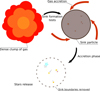 |
Fig. 1 Star formation process described by our new prescription, from the clump transformation into sink particles to stars release inside the simulation domain. This process is subdivided into three parts. First, a collapsing clump of gas passes tests to be transformed into a sink particle. The sink particle can accrete during tacc. After reaching this time, the sink is dissolved and its mass is shared to produce newborn stars at its last location. |
3.2 Stellar feedback: H II regions
Newborn stars inside active star-forming regions are connected with their natal environment. They inject both kinetic and thermal energy into their surroundings (referred to as stellar feedback; Krumholz et al. 2014), which can influence future star formation. Examples of momentum-driven feedback are jets or winds. Thermal feedback occurs from stellar irradiation.
Irradiation consists of two main components: ionising and non-ionising radiation. Non-ionising radiation from direct stars or dust-reprocessed light can heat the gas via absorption. It occurs mostly at infrared wavelengths around dense cores hosting protostars, where the gas starts to be optically thick (Bate 2009). Ionising radiation is produced by massive stars (>8 M⊙) inside molecular clouds. Photons with energy larger than ELy = 13.2 eV can directly ionise hydrogen atoms. Ionised gas around massive stars is heated to 10 000 K (the result of heating and cooling equilibrium). It creates a strong temperature gradient with cold neutral gas inside the region, which consequently produces a strong pressure gradient. Thus, ionising radiation from massive stars produces bubbles of hot gas around them that will expand inside the star-forming region, creating what is called an H II region (Osterbrock & Ferland 2006). This is thought to drive gas expulsion from star-forming regions, a key element of young stellar cluster evolution.
N-body simulations (Kroupa et al. 2001) tried to model gas expulsion with simple methods such as an exponential decay ofa gravitational potential inside the star cluster. Since we modelled the gas directly, it is possible to model this feedback process by heating the gas around massive stars inside the newborn cluster. Models trying to reproduce H II regions already exist and have been used in numerical simulations from the Galactic scale to the near-neighbourhood of massive stars. They can be modelled with more or less precision depending on trade-offs that authors made between accuracy and performance in agreement with their physical constraints. For example, Hopkins et al. (2012) used a coarse model to implement H II region feedback from entire star-forming regions to probe their effects on a global galaxy simulation without killing numerical performance. At the more sophisticated end, radiation transfer specialised codes are used in Dale et al. (2012) and Verliat et al. (2022) to precisely model ionising photon propagation inside a specific star-forming region to resolve the coupling between star formation and stellar feedback. However, such schemes come with a large numerical cost. Since we aimed to be computationally efficient while conserving individual star resolution, we wanted to model each H II region produced by massive stars inside one simulation.
To achieve this, we implemented a model similar to that of Fujii et al. (2021) and González-Samaniego & Vazquez-Semadeni (2020) to simulate individual massive star H II regions inside star-forming regions. This method is based on a distribution of the ionising photon rate produced by massive stars (>8 M⊙) at each SPH particle around them, assuming ionisation equilibrium inside the hot region and neglecting diffusion. If the ionising rate is sufficient to completely ionise a particle, the particle is tagged as ionised and its temperature and sound speed are changed accordingly. If not, it means that the ionisation front is nearby and all particles inside the H II region have been tagged as ionised.
Each massive star (>8 M⊙) ionising photon rate, ΔΝ, was computed using a fit function of the mass proposed in Fujii et al. (2021) and based on observational surveys. Then, at each simulation update, an iterative algorithm verified if the nearest SPH particles of a massive star were ionised or not. The algorithm computed the ionising photon rate to fully ionise the massive particle. Following Hopkins et al. (2012), it gives
 (34)
(34)
where mi is the particle mass, μ the mean molecular weight, mp, the proton mass, αβ ≈ 2.3 × 10⁻¹³cm3s−1 the recombination rate, and np the number density. If δΝp < ΔΝ, the particle was ionised and δΝp was subtracted from ΔΝ. Then the algorithm was repeated on the next nearest particle until δΝp > ΔΝ. Reaching this point, the H II region was sampled. The algorithm was applied to each massive star in the simulation. To help the algorithm, nearest-neighbour lists of massive stars were constructed using the tree-walking routine from Phantom.
In contrast to the method described by Bisbas et al. (2009) or Dale et al. (2012), we did not implement ray-tracing. Our method generates H II regions efficiently but also produces side effects when the mass resolution is not high enough to open H II regions in a very dense clump of gas or if a region starts to grow inside void (due to free boundaries in SPH). The first side effect can easily be avoided by increasing the resolution and/or attributing a fraction of the ionising temperature to the nearest particle to help the gas expand and consequently open the H II region. In the second side effect case, all ionising radiation will be focused where the gas is, as the iterative algorithm does not allow radiation escape. It could then potentially lead to an overestimate of the H II region. Our implementation follows what Fujii et al. (2021) proposed to minimise this effect by limiting H II regions to a size near the initial radius of the molecular cloud. Our tests to ensure convergence of the model following Bisbas et al. (2015) are presented in Appendix B.
3.3 Fiducial model
We studied one specific fudicial model of a giant massive molecular cloud collapse to characterise the new star formation prescription and the resulting star cluster. This model starts from an isolated isothermal massive turbulent molecular cloud. It is initially spherical, with a radius of Rc = 10 pc and a total mass of Mc = 104M⊙. A turbulent velocity field is initially injected into the cloud. We generated this using methods from Make-Cloud (Grudić 2021). It produces initial turbulence by applying a Gaussian random field filtered by a Larson-like power spectrum (Larson 1981) to the particle velocity. Compressive and solenoidal modes are introduced with proportions of 30% and 70%, respectively. This field is finally scaled to reach a turbulent virial ratio, αt = 2 (marginally stable condition). The cloud’s initial temperature is set to 10 K, and the mean molecular weight is set to μ = 2.35. This model ignored the magnetic field and external driving (pressure and turbulence). As the cloud is supposed to be isothermal, no cooling and heating processes are included, except photoionisation.
For the star formation prescription, the accretion radius, racc, and critical density, ρcrit, need to fulfil resolution criteria to ensure that gravitational collapse is resolved up to the sink scale. These two values then need to be chosen in agreement with the mass resolution of the simulation that gives the number of SPH particles. Our sink particle accretion radii should represent the characteristic size of a core in star-forming regions of a few thousand astronomical units (Sadavoy & Stahler 2017). Thus, we set the accretion radius to 4000 au. The critical density can then be computed using Eq. (33), which can then give a minimum mass resolution using Eq. (31) to resolve the collapse of clumps. The maximum critical density is equal to ρc = 1 × 10⁻¹⁸g cm−3 using an accretion radius of 4000 au. The coarsest mass resolution is around 0.009 M⊙, which gives a minimum SPH particle number of  million. Preliminary tests show that simulations close to this minimum number gave unusual accretion behaviours. A low number of particles cannot sufficiently retrieve small turbulence modes, causing faster artificial damping of turbulence, leading to early collapse. We therefore set the resolution to 3.5 million particles for this fiducial model. Finally, we set the sink accretion time to 0.5 Myr, and the star seeds formation time to 0.1 Myr, as is discussed in Sect. 3.1.
Sinks are created after the density exceeds the critical density and the tests to ensure that the clump collapses pass. This means that regions of cloud exceeding the critical density are not necessarily directly transformed into sinks. These tests avoid confusing isothermal compression that can increase the gas density without gravitational collapse. However, such isothermal compression can be expensive in numerical integrations. To accelerate the computation, one can force the sink creation after exceeding the critical density by a certain factor. In this model, the sink creation forcing is set to foverride = 100ρc. Table 1 summarises all parameters of this model.
Main parameters of the fiducial model.
4 Results
In this study, we evolved three simulations of this fiducial model with different initial turbulence states to 6.5–7 Myr. We denote the three simulations as embedded cluster formations 1, 2, and 3 (hereafter ECF1, ECF2, and ECF3) in the subsequent sections. Each simulation was computed in around 14 000 CPU hours, which corresponds to around 18 days of computation on one compute node (32 cores).
4.1 Qualitative description
Figure 2 shows all three simulations at different timestamps of their evolution, from the initial gas fall up to the star cluster emergence. Each row and column corresponds, respectively, to a specific simulation (top to bottom) and timestamp (left to right). Snapshots display the column density of the gas overlaid by sinks and star positions.
As was expected, the early evolution (t = 3 Myr) of each cloud is similar in each case. They start to diverge after the first star formation events. The first massive star formation presents a turning point in their evolution. These massive stars (>8 M⊙) open large H II regions around them. Their location and efficiency dramatically change the subsequent cloud collapse.
The first massive star is formed early in ECF1, around 1.5 Myr before reaching the initial freefall time. The resulting H II region pushes the gas outwards efficiently, inducing a significant compression in the cold molecular gas, causing it to collapse and trigger secondary star formation. In the meantime, other regions of the cloud continue their collapse and eventually produce other massive stars able to efficiently heat and ionise the cold gas with their strong radiation. Their accumulation accelerates the gas expulsion, leaving behind a new cluster of stars exposed from their parental cloud. Triggered formation following expanding bubbles is imprinted with their motion, resulting in a global expansion of the newly formed cluster.
ECF3 shows similar outcomes from ECF1, with a large expanding H II region hosting secondary formation at its outskirts. However, gas expulsion is more efficient. The final cluster appears correspondingly looser and more spatially extended. It did not produce massive stars early. Instead, the cloud collapse had more time to concentrate its mass in a central region. This stronger collapse produces multiple massive stars in a short time interval and in the same area. The coherent addition of H II regions leads to the most efficient gas expel and the highest cluster expansion rate seen in this work.
ECF2 produces a highly off-centre massive star early in the simulation in comparison to the other two. Its H II region expands slowly and pushes the gas gently, helping it to collapse naturally under its weight. Moreover, later-formed massive stars do not show coherent effects on their H II regions as in ECF3, even if these stars are the most massive ones in all simulations. Instead, shocks are produced between H II regions, thereby facilitating the condensation of cold gas to an even greater extent. With the help of gravitational collapse, this leads to the formation of a very compact cluster that is not yet fully revealed from its natal gas and where star formation is still ongoing at the end of the computation (~6.6 Myr).
The triggered formation has already been seen and studied in numerical simulations. Dale et al. (2012) performed molecular cloud collapse with H II feedback relatively similar to ours. They found in their simulation that ionising radiation from massive stars shapes the gas inside such molecular clouds by creating large bubbles and pillars, which are also observed here. They also concluded that this radiation feedback induced a significant rise in star formation, which also corroborates what is found in our simulations. However, their calculation stops rapidly (Model J) due to growing time step constraints on the stellar dynamics. Our new methods allow us to continue the calculation further. Thanks to this amelioration, we can now see that this triggered star formation can still happen far from the revealed cluster, creating an expanding distribution of low-mass stars around denser clusters.
The formation of massive stars, their spatial locations, and their coherent contributions are key elements in the future of a young stellar cluster that will be sculpted by H II region expansion. Their locations and masses are function of the initial turbulent velocity field and mass sharing inside sinks, which is random by definition. It means that the formation of such clusters is, similar to their evolution, highly stochastic. This confirms that a statistical study is necessary to identify the main evolutionary paths of embedded clusters.
4.2 Star formation efficiency
The gas mass conversion and its evolution in time can help characterise the star formation inside clouds. Dividing the converted mass by the initial gas mass gives an efficiency factor referred to as the star formation efficiency (SFE). This coefficient is an indicator of the evolutionary stage of a star-forming region and is computed at various scales in observational works, from 0.01 to 10 pc (Alves et al. 2007; Evans et al. 2014; Louvet et al. 2014; Könyves et al. 2015). From an entire giant molecular cloud to a smaller scale, such as in the neighbourhood of dense cores inside a larger complex, the definition of the SFE is the same and is given by
 (35)
(35)
where M* and Mcloud are the total mass of stars and the total mass of gas inside the considered region, respectively. In our study, SFE was computed at the cloud scale. Hence, no external mass was added to the calculation, which may not be the case in observations due to external gas inflows and protostellar outflows.
Figures 3, 4, and 5 show for each simulation the evolution over time of key parameters linked to the gas mass conversion into stars, namely the SFE (top panel), the median values of sinks mass and accretion rate (bottom left and centre), and the number of sinks and stars (bottom right). Each simulation reaches a SFE exceeding 10%, with values between 14% and 18%. These efficiencies are high compared to those observed in parsec-scale star-forming regions (see however Louvet et al. 2014). Such high efficiencies tend to be found at much smaller scales (e.g. Könyves et al. 2015, at 0.01 pc scales). This suggests that other feedback mechanisms, such as jets (Machida & Matsumoto 2012), or other physics such as non-ionising radiation and magnetic fields (Price & Bate 2009), may be needed to regulate the mass conversion. However, it is difficult to perform a direct comparison as real molecular clouds are certainly not in complete isolation and can gather gas inflow, which will reduce the SFE.
Most of the gas conversion occurs in ~2 Myr, between 4 and 6 Myr (0.75 to 1.13 τff). The first sinks appear around 3 Myr (0.56 τff) and are limited to a small number during one million years. The mean star formation rate (SFR), given by the mean slope of the mass conversion evolution in time, is equal to 6.8 × 10⁻⁴ Μ⊙ yr−1 for the first two runs. ECF3 shows a slightly lower value with 4.5 × 10⁻⁴ Μ⊙ yr−1. All three mass conversion slopes increase monotonously during the whole computation.
It is difficult to see where star formation halts from the number of sinks over time. In ECF2 and ECF3, the number of sinks starts to decrease at the last few points. This, in addition to the SFE slow down in both simulations, suggests that star formation is about to stop. By contrast, the number of sinks is still increasing in ECF1 and the SFE does not show any slow-down. This late increase is only due to secondary star formation in Η II regions outskirts. It could also be induced by numerical effects. It seems clear that simulations should be evolved further in time to determine when star formation stops (discussed in Section 5).
A key event occurs between 4 and 4.5 Myr (0.75 to 0.84 τff) for all calculations, when the star formation process produces a sharp rise in the number of sinks produced in the cloud. Except for ECF3, this moment coincides with the first formation of massive stars.
The median values of sink mass and accretion rate show two different regimes at the same turning point of 4Myr for ECF1 and ECF2. In ECF1, before this time, the mean value of the median for both plots is equal to 10 Μ⊙ yr−1 and 3 Μ⊙. These values drop to 2 Μ⊙ yr−1 and 0.8 Μ⊙ just after the turning point. The number of sinks also drastically increases from less than ten to more than a hundred in less than a million years after this timestamp. This sudden jump occurs due to the opening of an Η II region.
Expanding bubbles in these simulations greatly modify the star formation regime making a sharp transition from a dominant massive formation channel to a low-mass one, as observed in some evolved massive protoclusters (e.g. Armante et al. 2024). This new channel produced stars in the outskirts of H II bubbles where sinks and gas rapidly decouple after their formation. As sinks form, these only evolve through gravitational interaction and lose pressure support that drives H II bubble expansion. Thus, if this expansion accelerates, sinks do not have the time to accrete material before entering an ionised region where accretion is no longer possible. Most of the converted mass after the turning point then goes mostly into low-mass sinks, explaining the sharp transition.
In unperturbed locations of the cloud, massive stars still form following the natural cloud gravitational collapse. A revival of both the accretion rate and the mass can be seen to start at ~0.95 τff in ECF1 and ECF2. It reaches a maximum at ~ 1.05 τff that coincides with the most massive sink formation in both simulations. Higher revival in ECF2 also agrees with previous observations (see Section 4.1) that showed that Η II bubble expansion was gentler, leading to a forced collapse instead of a dismantling. ECF2 produces the most massive sink and then the most massive star with a mass of 180 Μ⊙ and 45 Μ⊙, respectively. It seems logical that regions unaffected by Η II bubbles will collapse very rapidly and efficiently near the initial free-fall time. The behaviour of the ECF1 and ECF2 runs reminds the Aquila and W43 protoclusters (Könyves et al. 2015; Motte et al. 2003).
In comparison, ECF3 do not produce early massive stars like the other two. This particular simulation shows a smoother formation process up to τff, perhaps resembling the star formation activity in nearby, low-mass star-forming regions. It follows the gravitational collapse of the cloud that naturally accelerates. Thus, the number of formed sinks increases smoothly. The lack of forcing by the H II region prevents the sharp transition at 0.75 τff as in the other runs. The acceleration of the collapse stops sharply at ~1.05 τff. As many massive sinks were able to cluster in dense regions without any feedback, this led to the simultaneous formation of massive stars in the same region. This burst of massive star formation produces the sharpest regime transition observed in the simulations, permitting solely low-mass star formation until the end of the computation. However, this scenario is probably not the sole possibility if early massive star formation does not occur. Finally, the SFE of this simulation is the lowest, which may be due to rapid gas removal. This may correlate with a conclusion made by Dale et al. (2012), who link a lower SFE to efficient photoionisation feedback.
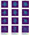 |
Fig. 2 Snapshots showing the evolution of three fiducial clouds computed at multiple time steps. Each column corresponds to a specific run (top: ECF1, middle: ECF2, bottom: ECF3) and rows give different epochs in each of them. The colour map gives the z integrated column density of the gas in M⊙ pc−2, while red circles correspond to sink positions and stars are coloured using realistic black body temperature extrapolated from a luminosity-mass relation. ECF1 presents a protostellar cluster under the influence of Η II regions distributed in various parts of the molecular cloud; for instance, Aquila. ECF2 presents a more centrally concentrated protostellar cluster, which develops a cluster of Η II regions, such as the region W43. ECF3 is more difficult to link with an existing star-forming region. As all the gas has been removed very rapidly, the resulting group of stars looks like a more evolved association or cluster such as NGC 6611. |
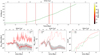 |
Fig. 3 Evolution over time of multiple key parameters linked to the gas-to-star mass conversion. The top panel shows the time evolution of the mass of gas converted in sinks and stars in ECF1. The formation of massive stars is represented by vertical lines, with their colour indicating the mass of the massive object. The bottom panels show the temporal evolution of the accretion rate (left), mass median (centre), and the number of stars and sinks formed in the simulation (right). For the first two panels, the quartile range (grey zone) and the maximum value (dashed line) are also shown. It allows us to see that the sharp transition at 4Myr occurs on the majority of sinks. However, even after the change of regime, the cloud is still capable of producing some massive sinks with a high accretion rate. |
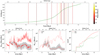 |
Fig. 4 Same as previous figure, but applied to the ECF2 simulation. |
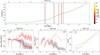 |
Fig. 5 Same as previous figure, but applied to the ECF3 simulation. |
5 Discussion
5.1 Numerical performance
In terms of computational efficiency, we find our new N-body and H II region implementations to be effective at speeding up the calculation when the stellar environment densities. Our new subgroup methods correctly handle every close encounter or binary. ECF2, which shows the densest cluster formed in this study, produces a maximum of 17 subgroups involving 38 stars at the same snapshot. Even if this number is small compared to the total number of stars at the end of the simulation (Nfinal = 1225), the performance boost is significant, as only one of these subgroups can impose a time step that is orders of magnitude lower in the substep loop. We indeed observe one bound group that has a time step a hundred times smaller than the minimal time step with no subgroup integration with a minimum separation of 4 au.
To properly demonstrate this performance boost, we relaunched the simulation near the time of creation of this hard binary. This new calculation took 48 hours (walltime) to complete only one fifth of the time integration until the next dump. In comparison, the whole time integration took 3.1 hours with our new implementation, which gives a gain of approximately 80. The gain depends on the hardest binary in the system.
With our methods, time step constraints set by individual stars (not in subgroups) are always close to the CFL (Courant-Friedrich-Lewy) constraint (Courant et al. 1928) of the densest SPH particles in the cloud during the simulation, which sets the slow force minimum time step, i.e. the number of substeps is always contained to a reasonable number (a few tens at maximum). Hence, none of these parts of the calculation is a major bottleneck.
The main performance hit is due to the interactions between point masses (sink and star) and the gas. These are calculated with a direct method in Phantom and always at the lowest time step of the scheme. In most applications of Phantom to date, this part of the algorithm was not the main bottleneck, as the sink number was not large enough for the 𝓞(NsinkNgas) interaction to dominate the complexity. Such interactions essentially scale linearly with particle numbers in our simulations, as in previous studies. As a result, this bottleneck makes the computation too expensive to go further in time than 6 to 7 Myr for our application.
Since the number of point masses is close to three thousand in our simulations, these interactions start to dominate the computational expense. As said above, they are also computed for every point mass at every time step, even when only a few gas particles are active in the individual time stepping scheme. It is a waste of computation time, as the time step constraints of sink or star and the gas interactions are often two or three orders of magnitude higher than the smallest one. On average, this part of the calculation represented more than 80% of the computation time of one global step when the number of sinks is higher than ~ 1000. This bottleneck is the main remaining limitation that makes it difficult to carry out this type of simulation on a statistical scale, which is the ultimate goal of the project. Future work will focus on optimising this part of the calculations. For example, following what has already been done in collisional N-body codes (Mukherjee et al. 2021; Wang et al. 2020a), these forces – as they do not strongly perturb the evolution of hard groups or close encounters – can be computed with the help of the Phantom kd-tree reducing the complexity to 𝓞(Nsinklog(Ngas) + Ngaslog(Nsink)) and/or by only computing these forces at the first integration level. The latter solution would make it possible to avoid computing these interactions multiple times during the substep scheme, and computing them only once per step should save most of the unnecessary calculations.
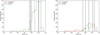 |
Fig. 6 Histograms of the number of sinks over time. The red histogram gives the formation of sinks passing every test. The green histogram gives the forced sinks. Vertical dashed lines represent massive star formation. ECF1 is on the left panel and the right panel is the same initial conditions with foverride set to 1000 referred to as ECF1B. |
5.2 Effect of foverride on sink formation output
We investigated the effect of the foverride parameter used to force the creation of a sink if an SPH particle reaches the critical density without passing other physical tests detailed in Price et al. (2018) or Bate et al. (1995). These tests check whether the gas clump is indeed starting to collapse gravitationally, or whether it is just experiencing hydrodynamical compression. If the gas is isothermal, such compression can rise several orders of magnitude higher than the critical density. In our simulations, high density implies high time constraints that will drastically slow down the computation. Moreover, all this extra cost is unnecessary, as the critical density is supposed to be close to the maximum resolution of the simulation. The extra computation above the critical density is not guaranteed to be physically accurate, foverride is therefore here to force the creation of a sink after reaching
 (36)
(36)
with foverride equal to several orders of magnitude to find a good compromise between efficiency and accuracy.
For the sake of efficiency, this parameter was set to 100 in the simulations of this paper, but this is a relatively low value. With this value, HII region expansions produced in the simulations show efficient sink formation at the outskirts of these regions. The compression induced by hot bubbles in the cold collapsing gas can force this collapse and lead to a burst of sink production. However, it can also produce compression in non-collapsing regions that can exceed the critical density. Therefore, we find that a too low foverride parameter could overestimate this burst of sink production, leading to an overestimated number of low-mass stars at the end.
Figure 6 shows histograms of the formation of sinks over time, and up to one freefall time, of two simulations with different foverride Values (ECF1 With foverride = 100 and ECF1 With foverride = 1000). ECF1 produces all its sinks, except one, via forced creation. Looking at ECF1B, we see that the first sink creations are similar. Thus, the forced creation does not overestimate the production of sinks during the initial collapse. The sink productions of ECF1 and ECF1B start to diverge after the first massive star formation. The total number of sinks produced after this timestamp is 263 (only forced) and 141 (79 standard and 62 forced) for ECF1 and ECF1B, respectively. Compared to ECF1B, ECF1 overestimates by at least 1.9 times its sink production at the outskirts of H II regions with foverride set to 100. While some of the forced sink creations are physical, and not numerical artefacts, a higher value of foverride helps to minimise this numerical side-effect. Therefore, foverride should be set higher than 100 in future simulations while keeping numerical efficiency in mind.
5.3 Sink merging
As was mentioned in Sect. 3.1, sinks can collide with others during their accretion phase. If two sinks collide and both encompass their centre of mass, they fulfil the conditions for a sink merger. In such a case, the two sinks are merged to form a new sink that inherits the physical properties of its parents. The new position and velocity are the barycentres between the two parents. This ensures the conservation of linear momentum during the simulation. The angular momentum is also conserved as Phantom tracks the spin of all sinks in the simulation. The sink properties provided by our new star formation prescription are also updated during a merger (see Section 3.1). In particular, the number of seeds in the initial sinks is summed into the merged sink.
Mergers are quite common in these simulations. The gravitational pull of the cloud tends to bring sinks closer over time, which inevitably creates collision trajectories between them. Mergers are key to forming very massive sinks that can then create massive stars. This merging process can take place consecutively on the same sink, leading to very massive sinks (the most massive one reaches 180 M⊙ in ECF2). Accretion rates measured in these simulations are too low without merger events to explain the formation of stars of 20–40 M⊙, which are essential to rapidly remove the gas from the star-forming region with their H II feedback.
In these cases, summing the parents’ star seeds can bring their number to a few dozen in a single sink (50 at maximum in ECF2). This can be seen as a contradiction with our main prescription hypothesis that permits only a few star seeds (fewer than five in these simulations) in a sink. This means that the most massive sinks need to share their mass with a large number of stars during the release phase. Randomness during sharing is smoothed in such cases, as it needs to cut the parent mass into more parts. As a result, most massive sinks create a large number of intermediate-mass stars. This is at odds with our model, which predicts that the most massive stars are produced inside very massive sinks. Therefore, our random sharing of mass between star seeds can bias the final star mass spectrum by undersampling high-mass stars and oversampling intermediate-mass stars. Since less massive stars also imply less feedback, it can also have an impact on the SFE and dynamics inside the star-forming region. Ultimately, we need to improve the merging process in relation to our new star formation scheme to make sure that the number of seeds inside a sink is always in agreement with the maximum value allowed; for example, by adding star escapers after a merging and/or modelling seeds merging inside our subgrid model.
6 Conclusions
This paper presents a new implementation of direct N-body algorithms as well as prescriptions for star formation and stellar feedback in the SPH code Phantom. Together, they unlock the possibility of studying embedded star cluster evolution from their birth inside a molecular cloud to their unveiling from their natal gaseous environment. The new algorithms come in two parts:
First, our new star formation prescription was implemented, which provides distributions of stars self-consistently formed from molecular cloud collapse at a low computational cost. It uses sink particles a thousand astronomical units in diameter that host star seeds within them and are transformed into stars after passing some criteria.
Second, we completely refactored the point mass time integration methods in Phantom. We replaced the existing second-order Leapfrog integrator with an accurate fourth-order FSI, which is now the default in the public code. Its symplectic properties guarantee conservation of angular momentum up to machine precision and good conservation of energy. Its forward properties also guarantee that there is no issue with dissipative forces in the code. In addition to this new integrator, we implemented specific methods (regularisation integration and slow-down method) to follow the true dynamics of binaries and multiples, which is an essential element of cluster dynamics.
In this paper, we performed a first study of massive star cluster formation to benchmark the method. We focused on a single fiducial model starting from a massive turbulent molecular cloud of 104 M⊙ mass and 10 pc radius. Three simulations with different random initial turbulent conditions were computed with the following results:
We find H II regions – more precisely those formed first in the simulation – to be the main game changers for the time evolution and spatial distribution of star formation inside these clouds. Their strength and location can completely change the future of a star-forming region. We find that the formation of an H II region can lead either to a very loose, globally expanding cluster in the case of efficient ionisation, or a very compact cluster when H II regions are off-centre and help the gravitational focusing of the cloud;
As a corollary to our first conclusion, since the early formation of H II regions is a stochastic process, we find the global evolution of such a cluster to be more stochastic than when just accounting for stellar dynamics. A suite of simulations is thus needed to obtain statistically robust outcomes;
We find the SFE in our simulations to be slightly high compared to observations, with the mass conversion of gas into stars also not finished at the end of our calculations. However, the effect of our H II feedback on the SFE corroborates previous studies. Adding new physical processes, such as magnetic fields, and feedback processes including non-ionising radiation, jets, and cloud motions associated with Galactic shear, should help to reduce the SFE.
These self-consistent simulations of the formation and early evolution of embedded clusters improve previous pure N-body simulations. The aim of these is to scale up the number of simulations performed to produce statistically significant results on the dynamical evolution of clusters under the direct influence of their natal environment. Paper II will aim to characterise the star formation prescription outcomes, especially stellar mass distributions and multiplicity properties, by exploring its parameter space with a larger set of simulations. This will potentially require refinements to generate a distribution of primordial binaries in the actual prescription. On the other hand, another study will be performed on high-resolution star formation simulations to connect dynamical properties seen below our sink scale to our prescription parameters. The new methods presented here solve performance bottlenecks that have previously limited such studies. New optimisations on gas-sink interactions may further accelerate the computation. The aim is to carry out around a hundred simulations over an integration period of between 10 Myr and 20 Myr to have clusters with fully dispersed gas at final outputs. Ultimately, we plan to study the dynamical evolution of young clusters through statistical analysis by producing a large grid of simulations to explore a vast initial parameter space. These simulations could then be compared with observations of young clusters, including the latest data available from Gaia.
Acknowledgements
We acknowledge M. Vaileille-Manet for his participation during the redaction of this paper. We thank the Australian-French Association for Research and Innovation (AFRAN) for financial support towards the 5th Franco-Australian Phantom users workshop held in Melbourne. DJP acknowledges Australian Research Council funding via DP220103767 and DP240103290 and thanks IPAG for hosting and financial support from both Monash and IPAG during his 2025 sabbatical in Grenoble where this paper was completed. YB thanks LabEx OSUG@2020 (Investissements d’Avenir – ANR10 LABX56) and IDEX for funding a 2-month mobility grant at Monash University. All the computations presented in this paper were performed using the GRICAD infrastructure (https://gricad.univ-grenoble-alpes.fr), which is supported by Grenoble research communities. F.M., F.L. and I.J. acknowledge funding from the European Research Council (ERC) via the ERC Synergy Grant ECOGAL (grant 855130) and from the French Agence Nationale de la Recherche (ANR) through the project COSMHIC (ANR-20-CE31-0009). We used SPLASH and Sarracen for many of the figures presented above.(Price 2007; Harris & Tricco 2023).
Appendix A Details of N-body methods
A.1 FSI derivation and accuracy
The original Leapfrog algorithm used in Phantom can be easily derived using the Hamiltonian formalism to write the equation of motion of the studied system. This equation can be written as
 (A.1)
(A.1)
where w is the phase space vector of the system, H is the system Hamiltonian and {,} is the Poisson brackets operator. The formal solution of this equation over a certain time interval δt is then straightforwardly given by
 (A.2)
(A.2)
where eδtH is an operator that evolves the system in time. All symplectic integrators come from a particular way to approximate this time evolution operator. Indeed, it can be reformulated into a product decomposition with a specific Hamiltonian that can be split into two parts, for example, a kinetic part Τ and a potential part U. It gives
 (A.3)
(A.3)
where Nsub corresponds to the number of subdivisions of the time evolution operator. cki and dki are coefficients (also called symplectic coefficients) that weigh the decomposition into multiple parts. The sums of these two series of coefficients need to be equal to 1 to respect the decomposition. The resulting two operator types can be associated with different steps in the time evolution. U potential is always associated with a force applied to the system using eδtU. eδtU is only applied to momentum co-ordinates,
 (A.4)
(A.4)
This operation is called a kick. eδtT represent the inertial part of the evolution. It will then only modify positions depending on velocities
 (A.5)
(A.5)
This operation is called a drift. A system can be integrated into a given time following a succession of alternating kick and drift operations using this decomposition method. The number of kick and drift operations Nsub and a couple of coefficients (cki, dki) give the integrator order of truncation. for the Leapfrog, Nsub = 2 and (ck1, dk1 = (1, 1/2) or (1/2, 1) and (ck2, dk2) = (0, 1/2) or (1/2, 0) depending on the order of the kick and drift operations. The number of operations and the symplectic coefficients can be efficiently found (Yoshida 1990) with the Campbell-Baker-Hausdorff (CBH) formula (Campbell 1896; Baker 1905), namely
![Mathematical equation: $\matrix{ {\log \left( {{e^X}{e^Y}} \right) = X + Y + {1 \over 2}\left[ {X,Y} \right]} \hfill \cr {\,\,\,\,\,\,\,\, + {1 \over {12}}\left( {\left[ {X,\left[ {X,Y} \right]} \right] + \left[ {Y,\left[ {Y,X} \right]} \right]} \right) + O\left( {X,Y,\left[ {X,Y} \right]} \right).} \hfill \cr } $](/articles/aa/full_html/2025/10/aa54938-25/aa54938-25-eq46.png) (A.6)
(A.6)
Substituting the left hand of Equation (A.3) into Equation (A.6), one finds
![Mathematical equation: $\eqalign{ & \log (\prod\limits_{i = 1}^{{N_{{\rm{sub}}}}} {{e^{\delta t\;{c_{{\rm{ki}}}}\;T}}{e^{\delta t\;{d_{{\rm{ki}}}}\;U}}} ) = \delta t({e_c}T + {e_d}U + {{\delta t} \over 2}{e_{cd}}\left[ {T,U} \right] \cr & \;\;\;\;\;\;\;\;\;\;\;\;\;\;\;\;\;\;\;\;\;\;\;\;\;\;\;\;\; + \;{{\delta t} \over {12}}({e_{ccd}}\left[ {T,\left[ {T,U} \right]} \right] + {e_{dcd}}\left[ {U,\left[ {T,U} \right]} \right]) \cr & \;\;\;\;\;\;\;\;\;\;\;\;\;\;\;\;\;\;\;\;\;\;\;\;\;\;\;\;\; + \;O(T,U\left[ {T,U} \right]), \cr} $](/articles/aa/full_html/2025/10/aa54938-25/aa54938-25-eq47.png) (A.7)
(A.7)
where all e prefactors are called error coefficients and are functions of (cki, dki). The first two coefficients correspond to the sum of cki and dki, which by definition needs to equal unity. Thus, ec and ed are equal to unity. One can refactor Equation (A.7) using these equalities according to
![Mathematical equation: $\log \left( {\mathop \prod \limits_{i = 1}^{{N_{{\rm{sub}}}}} {e^{\delta t\,{c_{{\rm{ki}}}}\,T}}{e^{\delta t\,{d_{{\rm{ki}}}}\,U}}} \right) = \delta t\left[ {H + {H_{{\rm{err}}}}\left( {\delta t} \right)} \right] = \delta t{H_{{\rm{neigh}}}}.$](/articles/aa/full_html/2025/10/aa54938-25/aa54938-25-eq48.png) (A.8)
(A.8)
This new form hints at what is needed for a symplectic integration. What is evolved in such a scheme is not the true Hamiltonian, H, but a neighbour of this one, Hneigh, which differs from an error called Herr. The goal of constructing high-order symplectic integrators is then to minimise this error quantity by setting the next error coefficients to zero. However, it has been proven (Sheng 1989; Suzuki 1991) that after second order (cki, dki) coefficients must contain some negative values to set the next order coefficient to zero. However, negative time steps are problematic when integrating dissipative systems that are common in astrophysics. The solution proposed by Suzuki (1991) was to add one of the first terms of the error Hamiltonian produced by a Leapfrog scheme into the true one. One can then erase all error terms of the fourth order. Nonetheless, the part added to the classical Hamiltonian still needs to be computed. It is possible to write the new Hamiltonian as
![Mathematical equation: $H = T + U + {1 \over {48}}\delta {t^2}\left[ {U,\left[ {T,U} \right]} \right].$](/articles/aa/full_html/2025/10/aa54938-25/aa54938-25-eq49.png) (A.9)
(A.9)
In this equation, [U, [T, U]] is a composition of two commutators between U and Τ. Dehnen & Hernandez (2017) showed that this commutator corresponds to an extra potential quantity in the Hamiltonian defined as
![Mathematical equation: $\left[ {U,\left[ {T,U} \right]} \right] = - \mathop \sum \limits_i^N {1 \over {{m_i}}}{\left( {{{\partial U} \over {\partial {r_i}}}} \right)^2} = - \mathop \sum \limits_i^N {m_i}{a_i}.$](/articles/aa/full_html/2025/10/aa54938-25/aa54938-25-eq50.png) (A.10)
(A.10)
Figures A.1a and A.1b illustrate the superior accuracy of the FSI method by showing the trajectory of one point mass around a fixed gravitational potential during 10 orbits and its energy conservation (logarithm of the relative energy) for one orbit, respectively. FSI1 and FSI2 correspond, respectively, to the original gradient force calculation and the extrapolation method. The initial eccentricity of the body is large (e = 0.7) to show the orbital precession that can be introduced by numerical error. A large time step is also deliberately chosen (around 60 steps per orbit) to amplify numerical imprecision. As expected, energy conservation and orbit precession are much improved with a fourth-order scheme than with a simple leapfrog scheme. It also confirms the Chin & Chen (2005) result that forward schemes have better conservation properties.
 |
Fig. A.1 Evolution of a point mass around a fixed potential |
A.2 Few-body problem regularised by TTL
Let’s introduce a general N-body (only Newtonian) system hereafter regularised with the Time Transformed Leapfrog (TTL) scheme. The equations of motion are given by
 (A.11)
where N is the number of bodies and G the gravitational constant and rij is the distance between body i and j. For convenience G = 1. Now, let’s introduce the time transformation
 (A.12)
where Ω(r) is an arbitrary time transformation function. To follow what is done in Mikkola & Aarseth (2002) and Wang et al. (2020b), this function can be defined as
 (A.13)
One can now set a new auxiliary variable, often called W = Ω, to rewrite the system according to
 (A.14)
 (A.15)
 (A.16)
where index i indicates one body of the system. The addition of a new variable gives a supplementary variable in the system that can be extracted from the differential equations.
 (A.17)
which can be expressed using our new ‘time’ co-ordinate,
 (A.18)
This new variable W acts like an associated momentum for the time, which means that it will have the same behaviour as a velocity in a symplectic scheme. With that in mind, it is then possible to form one drift and one kick operation from this system, given, respectively, by
 (A.19)
 (A.20)
where ck is the drift coefficient and δt is the time step. Then
 (A.21)
 (A.22)
 (A.23)
where dk is the kick coefficient and * represents updated variables. As W depends on the velocities of each body, it is needed to update both variables simultaneously. To achieve that, the velocity kick is split in half with a W kick between the two parts. These two operations can be successively applied to the system to integrate its motion using any kind of symplectic integrator.
A.3 Discussion on slow-down factor
As has been shown above, κ quantifies the number of original periods where the perturbation applied to the binary can be averaged. On a highly perturbed binary, it is impossible to average the perturbation on multiple periods, which means κ = 1. On the other side, a hard binary can stay unperturbed during a whole simulation. The averaging is not risky at all, and then κ can stay at a high value. That being said, one can see that this factor needs to scale with the strength of the perturbation. The solution proposed originally by Mikkola & Aarseth (1996) is to compute the relative tidal perturbation at the maximum apocenter (2a with e = 1), giving
 (A.24)
where a is the semi major axis of the binary, p and s point on the binary components. rbj is the distance between any perturbers and the binary centre of mass. κ value is then equal to
 (A.25)
where γ0 is a safety factor to adjust the precision wanted by the user, often chosen between 105 and 106. Wang et al. (2020b) chose something slightly different for this quantity. In their work, they proposed
 (A.26)
Instead of using the maximum possible apocenter of the binary, they chose the actual apocenter. The most different part of their proposition is the summation. They directly sum the cubed distances scaled by the mass of each perturber. Even if these two expressions look similar, they have totally different behaviour. For example, let’s consider a system composed of one hard binary that can be slowed down and two single perturbers. To simplify the system, each bodies have the same mass. One perturber is far from the binary, producing weak perturbations. The other one is on a hyperbolic trajectory with the binary close to its periapsis. It then produces a strong perturbation. In theory, this scenario should produce a slow-down factor near unity due to the close encounter with perturber two. The first expression will first sum the inverse cube distance, which will give a large number (since the strong perturber dominates the summation). Taking the inverse of this summation gives a number less than unity (which means no slow-down in this framework). The first expression has good behaviour, but with the second expression, the dominant perturber is the weaker one, which will give a high κ value. This expression is then potentially wrong. Therefore, in this work, we stuck with the original expression, which leads to more robust behaviour by changing only the apocenter expression.
Finally, the κ value of each binary in the system needs to be updated regarding the perturbation modification in the system. However, this evolution needs to be slow to conserve the secular evolution properties. Wang et al. (2020b) proposed a limit value for κ that is controlled by the changing rate of the perturbation. Formally, it is written as
 (A.27)
where c = 0.1 is a safety factor, P is the period of the binary, vbj is the relative velocity vector between perturbers and the binary CoM. 〈〉m refers to a mass-weighted average.
Appendix B HII region unit test
We performed a simple test in order to validate the HII feedback implemented into this work, following what was proposed in Bisbas et al. (2015). They described two main set-ups to check the validity of HII region expansion on two different timescales (early and late) compared to analytical solutions. Such solutions exist only in very specific and simple systems. The selected test (late) tries to expand an HII region produced by a 40M⊙ star in the centre of a homogeneous sphere of hydrogen atomic gas of 2.9pc in radius. Here, we set the cloud mass to 8 × 10M⊙, which was divided into 8 million SPH particles. The neutral temperature was set to 1000 K. Boundary particles are also mandatory at the edge of the cloud to avoid relaxing into empty space, which could lead to an artificial acceleration of the HII bubble. Figure B.1 plots the HII region radius derived by Phantom, while Figure B.2 shows a density slice of the cloud. Our implementation agrees with the Bisbas et al. (2015) analytical solution during 0.6Myr and comes close to the stagnation radius equal to 2.31 pc. The sudden drop after 0.6Myr is due to the shock front reflecting from boundary particles, which compresses the HII bubble, forcing it to shrink suddenly. This phenomenon is not present in Bisbas et al. (2015) work. Nothing is detailed on boundary conditions for SPH runs. Nonetheless, the satisfactory agreement on the first part is sufficient to validate the implementation, as boundary conditions in large clouds have already been tackled in 3.2.
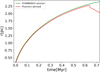 |
Fig. B.1 Time evolution of the HII region front radius. The green line is the analytical solution found in Bisbas et al. (2015). The red line is the Phantom-derived solution. The sudden drop after 0.6 Myr is due to the front shock reflection onto the boundary particles. |
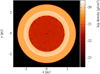 |
Fig. B.2 Density slice of a uniform density sphere where a HII region expands from its centre. A central stellar object produces many ionising photons that heat the gas around it. Two media (hot and cold) are separated by a front shock that propagates inside the cold sphere, sweeping up the gas. A denser shell of material forms just next to the ionisation front. |
Appendix C SDAR unit test
We performed a unit test taken from Wang et al. (2020b) to validate our SDAR implementation. This test consists of a hierarchical triple system (binary-single) with a hard eccentric inner binary orbiting another single star. The outer orbit is eccentric as well, with a semi-major axis ratio of 1000 between the inner and outer binary. All orbital parameters are summarised in Table 1 of Wang et al. (2020b).
Kozai-Lidov oscillations (Kozai 1962; Lidov 1962)) are expected on the inner eccentricity and inclination in such systems as the outer star will perturb the inner binary at each periapsis. Such a system is a good test to verify if our SDAR module can correctly model this oscillation with and without the slow-down method. Figure C.1 shows the eccentricity of the inner binary over time. As expected, A clear oscillation between 0.9 and 1. is visible, and both methods converge on the same solution. Figure C.2 shows the evolution of κ slow-down factor over time. This one oscillates between around 50 and 1 depending on the outer binary orbital phase. If the single outer star is at apoapsis, its perturbation on the inner binary is minimal; therefore, κ is high. Its value decreases accordingly down to 1 as the star reaches the periapsis of the outer orbit. In this configuration, the perturbation is maximal. Hence, slowing down the inner binary is not possible. These results also converge with what was found in Wang et al. (2020b).
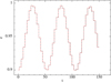 |
Fig. C.1 Time evolution of the inner binary eccentricity. This eccentricity oscillates under the perturbation of the single star orbiting the binary in a very eccentric orbit. |
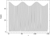 |
Fig. C.2 Time evolution of the slow-down factor κ. This one oscillates on a shorter timescale that corresponds to the outer binary period. When the single star reaches the apoapsis of its orbit. κ reaches its maximum at this moment. Oppositely and as expected, κ decreases during its descent to the periapsis. At this moment, slowing the inner binary motion is not possible; therefore, κ = 1. |
References
- Aarseth, S. J. 1999, PASP, 111, 1333 [NASA ADS] [CrossRef] [Google Scholar]
- Aarseth, S. J. 2003, in IAU Symposium, 208, Astrophysical Supercomputing using Particle Simulations, eds. J. Makino & P. Hut, 295 [Google Scholar]
- Aarseth, S. J., & Hills, J. G. 1972, A&A, 21, 255 [NASA ADS] [Google Scholar]
- Aarseth, S. J., Henon, M., & Wielen, R. 1974, A&A, 37, 183 [NASA ADS] [Google Scholar]
- Ahmad, A., González, M., Hennebelle, P., & Commerçon, B. 2024, A&A, 687, A90 [NASA ADS] [CrossRef] [EDP Sciences] [Google Scholar]
- Alves, J., Lombardi, M., & Lada, C. J. 2007, A&A, 462, L17 [NASA ADS] [CrossRef] [EDP Sciences] [Google Scholar]
- André, P., Di Francesco, J., Ward-Thompson, D., et al. 2014, in Protostars and Planets VI, eds. H. Beuther, R. S. Klessen, C. P. Dullemond, & T. Henning, 27 [Google Scholar]
- Armante, M., Gusdorf, A., Louvet, F., et al. 2024, A&A, 686, A122 [NASA ADS] [CrossRef] [EDP Sciences] [Google Scholar]
- Baker, H. F. 1905, Proc. Lond. Math. Soc., s2-3, 24 [Google Scholar]
- Bastian, N., & Goodwin, S. P. 2006, MNRAS, 369, L9 [NASA ADS] [CrossRef] [Google Scholar]
- Bate, M. R. 1998, ApJ, 508, L95 [NASA ADS] [CrossRef] [Google Scholar]
- Bate, M. R. 2009, MNRAS, 392, 1363 [CrossRef] [Google Scholar]
- Bate, M. R., & Burkert, A. 1997, MNRAS, 288, 1060 [NASA ADS] [CrossRef] [Google Scholar]
- Bate, M. R., & Bonnell, I. A. 2005, MNRAS, 356, 1201 [Google Scholar]
- Bate, M. R., Bonnell, I. A., & Price, N. M. 1995, MNRAS, 277, 362 [Google Scholar]
- Bate, M. R., Bonnell, I. A., & Bromm, V. 2002, MNRAS, 336, 705 [Google Scholar]
- Bate, M. R., Tricco, T. S., & Price, D. J. 2014, MNRAS, 437, 77 [NASA ADS] [CrossRef] [Google Scholar]
- Bisbas, T. G., Wünsch, R., Whitworth, A. P., & Hubber, D. A. 2009, A&A, 497, 649 [NASA ADS] [CrossRef] [EDP Sciences] [Google Scholar]
- Bisbas, T. G., Haworth, T. J., Williams, R. J. R., et al. 2015, MNRAS, 453, 1324 [NASA ADS] [CrossRef] [Google Scholar]
- Bleuler, A., & Teyssier, R. 2014, MNRAS, 445, 4015 [Google Scholar]
- Boss, A. P., & Bodenheimer, P. 1979, ApJ, 234, 289 [NASA ADS] [CrossRef] [Google Scholar]
- Bulirsch, R., & Stoer, J. 1966, Numer. Math., 8, 1 [CrossRef] [Google Scholar]
- Campbell, J. E. 1896, Proc. Lond. Math. Soc., s1–28, 381 [Google Scholar]
- Cartwright, A., & Whitworth, A. P. 2004, MNRAS, 348, 589 [Google Scholar]
- Chin, S. A., & Chen, C. R. 2005, Celest. Mech. Dyn. Astron., 91, 301 [Google Scholar]
- Courant, R., Friedrichs, K., & Lewy, H. 1928, Math. Ann., 100, 32 [Google Scholar]
- Cuello, N., Ménard, F., & Price, D. J. 2023, Eur. Phys. J. Plus, 138, 11 [NASA ADS] [CrossRef] [Google Scholar]
- Dale, J. E., Ercolano, B., & Bonnell, I. A. 2012, MNRAS, 427, 2852 [NASA ADS] [CrossRef] [Google Scholar]
- Dehnen, W., & Read, J. I. 2011, Eur. Phys. J. Plus, 126, 55 [Google Scholar]
- Dehnen, W., & Hernandez, D. M. 2017, MNRAS, 465, 1201 [NASA ADS] [CrossRef] [Google Scholar]
- Dunham, M. M., Allen, L. E., Evans, Neal J., I., et al. 2015, ApJS, 220, 11 [Google Scholar]
- Evans, Neal J., I., Dunham, M. M., Jørgensen, J. K., et al. 2009, ApJS, 181, 321 [NASA ADS] [CrossRef] [Google Scholar]
- Evans, II, N. J., Heiderman, A., & Vutisalchavakul, N. 2014, ApJ, 782, 114 [CrossRef] [Google Scholar]
- Forest, E., & Ruth, R. D. 1990, Physica D Nonlinear Phenomena, 43, 105 [Google Scholar]
- Fujii, M. S., Saitoh, T. R., Hirai, Y., & Wang, L. 2021, PASJ, 73, 1074 [NASA ADS] [CrossRef] [Google Scholar]
- Fujii, M. S., Hattori, K., Wang, L., et al. 2022, MNRAS, 514, 43 [NASA ADS] [CrossRef] [Google Scholar]
- Gingold, R. A., & Monaghan, J. J. 1977, MNRAS, 181, 375 [NASA ADS] [CrossRef] [Google Scholar]
- González-Samaniego, A., & Vazquez-Semadeni, E. 2020, MNRAS, 499, 668 [CrossRef] [Google Scholar]
- Goodwin, S. P., & Whitworth, A. P. 2004, A&A, 413, 929 [NASA ADS] [CrossRef] [EDP Sciences] [Google Scholar]
- Gragg, W. B. 1965, SIAM J. Numer. Anal., 2, 384 [NASA ADS] [Google Scholar]
- Grudic, M. 2021, MakeCloud: Turbulent GMC initial conditions for GIZMO, Astrophysics Source Code Library [record ascl:2106.011] [Google Scholar]
- Grudic, M. Y., Guszejnov, D., Hopkins, P. F., Offner, S. S. R., & Faucher-Giguère, C.-A. 2021, MNRAS, 506, 2199 [NASA ADS] [CrossRef] [Google Scholar]
- Guszejnov, D., Markey, C., Offner, S. S. R., et al. 2022, MNRAS, 515, 167 [NASA ADS] [CrossRef] [Google Scholar]
- Gutermuth, R. A., Megeath, S. T., Myers, P. C., et al. 2009, ApJS, 184, 18 [Google Scholar]
- Harris, A., & Tricco, T. 2023, J. Open Source Softw., 8, 5263 [CrossRef] [Google Scholar]
- Hennebelle, P., Commerçon, B., Lee, Y.-N., & Chabrier, G. 2020, ApJ, 904, 194 [NASA ADS] [CrossRef] [Google Scholar]
- Hopkins, P. F., Quataert, E., & Murray, N. 2012, MNRAS, 421, 3488 [NASA ADS] [CrossRef] [Google Scholar]
- Hubber, D. A., Goodwin, S. P., & Whitworth, A. P. 2006, A&A, 450, 881 [NASA ADS] [CrossRef] [EDP Sciences] [Google Scholar]
- Joos, M., Hennebelle, P., Ciardi, A., & Fromang, S. 2013, A&A, 554, A17 [NASA ADS] [CrossRef] [EDP Sciences] [Google Scholar]
- Könyves, V., André, P., Men’shchikov, A., et al. 2015, A&A, 584, A91 [Google Scholar]
- Kozai, Y. 1962, AJ, 67, 591 [Google Scholar]
- Kroupa, P., Aarseth, S., & Hurley, J. 2001, MNRAS, 321, 699 [NASA ADS] [CrossRef] [Google Scholar]
- Krumholz, M. R., Bate, M. R., Arce, H. G., et al. 2014, in Protostars and Planets VI, eds. H. Beuther, R. S. Klessen, C. P. Dullemond, & T. Henning, 243 [Google Scholar]
- Kustaanheimo, P., Schinzel, A., Davenport, H., & Stiefel, E. 1965, Queen and Mathematics, 1965, 204 [Google Scholar]
- Lada, C. J., & Lada, E. A. 2003, ARA&A, 41, 57 [Google Scholar]
- Larson, R. B. 1969, MNRAS, 145, 271 [Google Scholar]
- Larson, R. B. 1981, MNRAS, 194, 809 [Google Scholar]
- Lee, Y.-N., & Hennebelle, P. 2018, A&A, 611, A88 [NASA ADS] [CrossRef] [EDP Sciences] [Google Scholar]
- Lee, Y.-N., & Hennebelle, P. 2019, A&A, 622, A125 [NASA ADS] [CrossRef] [EDP Sciences] [Google Scholar]
- Lidov, M. L. 1962, Planet. Space Sci., 9, 719 [Google Scholar]
- Liow, K. Y., Rieder, S., Dobbs, C. L., & Jaffa, S. E. 2022, MNRAS, 510, 2657 [Google Scholar]
- Liptai, D., Price, D. J., Wurster, J., & Bate, M. R. 2017, MNRAS, 465, 105 [Google Scholar]
- Louvet, F., Motte, F., Hennebelle, P., et al. 2014, A&A, 570, A15 [NASA ADS] [CrossRef] [EDP Sciences] [Google Scholar]
- Low, C., & Lynden-Bell, D. 1976, MNRAS, 176, 367 [NASA ADS] [Google Scholar]
- Lucy, L. B. 1977, AJ, 82, 1013 [NASA ADS] [CrossRef] [Google Scholar]
- Machida, M. N., & Matsumoto, T. 2012, MNRAS, 421, 588 [NASA ADS] [Google Scholar]
- Makino, J., & Aarseth, S. J. 1992, PASJ, 44, 141 [NASA ADS] [Google Scholar]
- Mauxion, J., Lesur, G., & Maret, S. 2024, A&A, 686, A253 [NASA ADS] [CrossRef] [EDP Sciences] [Google Scholar]
- Mikkola, S., & Aarseth, S. J. 1996, Celest. Mech. Dyn. Astron., 64, 197 [Google Scholar]
- Mikkola, S., & Aarseth, S. 2002, Celest. Mech. Dyn. Astron., 84, 343 [Google Scholar]
- Mikkola, S., & Tanikawa, K. 1999, MNRAS, 310, 745 [NASA ADS] [CrossRef] [Google Scholar]
- Motte, F., Schilke, P., & Lis, D. C. 2003, ApJ, 582, 277 [NASA ADS] [CrossRef] [Google Scholar]
- Motte, F., Nony, T., Louvet, F., et al. 2018, Nat. Astron., 2, 478 [Google Scholar]
- Mukherjee, D., Zhu, Q., Trac, H., & Rodriguez, C. L. 2021, ApJ, 916, 9 [Google Scholar]
- Myers, A. T., Klein, R. I., Krumholz, M. R., & McKee, C. F. 2014, MNRAS, 439, 3420 [NASA ADS] [CrossRef] [Google Scholar]
- Offner, S. S. R., Moe, M., Kratter, K. M., et al. 2023, in Astronomical Society of the Pacific Conference Series, 534, Protostars and Planets VII, eds. S. Inutsuka, Y. Aikawa, T. Muto, K. Tomida, & M. Tamura, 275 [NASA ADS] [Google Scholar]
- Omelyan, I. P. 2006, Phys. Rev. E, 74, 036703 [Google Scholar]
- Omelyan, I. P., Mryglod, I. M., & Folk, R. 2002, Comput. Phys. Commun., 146, 188 [Google Scholar]
- Osterbrock, D. E., & Ferland, G. J. 2006, Astrophysics of gaseous nebulae and active galactic nuclei [Google Scholar]
- Parker, R. J., Wright, N. J., Goodwin, S. P., & Meyer, M. R. 2014, MNRAS, 438, 620 [Google Scholar]
- Peretto, N., Fuller, G. A., Duarte-Cabral, A., et al. 2013, A&A, 555, A112 [NASA ADS] [CrossRef] [EDP Sciences] [Google Scholar]
- Preto, M., & Tremaine, S. 1999, AJ, 118, 2532 [NASA ADS] [CrossRef] [Google Scholar]
- Price, D. J. 2007, PASA, 24, 159 [Google Scholar]
- Price, D. J. 2012, J. Computat. Phys., 231, 759 [Google Scholar]
- Price, D. J., & Bate, M. R. 2009, MNRAS, 398, 33 [NASA ADS] [CrossRef] [Google Scholar]
- Price, D. J., Wurster, J., Tricco, T. S., et al. 2018, PASA, 35, e031 [Google Scholar]
- Rantala, A., Naab, T., & Springel, V. 2021, MNRAS, 502, 5546 [CrossRef] [Google Scholar]
- Rantala, A., Naab, T., Rizzuto, F. P., et al. 2023, MNRAS, 522, 5180 [CrossRef] [Google Scholar]
- Renaud, F., Agertz, O., & Gieles, M. 2017, MNRAS, 465, 3622 [NASA ADS] [CrossRef] [Google Scholar]
- Sadavoy, S. I., & Stahler, S. W. 2017, MNRAS, 469, 3881 [NASA ADS] [CrossRef] [Google Scholar]
- Schneider, N., Motte, F., Bontemps, S., et al. 2010, A&A, 518, L83 [NASA ADS] [CrossRef] [EDP Sciences] [Google Scholar]
- Sheng, Q. 1989, IMA J. Numer. Anal., 9, 199 [Google Scholar]
- Springel, V., Pakmor, R., Zier, O., & Reinecke, M. 2021, MNRAS, 506, 2871 [NASA ADS] [CrossRef] [Google Scholar]
- Suzuki, M. 1991, J. Math. Phys., 32, 400 [Google Scholar]
- Tuckerman, M., Berne, B. J., & Martyna, G. J. 1992, J. Chem. Phys., 97, 1990 [Google Scholar]
- Verliat, A., Hennebelle, P., González, M., Lee, Y.-N., & Geen, S. 2022, A&A, 663, A6 [NASA ADS] [CrossRef] [EDP Sciences] [Google Scholar]
- Wall, J. E., McMillan, S. L. W., Mac Low, M.-M., Klessen, R. S., & Portegies Zwart, S. 2019, ApJ, 887, 62 [NASA ADS] [CrossRef] [Google Scholar]
- Wang, L., Iwasawa, M., Nitadori, K., & Makino, J. 2020a, MNRAS, 497, 536 [NASA ADS] [CrossRef] [Google Scholar]
- Wang, L., Nitadori, K., & Makino, J. 2020b, MNRAS, 493, 3398 [NASA ADS] [CrossRef] [Google Scholar]
- Wright, N. J., Parker, R. J., Goodwin, S. P., & Drake, J. J. 2014, MNRAS, 438, 639 [Google Scholar]
- Wurster, J., & Bonnell, I. A. 2023, MNRAS, 522, 891 [Google Scholar]
- Wurster, J., Bate, M. R., & Price, D. J. 2018, MNRAS, 475, 1859 [NASA ADS] [CrossRef] [Google Scholar]
- Yoshida, H. 1990, Phys. Lett. A, 150, 262 [NASA ADS] [CrossRef] [Google Scholar]
All Tables
All Figures
|
Fig. 1 Star formation process described by our new prescription, from the clump transformation into sink particles to stars release inside the simulation domain. This process is subdivided into three parts. First, a collapsing clump of gas passes tests to be transformed into a sink particle. The sink particle can accrete during tacc. After reaching this time, the sink is dissolved and its mass is shared to produce newborn stars at its last location. |
| In the text | |
|
Fig. 2 Snapshots showing the evolution of three fiducial clouds computed at multiple time steps. Each column corresponds to a specific run (top: ECF1, middle: ECF2, bottom: ECF3) and rows give different epochs in each of them. The colour map gives the z integrated column density of the gas in M⊙ pc−2, while red circles correspond to sink positions and stars are coloured using realistic black body temperature extrapolated from a luminosity-mass relation. ECF1 presents a protostellar cluster under the influence of Η II regions distributed in various parts of the molecular cloud; for instance, Aquila. ECF2 presents a more centrally concentrated protostellar cluster, which develops a cluster of Η II regions, such as the region W43. ECF3 is more difficult to link with an existing star-forming region. As all the gas has been removed very rapidly, the resulting group of stars looks like a more evolved association or cluster such as NGC 6611. |
| In the text | |
|
Fig. 3 Evolution over time of multiple key parameters linked to the gas-to-star mass conversion. The top panel shows the time evolution of the mass of gas converted in sinks and stars in ECF1. The formation of massive stars is represented by vertical lines, with their colour indicating the mass of the massive object. The bottom panels show the temporal evolution of the accretion rate (left), mass median (centre), and the number of stars and sinks formed in the simulation (right). For the first two panels, the quartile range (grey zone) and the maximum value (dashed line) are also shown. It allows us to see that the sharp transition at 4Myr occurs on the majority of sinks. However, even after the change of regime, the cloud is still capable of producing some massive sinks with a high accretion rate. |
| In the text | |
|
Fig. 4 Same as previous figure, but applied to the ECF2 simulation. |
| In the text | |
|
Fig. 5 Same as previous figure, but applied to the ECF3 simulation. |
| In the text | |
|
Fig. 6 Histograms of the number of sinks over time. The red histogram gives the formation of sinks passing every test. The green histogram gives the forced sinks. Vertical dashed lines represent massive star formation. ECF1 is on the left panel and the right panel is the same initial conditions with foverride set to 1000 referred to as ECF1B. |
| In the text | |
|
Fig. A.1 Evolution of a point mass around a fixed potential |
| In the text | |
|
Fig. B.1 Time evolution of the HII region front radius. The green line is the analytical solution found in Bisbas et al. (2015). The red line is the Phantom-derived solution. The sudden drop after 0.6 Myr is due to the front shock reflection onto the boundary particles. |
| In the text | |
|
Fig. B.2 Density slice of a uniform density sphere where a HII region expands from its centre. A central stellar object produces many ionising photons that heat the gas around it. Two media (hot and cold) are separated by a front shock that propagates inside the cold sphere, sweeping up the gas. A denser shell of material forms just next to the ionisation front. |
| In the text | |
|
Fig. C.1 Time evolution of the inner binary eccentricity. This eccentricity oscillates under the perturbation of the single star orbiting the binary in a very eccentric orbit. |
| In the text | |
|
Fig. C.2 Time evolution of the slow-down factor κ. This one oscillates on a shorter timescale that corresponds to the outer binary period. When the single star reaches the apoapsis of its orbit. κ reaches its maximum at this moment. Oppositely and as expected, κ decreases during its descent to the periapsis. At this moment, slowing the inner binary motion is not possible; therefore, κ = 1. |
| In the text | |
Current usage metrics show cumulative count of Article Views (full-text article views including HTML views, PDF and ePub downloads, according to the available data) and Abstracts Views on Vision4Press platform.
Data correspond to usage on the plateform after 2015. The current usage metrics is available 48-96 hours after online publication and is updated daily on week days.
Initial download of the metrics may take a while.