| Issue |
A&A
Volume 702, October 2025
|
|
|---|---|---|
| Article Number | A30 | |
| Number of page(s) | 5 | |
| Section | Extragalactic astronomy | |
| DOI | https://doi.org/10.1051/0004-6361/202555259 | |
| Published online | 30 September 2025 | |
FRB 20200428 and potentially associated hard X-ray bursts: Maser emission and synchrotron radiation of electrons in a weakly magnetized plasma?
Guangxi Key Laboratory for Relativistic Astrophysics, School of Physical Science and Technology, Guangxi University, Nanning 530004, China
⋆ Corresponding author: This email address is being protected from spambots. You need JavaScript enabled to view it.
Received:
22
April
2025
Accepted:
4
August
2025
Abstract
The temporal and spatial coincidence between FRB 20200428 and hard peaks of the X-ray burst from SGR 1935+2154 suggests their potential association. We attributed them to the plasma synchrotron maser emission and synchrotron radiation of electrons in weakly magnetized, relativistically moving plasma blobs, and Monte Carlo simulation analysis shows that our model can predict observable fast radio burst outbursts and associated hard X-ray bursts with current telescopes. We constrained the properties of the blobs, including the Lorentz factor Γ = 5 − 30, the magnetization factor σ = 6 × 10⁻⁵ ∼ 2 × 10⁻⁴, the electron Lorentz factor γe, s = (1.8 − 3.3)×104, and the plasma frequency νP = 2.48 − 42.61 MHz. The inferred size of the blobs is ∼109 − 10 cm, and it is located ∼1012 − 14 cm from the central engine. By adopting fine-tuned parameter sets, the observed spectra of both the FRB 20200428 outbursts and X-ray bursts can be well represented. The peak flux density (Fνpk) of plasma maser emission is sensitive to σ and νP. Variation in Fνpk can be more than 10 orders of magnitude, while the flux density of the synchrotron emission only varies by 1–2 orders of magnitude. This can account for the observed sub-energetic radio bursts or giant radio pulses from SGR 1935+2154.
Key words: masers / radiation mechanisms: non-thermal
© The Authors 2025
 Open Access article, published by EDP Sciences, under the terms of the Creative Commons Attribution License (https://creativecommons.org/licenses/by/4.0), which permits unrestricted use, distribution, and reproduction in any medium, provided the original work is properly cited.
This article is published in open access under the Subscribe to Open model. This email address is being protected from spambots. You need JavaScript enabled to view it. to support open access publication.
1. Introduction
Fast radio bursts (FRBs) are bright, short-duration radio transients (Lorimer et al. 2007; Cordes & Chatterjee 2019; Petroff et al. 2022). Most FRBs are extragalactic events with a typical dispersion measurement of ∼88 − 3038 pc cm−3 (Bhardwaj et al. 2021; CHIME/FRB Collaboration 2021). This has been confirmed through the identification of the host galaxies of some FRBs (Heintz et al. 2020; Bhandari et al. 2022). To date, over 800 FRBs have been detected (Petroff et al. 2016; CHIME/FRB Collaboration 2021), more than 60 of which exhibit repetitive behaviors (Fonseca et al. 2020; Chime/Frb Collaboration 2023)1. The high brightness temperature (TB ≥ 1035 K) of FRBs suggests that their radiation mechanism must be coherent (Zhang 2020; Lyubarsky 2021; Xiao et al. 2021). Various coherent mechanisms have been proposed to interpret the emissions of FRBs, such as synchrotron maser radiation in relativistic shocks under strong magnetization conditions (Lyubarsky 2014; Beloborodov 2017, 2020; Metzger et al. 2019), plasma synchrotron maser radiation under weak magnetization conditions (Waxman 2017; Li et al. 2025), and coherent curvature radiation (Katz 2014; Kumar et al. 2017; Yang & Zhang 2018), coherent inverse Compton scattering (Zhang 2022; Qu & Zhang 2024), or coherent Cherenkov radiation by nearby bunches in the magnetosphere (Liu et al. 2023). The origin of FRBs remains enigmatic and is a subject of hot debate (see Platts et al. 2019; Zhang 2023 for reviews); most hypotheses involve compact objects that have been modeled according to the energetics and temporal variability of FRBs. Magnetars, highly magnetized young neutron stars, have been widely discussed as a potential progenitor of FRBs in the literature (Lyubarsky 2014; Yang & Zhang 2018; Margalit & Metzger 2018; Metzger et al. 2019; Beloborodov 2017, 2020). The detection of magnetar SGR 1935+2154 in the Milky Way associated with FRB 20200428 in time and space hints that at least some FRBs originate from magnetars (Bochenek et al. 2020; CHIME/FRB Collaboration 2020).
FRB 20200428 is the only FRB source that has been detected in the Milky Way to date; it has a dispersion measurement of 332.7 pc cm−3 and a rotation measure of ∼116 rad m−2 (Chime/Frb Collaboration 2020; Bochenek et al. 2020). Three bursts from FRB 20200428 have been detected. The first pulse was detected only by Canadian Hydrogen Intensity Mapping Experiment (CHIME; 400–800 MHz), and the second was detected simultaneously by CHIME and the Survey for Transient Astronomical Radio Emission 2 (STARE2; 1.28–1.47 GHz). Excitingly, a hard X-ray burst was detected from SGR 1935+2154 by several instruments, including Insight-Hard X-ray Modulation Telescope (Insight-HXMT), INTErnational Gamma-Ray Astrophysics Laboratory (INTEGRAL), Astro rivelatore Gamma a Immagini Leggero (AGILE), and Konus-Wind (KW) during the FRB burst (Li et al. 2021; Mereghetti et al. 2020; Tavani et al. 2021; Ridnaia et al. 2021). The burst showed two narrow peaks with a separation of ∼30 ms, consistent with the separation between the two bursts in FRB 20200428 detected by CHIME (Chime/Frb Collaboration 2020; Li et al. 2021; Ridnaia et al. 2021). The dispersion delay between the double radio and narrow X-ray peaks is fully consistent with that of FRB 20200428, which indicates that the two peaks in X-ray and radio emission most likely have a common origin (Li et al. 2021; Ridnaia et al. 2021).
The association between FRB and X-ray may provide insight into their origin and mechanism. Many theoretical models have been proposed to explain this unique FRB–X-ray event. Some are based on the idea that FRBs are produced by coherent curvature radiation (e.g., Dai 2020; Lu et al. 2020; Yang et al. 2020; Wang et al. 2020; Geng et al. 2020), while others are based on synchrotron maser radiation (e.g., Xiao & Dai 2020; Margalit et al. 2020; Wu et al. 2020; Yu et al. 2021). Motivated by the simultaneous observations of both FRB 20200428 and two narrow X-ray peak bursts from Galactic magnetar SGR 1935+2154, we investigated whether they arise from plasma synchrotron maser emission and synchrotron radiation of electrons in weakly magnetized relativistic plasma blobs. The paper is organized as follows. Our model is outlined in Sect. 2, and the numerical calculation results are presented in Sect. 3. The discussion and conclusions are given in Sects. 4 and 5, respectively. Throughout, we adopt a flat Λ cold dark matter universe with cosmological parameters H0 = 67.7 km s−1 Mpc−1 and Ωm = 0.31 (Planck Collaboration XIII 2016).
2. Model
We propose that FRB 20200428 and its associated X-ray peak bursts are generated by plasma synchrotron maser emission and the synchrotron radiation of electrons in weakly magnetized relativistic plasma blobs, which are induced by plasma instabilities triggered by the injected ejecta from the central engine (e.g., Li et al. 2025). The emitting plasma blobs move toward observers with a bulk Lorentz factor of Γ, and the electrons are randomly accelerated. The plasma blobs have a magnetization factor of σ ≪ 1, which is defined as σ = B2/4πmec2γene = (νB/νP)2, where νP = (nee2/πγeme)1/2 is plasma frequency and νB = eB/2πγemec is the cyclotron frequency of the relativistic electron, ne is the relativistic electron number density, e is the electron charge, me is the electron rest mass, B is the magnetic field, and γe is the electron Lorentz factor (Lyubarsky 2021). It has been shown that plasma synchrotron maser emission can be generated in a weakly magnetized relativistic plasma created by collisionless shocks (e.g., Sagiv & Waxman 2002; Waxman 2017; Gruzinov & Waxman 2019; Li et al. 2025). The FRB burst is attributed to the plasma synchrotron maser emission, while the synchrotron emission of the electrons accounts for the X-ray burst.
It is worth noting that the power per unit frequency emitted by a single relativistic electron with Lorentz factor γe in a polarization mode [⊥,∥] within such a plasma blob is modified to (Ginzburg 1989; Sagiv & Waxman 2002)
![Mathematical equation: $$ \begin{aligned} \begin{aligned} P_\nu ^{\left[ \perp , \Vert \right]}\left( {{\gamma _{\text{ e}}}} \right)&=\frac{\sqrt{3} \mathrm{{e^3}} { B}\sin \chi }{2 m_{\rm e} c^{2}}\left[{1 + \gamma _{\mathrm{e}}^2\left( {1 - {\mathrm{n}^2}} \right)}\right]^{-1 / 2} \frac{\nu }{\tilde{\nu }_{\rm c}} \\&\quad \times \left[\int _{\nu / \tilde{\nu }_{\rm c}}^{\infty } K_{5 / 3}(z) dz \pm K_{2 / 3}\left(\frac{\nu }{\tilde{\nu }_{\rm c}}\right)\right], \end{aligned} \end{aligned} $$](/articles/aa/full_html/2025/10/aa55259-25/aa55259-25-eq1.gif) (1)
(1)
where ⊥ and ∥ denote the linear polarization perpendicular and parallel to the projection of the magnetic field on the plane of observation, respectively. χ is the pitch angle, n is the refractive index, K5/3 and K2/3 are the modified Bessel functions, and
![Mathematical equation: $$ \begin{aligned} {\tilde{\nu }}_{\mathrm{c}} = \frac{{3{\mathrm{e}}B\sin \chi }}{{4\pi {m_{\mathrm{e}}}c}}\gamma _{\mathrm{e}}^2{\left[ {1 + \gamma _{\mathrm{e}}^2\left( {1 - {\mathrm{n}^2}} \right)} \right]^{ - 3/2}}. \end{aligned} $$](/articles/aa/full_html/2025/10/aa55259-25/aa55259-25-eq2.gif) (2)
(2)
The refractive index in a relativistic plasma depends on the energy and angular distribution of particles (Aleksandrov et al. 1984). For a monoenergetic distribution of electrons in a weakly magnetized relativistic plasma, we have  (Sagiv & Waxman 2002).
We assumed that the electrons in each plasma blob follow an isotropic monoenergetic distribution. Therefore, the radiation intensity for an individual blob in polarization mode ⊥ is given by (e.g., Sagiv & Waxman 2002)
 (3)
(3)
where
 (4)
(4)
is the specific emissivity, τν = ανΔ is the optical depth, Δ is the width of the radiating region along the line of sight, and
 (5)
(5)
is the synchrotron self-absorption coefficient obtained via the Einstein coefficient method (Ginzburg 1989; Sagiv & Waxman 2002). In the case of the electron distribution taken as a delta function,  , the synchrotron self-absorption coefficient can be estimated as (Li et al. 2025)
![Mathematical equation: $$ \begin{aligned} \alpha _\nu (g,y) = 2{\alpha _0}{y^{ - 3}}\left[ {{f}(x) + \left( {\frac{1}{2} - \frac{{{y^2}}}{g}} \right)x{f^{\prime }}(x)} \right] \end{aligned} $$](/articles/aa/full_html/2025/10/aa55259-25/aa55259-25-eq8.gif) (6)
(6)
with
 (7)
(7)
and the specific emissivity can be estimated as
![Mathematical equation: $$ \begin{aligned} j_\nu (g,y) = {j_0}{(1 + \frac{g}{{{y^2}}})^{ - 1/2}}g\left[ {x{f}\left( x \right)} \right] \end{aligned} $$](/articles/aa/full_html/2025/10/aa55259-25/aa55259-25-eq10.gif) (8)
(8)
with
 (9)
(9)
where g = γe,s2σ1/2,  , νR* = σ−1/4νP, f(x) = ∫x∞K5/3(z)dz, and x = y(g−1+y−2)3/2/sin χ. Therefore, the radiation flux density of the individual blob in the observer’s frame can be estimated as
 (10)
(10)
where the prime means that the corresponding quantities are measured in the comoving frame, z is the redshift, and DL is the luminosity distance. The observed peak frequency can be estimated as (Li et al. 2025)
 (11)
(11)
where the notation Qn = Q/10n is adopted in cgs units. The frequency range of plasma synchrotron maser emission and the peak frequency depend on γe, s2σ1/2. As shown in Li et al. (2025), if γe, s2σ1/2 > 50, the plasma synchrotron maser emission regime in the observer’s frame is confined to the frequency range 0.4ΓνR* < ν < ΓνR*.
3. Numerical calculation results
The CHIME telescope detected two bursts from FRB 20200428. Their temporal separation is ∼30 ms. The first burst was detected in the frequency range 400–550 MHz, and its peak flux density is 110 kJy. The second burst was detected in the frequency range 500–800 MHz with a flux density of 150 kJy (Chime/Frb Collaboration 2020). The STARE2 telescope detected a burst in the frequency range 1290–1468 MHz almost simultaneously to the second burst observed with CHIME. In our analysis, we considered the two detections to be independent bursts2. The peak flux density of the pulse detected by STARE2 was approximately 2.45 MJy (Bochenek et al. 2020). The spectrum of the X-ray bursts from SGR 1935+2154 that may be associated with FRB 20200428 was derived jointly using Insight-HXMT high-energy, medium-energy, and low-energy data (1–250 keV; Li et al. 2021). The hard X-ray bursts detected by KW were in the 20–500 keV range (Ridnaia et al. 2021), as shown in Fig. 1.
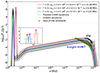 |
Fig. 1. Observed peak frequencies and corresponding peak flux densities of FRB 20200428 (stars) and the spectra of potentially associated X-ray bursts from SGR 1935+2154 observed with Insight-HXMT (green and orange bow ties) and KW (black data points) together with our model analysis results. The gray lines represent the model-predicted spectra of both FRB and associated X-ray bursts derived from 100 randomly selected model parameter sets based on our Monte Carlosimulation analysis and assuming |

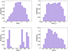 |
Fig. 2. Probability histograms of Γ, σ, γe, s, and νP derived from our simulation analysis. |
We calculated the plasma synchrotron maser and synchrotron emission of the electrons in an individual plasma blob. Through a Monte Carlo simulation analysis, we sampled model parameter sets of {Γ, γe, s, σ, νP}, which can produce observable FRB outbursts with CHIME and STARE2, and their associated X-ray bursts from SGR 1935+2154 with Insight-HXMT and KW. Following Li et al. (2025), the size of the individual blob in the comoving frame was estimated as Δ = Γcδt = 3 × 10⁷Γ cm, assuming δt = 1 ms, where c is the light speed. The luminosity distance to SGR 1935+2154 is estimated to be in the range 6.6–12.5 kpc (Kothes et al. 2018; Zhou et al. 2020; Zhong et al. 2020). We set a fiducial value of 10 kpc (z ∼ 0). The procedure of our Monte Carlo simulation is described below.
-
We fixed the νpk value at 0.475, 0.64, or 1.37 GHz, as observed by CHIME and STARE2, and generated a set of {Γ, γe, s, σ} values assuming that they are uniformly distributed in the ranges Γ ∈ [1, 200], γe, s ∈ [103, 105], and
 . The distribution range of σ was derived from the weak magnetization condition (γe, s2 > σ−1/2 > 1).
 -
We calculated the plasma synchrotron maser emission of the electrons in the blob. We first calculated the νP value with Eq. (11) for the case of γe, s2σ1/2 > 50 (Li et al. 2025), and then calculated the simulated peak flux density (Fνpksim) at νpk with Eq. (10) for the parameter set of {Γ, γe, s, σ, νP}. We checked whether the Fνpksim value is in the range
 MJy, as observed with CHIME and STARE2. If it was, we moved on the next step. Otherwise, we went back to Step 1.
 -
We calculated the peak frequency of the synchrotron emission of the electrons in an attempt to explain the associated X-ray bursts with ν = 0.45Γ2γe, s3νB and calculated corresponding flux density (Fν) using Eq. (10). We checked whether ν ∈ [2, 8]×1018 GHz and Fν ∈ [10−3, 10−1.5] Jy, as observed with Insight-HXMT and KW. If they were, the parameter set was selected as one possible model parameter set. Otherwise, we discarded this parameter set and repeated the above steps.
We repeated this procedure to generate a sample of 5000 sets of model parameters. We show their probability histograms in Fig. 2. The probability distribution of Γ is found to typically range from 5 to 30 with a median of 13. The probability distribution of γe, s is uniformly distributed in the range 1.8 × 10⁴ − 3.3 × 10⁴. The distribution of σ has three separated peaks, at  , which correspond to the three observed FRB outbursts with different νpk values. The distribution of νP ranges from log νP = 6.40 (νP = 2.48 MHz) to log νP = 7.6 (νP = 42.61 MHz).
We randomly selected 100 sets of model parameters from the 5000 sets and illustrate the spectra derived from our model for these 100 in Fig. 1. The predicted FRB outbursts and their associated X-ray bursts are detectable. By further fine-tuning the parameters as {Γ, γe, s, σ, νP/MHz}={15, 2.4 × 10⁴, 6.4 × 10⁻⁵, 11.68},{15, 2.4 × 10⁴, 13.3 × 10⁻⁵, 6.48}, and {15, 2.4 × 10⁴, 17.9 × 10⁻⁵, 5.23}, we obtain νpk = 1.37, 0.63, 0.47 GHz and Fνpk = 2.5, 0.15, 0.11 MJy, as shown by the solid red, blue, and green lines in Fig. 1. The predicted spectra closely fit the three observed FRB 20200428 bursts and potentially associated X-ray bursts. The synchrotron emission of the electrons is in the range 1010 ∼ 1020 Hz. It peaks around the hard X-ray band, with a flux density of 10−5 ∼ 10−2 Jy.
4. Discussion
An electron population with an energy distribution steeper than γe2 is required to generate plasma maser radiations. Schlickeiser (1984) developed an evolutionary model for relativistic electron energy spectra based on Fermi acceleration at shock fronts, second-order Fermi acceleration due to moving magnetized fluid elements, and energy losses due to synchrotron and inverse Compton radiation. Regardless of the injection spectrum of the particles, the energy distribution of the accelerated particles exhibits a power law form with a peak at γe, s, where γe, s corresponds to the point at which the Fermi acceleration timescale equals the radiation loss timescale. The spectral index of the power law below γe, s is determined by the ratio of the acceleration timescale to the particle escape lifetime. In the case of a very long escape lifetime, particles pile up sharply around γe, s, and the spectrum exhibits an exponential cutoff beyond γe, s, resulting in an almost monoenergetic particle distribution. In addition, collisionless shocks can result in a nonthermal component with  in the high-energy regime, and a thermal component with γe2 in the low-energy regime (Rybicki & Lightman 1986; Spitkovsky 2008). These two components are joined at γe, s. As nonthermal electrons cool radiatively, they gradually lose energy and accumulate at lower energies near γe, s, forming a very narrow distribution at γe, s (Sagiv & Waxman 2002). Therefore, in our calculations of plasma maser emission, we simply approximated the electron distribution as a monoenergetic population.
The peak flux density of plasma maser emission is sensitive to the σ and νP of a plasma blob. Figure 3 shows the spectra of the plasma maser emission and synchrotron emission when adopting different sets of σ and νP values. One can observe that the peak flux density of the maser emission varies by more than 10 orders of magnitude, while the flux density of the synchrotron emission only varies by 1–2 orders of magnitude. This presents a potential explanation for the observed sub-energetic radio bursts or giant radio pulses from SGR 1935+2154. We note that follow-up observations of SGR 1935+2154 detected several bright radio bursts with peak flux densities ranging from 1.8 Jy to 3.8 kJy (Kirsten et al. 2021; Giri et al. 2023). One of them was detected simultaneously with a short X-ray burst observed by the Gravitational-wave high-energy electromagnetic counterpart all-sky monitor (GECAM), Insight-HXMT high-energy burst searcher (HEBS), and KW. This is consistent with our model prediction.
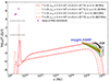 |
Fig. 3. Same as Fig. 1 but the model parameters are varied, as marked in the panel, to illustrate a possible explanation for the observed sub-energetic radio bursts or giant radio pulses from SGR 1935+2154. The dashed black lines indicate the range of several bright radio bursts detected in follow-up observations of SGR 1935+2154. |
The size and location of the radiating blobs are of interest. Based on the derived parameter sets from our Monte Carlo simulation analysis, we inferred the size of the blobs to be ∼109 − 10 cm and the magnetic field of the plasma blobs to be B = 102 ∼ 0.7 × 10⁴ G. Assuming that FRBs are powered by the magnetic energy of a magnetar (Lyubarsky 2014), we estimated the location of the FRB radiating blob to be rFRB ∼ bBpRp/B, where Rp is the radius of the magnetar and b (< 1) is a dimensionless constant. SGR 1935+2154 has a spin period of P ≃ 3.24 s, a spin-down rate of Ṗ ≃ 1.43 × 10⁻¹¹ s s−1, and a surface dipole magnetic field strength of Bp ≃ 2.2 × 10¹⁴ G (Gaensler 2014; Israel et al. 2016). We estimated the value of b as b ∼ (EXRB/EB)1/2 (Margalit et al. 2020), where EB is the total magnetic energy of SGR 1935+2154 and EXRB is the released energy of the two narrow X-ray peak bursts (which lasted 4 ms) associated with FRB 20200428. We have  erg. The value of EXRB for the hard X-ray peak bursts from SGR 1935+2154 is ∼1038 erg (Ridnaia et al. 2021). Thus, we have b ∼ 10−4. We obtain rFRB = 3.1 × 10¹² ∼ 2.2 × 1014 cm, which suggests that the sites of the FRB bursts are far from the central engine. This is evidence in support of the “far-away” scenarios (Lu et al. 2020; Margalit et al. 2020; Yu et al. 2021).
It should also be noted that the fitting results shown in Fig. 1 correspond to the time-integrated spectrum of the ∼1 s X-ray data observed by Insight-HXMT during the FRB 20200428 burst (Li et al. 2021), as well as the X-ray data with a duration of ∼0.46 s observed by KW (Ridnaia et al. 2021). However, this comparison is reasonable because the hardness of the light curve of the X-ray burst reaches its maximum at the location of the two narrow peaks and lasts ∼1 ms. This means that the two narrow peaks must be dominated by a nonthermal spectrum (Li et al. 2021; Ridnaia et al. 2021). In addition, the non-detection of radio emission from about one hundred typical soft bursts of SGR 1935+2154 further supports the idea that magnetar FRB signals are associated with rare X-ray bursts with hard spectra (Lin et al. 2020).
5. Conclusions
We have demonstrated that the observed flux densities and spectra of both FRB 20200428 and two potentially associated narrow X-ray peak bursts from SGR 1935+2154 can be explained using our model, which attributes the FRB and the X-ray bursts to plasma synchrotron maser emission and synchrotron radiation from weakly magnetized relativistic plasma blobs, respectively. We performed a Monte Carlo simulation analysis to constrain the model parameters that can generate observable FRB outbursts and potential X-ray bursts. It is found that Γ is in the range 5–30. The γe, s is uniformly distributed in the range 1.8 × 10⁴ − 3.3 × 10⁴. The distribution of σ exhibits three separated peaks, at log(σ) = {−4.21,−3.95,−3.88}, corresponding to the three detected bursts of FRB 20200428. The distribution of νP ranges from log νP = 6.40 (νP = 2.48 MHz) to log νP = 7.6 (νP = 42.61 MHz). The inferred size of the blobs is ∼109 − 10 cm, and the blob is located ∼1012 − 14 cm from the central engine. Adopting fine-tuned parameter sets as {Γ, γe, s, σ, νP/MHz}={15, 2.4 × 10⁴, 6.4 × 10⁻⁵, 11.68},{15, 2.4 × 10⁴, 13.3 × 10⁻⁵, 6.48}, and {15, 2.4 × 10⁴, 17.9 × 10⁻⁵, 5.23}, the observed spectra of both FRB 20200428 and the X-ray bursts from SGR 1935+2154 can indeed be reproduced by our model. Furthermore, the peak flux density of plasma maser emission is sensitive to σ and νP. It can vary by over 10 orders of magnitude, whereas the synchrotron emission flux density only varies by 1–2 orders of magnitude, consistent with the observed sub-energetic radio bursts or giant radio pulses from SGR 1935+2154.
As illustrated in Fig. 1, the synchrotron emission spectrum of plasma blobs is in the range 1010 to ∼1018 Hz. This suggests that short-duration optical and X-ray flashes can be accompanied by FRB bursts. Recently, an extragalactic FRB source, FRB 20250316A, was reported to be possibly associated with the X-ray source EP J120944.2+585060 detected by the Einstein Probe (Sun et al. 2025a). However, follow-up observations with the Chandra X-ray telescope did not support this association (Sun et al. 2025b). FRB 20250316A is a bright FRB from the nearby galaxy NGC 4141 and is located at a distance of ∼40 Mpc (Ng & CHIME/FRB Collaboration 2025). The nearest known extragalactic FRB is FRB 20200120E, which is located in a globular cluster of the M81 galaxy at a distance of ∼3.6 Mpc (Bhardwaj et al. 2021; Kirsten et al. 2022; Zhang et al. 2024). In contrast, typical FRBs are found at distances of ∼1 Gpc. If FRB 20200428 had occurred at a distance of 10 Mpc, its radio flux density would be ∼1 Jy ( ), while the X-ray and multiwavelength counterpart would be too faint to be detectable. Searching for associated X-ray/optical counterparts of cosmic FRBs is challenging with current time-domain astronomy.
One may have doubts as to whether the bursts detected by the two telescopes are the same event. We note that the spectrum of the second burst of FRB 20200428 detected by CHIME is narrowly banded and can be fitted with a Gaussian function (Chime/Frb Collaboration 2020). However, the spectrum observed by STARE2 cuts off at ∼1.29 GHz (see Fig. 1 in Bochenek et al. 2020). Therefore, the spectrum observed by CHIME should not be an extension of the burst detected by STARE2 since STARE2 covers a frequency range of 1.28–1.47 GHz but CHIME covers 0.4–0.8 GHz. In addition, the burst detected by CHIME lasts 0.335 ms, whereas the burst detected by STARE2 has a temporal width of 0.61 ms (Chime/Frb Collaboration 2020; Bochenek et al. 2020). Thus, the bursts detected by the two telescopes are likely two separate events from two blobs.
Acknowledgments
We thank the anonymous referee for helpful comments. We thank the helpful discussions with Shu-Qing Zhong, Hao-Hao Chen and Ying Gu. This work is supported by the National Key R&D Program (2024YFA1611700) and the National Natural Science Foundation of China (grant Nos. 12133003). E. W. L. is supported by the Guangxi Talent Program (“Highland of Innovation Talents”).
References
- Aleksandrov, A. F., Bogdankevich, L. S., & Rukhadze, A. A. 1984, Principles of Plasma Electrodynamics, 9, 2444 [Google Scholar]
- Beloborodov, A. M. 2017, ApJ, 843, L26 [NASA ADS] [CrossRef] [Google Scholar]
- Beloborodov, A. M. 2020, ApJ, 896, 142 [NASA ADS] [CrossRef] [Google Scholar]
- Bhandari, S., Heintz, K. E., Aggarwal, K., et al. 2022, AJ, 163, 69 [NASA ADS] [CrossRef] [Google Scholar]
- Bhardwaj, M., Gaensler, B. M., Kaspi, V. M., et al. 2021, ApJ, 910, L18 [NASA ADS] [CrossRef] [Google Scholar]
- Bochenek, C. D., Ravi, V., Belov, K. V., et al. 2020, Nature, 587, 59 [NASA ADS] [CrossRef] [Google Scholar]
- CHIME/FRB Collaboration (Andersen, B. C., et al.) 2020, Nature, 587, 54 [Google Scholar]
- Chime/Frb Collaboration (Amiri, M., et al.) 2020, Nature, 582, 351 [NASA ADS] [CrossRef] [Google Scholar]
- CHIME/FRB Collaboration (Amiri, M., et al.) 2021, ApJS, 257, 59 [NASA ADS] [CrossRef] [Google Scholar]
- Chime/Frb Collaboration (Andersen, B. C., et al.) 2023, ApJ, 947, 83 [NASA ADS] [CrossRef] [Google Scholar]
- Cordes, J. M., & Chatterjee, S. 2019, ARA&A, 57, 417 [NASA ADS] [CrossRef] [Google Scholar]
- Dai, Z. G. 2020, ApJ, 897, L40 [NASA ADS] [CrossRef] [Google Scholar]
- Fonseca, E., Andersen, B. C., Bhardwaj, M., et al. 2020, ApJ, 891, L6 [NASA ADS] [CrossRef] [Google Scholar]
- Gaensler, B. M. 2014, GCN, 16533, 1 [Google Scholar]
- Geng, J.-J., Li, B., Li, L.-B., et al. 2020, ApJ, 898, L55 [NASA ADS] [CrossRef] [Google Scholar]
- Ginzburg, V. L. 1989, Applications of Electrodynamics in Theoretical Physics and Astrophysics (New York: Gordon and Breach) [Google Scholar]
- Giri, U., Andersen, B. C., Chawla, P., et al. 2023, ApJ, submitted [arXiv:2310.16932] [Google Scholar]
- Gruzinov, A., & Waxman, E. 2019, ApJ, 875, 126 [NASA ADS] [Google Scholar]
- Heintz, K. E., Prochaska, J. X., Simha, S., et al. 2020, ApJ, 903, 152 [NASA ADS] [CrossRef] [Google Scholar]
- Israel, G. L., Esposito, P., Rea, N., et al. 2016, MNRAS, 457, 3448 [NASA ADS] [CrossRef] [Google Scholar]
- Katz, J. I. 2014, Phys. Rev. D, 89, 103009 [NASA ADS] [CrossRef] [Google Scholar]
- Kirsten, F., Snelders, M. P., Jenkins, M., et al. 2021, Nat. Astron., 5, 414 [Google Scholar]
- Kirsten, F., Marcote, B., Nimmo, K., et al. 2022, Nature, 602, 585 [NASA ADS] [CrossRef] [Google Scholar]
- Kothes, R., Sun, X., Gaensler, B., & Reich, W. 2018, ApJ, 852, 54 [NASA ADS] [CrossRef] [Google Scholar]
- Kumar, P., Lu, W., & Bhattacharya, M. 2017, MNRAS, 468, 2726 [NASA ADS] [CrossRef] [Google Scholar]
- Li, C. K., Lin, L., Xiong, S. L., et al. 2021, Nat. Astron., 5, 378 [NASA ADS] [CrossRef] [Google Scholar]
- Li, X., Lyu, F., Zhang, H. M., Deng, C.-M., & Liang, E.-W. 2025, A&A, 695, A100 [NASA ADS] [CrossRef] [EDP Sciences] [Google Scholar]
- Lin, L., Zhang, C. F., Wang, P., et al. 2020, Nature, 587, 63 [Google Scholar]
- Liu, Z.-N., Geng, J.-J., Yang, Y.-P., et al. 2023, ApJ, 958, 35 [NASA ADS] [CrossRef] [Google Scholar]
- Lorimer, D. R., Bailes, M., McLaughlin, M. A., Narkevic, D. J., & Crawford, F. 2007, Science, 318, 777 [Google Scholar]
- Lu, W., Kumar, P., & Zhang, B. 2020, MNRAS, 498, 1397 [NASA ADS] [CrossRef] [Google Scholar]
- Lyubarsky, Y. 2014, MNRAS, 442, L9 [Google Scholar]
- Lyubarsky, Y. 2021, Universe, 7, 56 [NASA ADS] [CrossRef] [Google Scholar]
- Margalit, B., & Metzger, B. D. 2018, ApJ, 868, L4 [NASA ADS] [CrossRef] [Google Scholar]
- Margalit, B., Beniamini, P., Sridhar, N., & Metzger, B. D. 2020, ApJ, 899, L27 [NASA ADS] [CrossRef] [Google Scholar]
- Mereghetti, S., Savchenko, V., Ferrigno, C., et al. 2020, ApJ, 898, L29 [Google Scholar]
- Metzger, B. D., Margalit, B., & Sironi, L. 2019, MNRAS, 485, 4091 [NASA ADS] [CrossRef] [Google Scholar]
- Ng, M.& CHIME/FRB Collaboration 2025, ATel, 17081, 1 [Google Scholar]
- Petroff, E., Barr, E. D., Jameson, A., et al. 2016, PASA, 33, e045 [NASA ADS] [CrossRef] [Google Scholar]
- Petroff, E., Hessels, J. W. T., & Lorimer, D. R. 2022, A&ARv, 30, 2 [NASA ADS] [CrossRef] [Google Scholar]
- Planck Collaboration XIII. 2016, A&A, 594, A13 [NASA ADS] [CrossRef] [EDP Sciences] [Google Scholar]
- Platts, E., Weltman, A., Walters, A., et al. 2019, Phys. Rep., 821, 1 [NASA ADS] [CrossRef] [Google Scholar]
- Qu, Y., & Zhang, B. 2024, ApJ, 972, 124 [Google Scholar]
- Ridnaia, A., Svinkin, D., Frederiks, D., et al. 2021, Nat. Astron., 5, 372 [NASA ADS] [CrossRef] [Google Scholar]
- Rybicki, G. B., & Lightman, A. P. 1986, Radiative Processes in Astrophysics (Wiley-VCH) [Google Scholar]
- Sagiv, A., & Waxman, E. 2002, ApJ, 574, 861 [NASA ADS] [CrossRef] [Google Scholar]
- Schlickeiser, R. 1984, A&A, 136, 227 [NASA ADS] [Google Scholar]
- Spitkovsky, A. 2008, ApJ, 682, L5 [NASA ADS] [CrossRef] [Google Scholar]
- Sun, H., Cheng, H. Q., Li, D. Y., et al. 2025a, ATel, 17100, 1 [Google Scholar]
- Sun, H., Li, D. Y., Jin, C. C., et al. 2025b, ATel, 17119, 1 [Google Scholar]
- Tavani, M., Casentini, C., Ursi, A., et al. 2021, Nat. Astron., 5, 401 [NASA ADS] [CrossRef] [Google Scholar]
- Wang, W.-Y., Xu, R., & Chen, X. 2020, ApJ, 899, 109 [Google Scholar]
- Waxman, E. 2017, ApJ, 842, 34 [NASA ADS] [CrossRef] [Google Scholar]
- Wu, Q., Zhang, G. Q., Wang, F. Y., & Dai, Z. G. 2020, ApJ, 900, L26 [Google Scholar]
- Xiao, D., & Dai, Z.-G. 2020, ApJ, 904, L5 [NASA ADS] [CrossRef] [Google Scholar]
- Xiao, D., Wang, F., & Dai, Z. 2021, Sci. China: Phys. Mech. Astron., 64, 249501 [Google Scholar]
- Yang, Y.-P., & Zhang, B. 2018, ApJ, 868, 31 [NASA ADS] [CrossRef] [Google Scholar]
- Yang, Y.-P., Zhu, J.-P., Zhang, B., & Wu, X.-F. 2020, ApJ, 901, L13 [NASA ADS] [CrossRef] [Google Scholar]
- Yu, Y.-W., Zou, Y.-C., Dai, Z.-G., & Yu, W.-F. 2021, MNRAS, 500, 2704 [Google Scholar]
- Zhang, B. 2020, Nature, 587, 45 [CrossRef] [Google Scholar]
- Zhang, B. 2022, ApJ, 925, 53 [NASA ADS] [CrossRef] [Google Scholar]
- Zhang, B. 2023, Rev. Mod. Phys., 95, 035005 [NASA ADS] [CrossRef] [Google Scholar]
- Zhang, S. B., Wang, J. S., Yang, X., et al. 2024, Nat. Commun., 15, 7454 [Google Scholar]
- Zhong, S.-Q., Dai, Z.-G., Zhang, H.-M., & Deng, C.-M. 2020, ApJ, 898, L5 [NASA ADS] [CrossRef] [Google Scholar]
- Zhou, P., Zhou, X., Chen, Y., et al. 2020, ApJ, 905, 99 [NASA ADS] [CrossRef] [Google Scholar]
All Figures
|
Fig. 1. Observed peak frequencies and corresponding peak flux densities of FRB 20200428 (stars) and the spectra of potentially associated X-ray bursts from SGR 1935+2154 observed with Insight-HXMT (green and orange bow ties) and KW (black data points) together with our model analysis results. The gray lines represent the model-predicted spectra of both FRB and associated X-ray bursts derived from 100 randomly selected model parameter sets based on our Monte Carlosimulation analysis and assuming |
| In the text | |
|
Fig. 2. Probability histograms of Γ, σ, γe, s, and νP derived from our simulation analysis. |
| In the text | |
|
Fig. 3. Same as Fig. 1 but the model parameters are varied, as marked in the panel, to illustrate a possible explanation for the observed sub-energetic radio bursts or giant radio pulses from SGR 1935+2154. The dashed black lines indicate the range of several bright radio bursts detected in follow-up observations of SGR 1935+2154. |
| In the text | |
Current usage metrics show cumulative count of Article Views (full-text article views including HTML views, PDF and ePub downloads, according to the available data) and Abstracts Views on Vision4Press platform.
Data correspond to usage on the plateform after 2015. The current usage metrics is available 48-96 hours after online publication and is updated daily on week days.
Initial download of the metrics may take a while.