| Issue |
A&A
Volume 702, October 2025
|
|
|---|---|---|
| Article Number | A45 | |
| Number of page(s) | 15 | |
| Section | Planets, planetary systems, and small bodies | |
| DOI | https://doi.org/10.1051/0004-6361/202555284 | |
| Published online | 07 October 2025 | |
Exploring the formation of multiple dust-trapping rings in the inner Solar System
1
Université Côte d’Azur, Observatoire de la Côte d’Azur, CNRS,
Laboratoire Lagrange,
France
2
Collège de France,
11 Pl. Berthelot,
75005
Paris,
France
3
Instituto de Ciencias Físicas, Universidad Nacional Autónoma de México, Av. Universidad s/n,
62210
Cuernavaca, Mor.,
Mexico
4
DPHY, ONERA, Université Paris Saclay,
91120
Palaiseau,
France
★ Corresponding author.
Received:
24
April
2025
Accepted:
30
July
2025
Abstract
Context. Isotopic properties of meteorites provide evidence that multiple dust trap or pressure bumps had to form and persist in the inner Solar System on a timescale of millions of years. The formation of a pressure bump at the outer edge of the gap opened by Jupiter would be effective in blocking particles drifting from the outer to the inner disc. Yet this would not be enough to preserve dust in the inner disc. However, in low-viscosity discs and under specific conditions governing the gas cooling time, it has been shown that massive planets can also open secondary gaps, separated by density bumps, inwards of the main gap. The majority of studies of the process of secondary gap formation have been done in two dimensional equatorial simulations with prescribed disc cooling or by approximating the cooling from the disc photosphere. Recent results have shown that an appropriate computation of the disc cooling by including the treatment of radiation transport is key to determining the formation of secondary gaps.
Aims. Our aim is to extend previous studies to three dimensional discs by also including radiative effects. Moreover, we also consider non-ideal magnetohydrodynamic effects in discs with a prescribed cooling time to explore the feedback of the magnetic field on secondary gap formation.
Methods. We performed three dimensional hydrodynamical numerical simulations with a self-consistent treatment of radiative effects making use of a flux-limited diffusion approximation. We then extended our study to a similar disc including the magnetic field and non-ideal Ohmic and ambipolar effects.
Results. We show that in the hydrodynamical model, a disc with low bulk viscosity (αν = 10−4) and consistent treatment of radiative effects, a Jupiter-mass planet is capable of opening multiple gaps. We also show that multiple gaps and rings are formed by planetary masses close to the pebble isolation mass. In the presence of non-ideal MHD effects, multiple gaps and rings are also formed by a Jupiter-mass planet.
Conclusions. A solid Jupiter core in low-viscosity discs blocks particles drifting towards and within the inner disc. The formation of multiple gaps and rings inside the planetary orbit at this stage is crucial to preserving dust reservoirs. Such reservoirs are pushed towards the inner part of the disc during Jupiter runaway growth and they are shown to be persistent after Jupiter’s growth. Multiple dust reservoirs could therefore be present in the inner Solar System since the formation of Jupiter’s solid core when the disc is characterised by low viscosity.
Key words: accretion, accretion disks / hydrodynamics / magnetohydrodynamics (MHD) / protoplanetary disks / planet-disk interactions
© The Authors 2025
 Open Access article, published by EDP Sciences, under the terms of the Creative Commons Attribution License (https://creativecommons.org/licenses/by/4.0), which permits unrestricted use, distribution, and reproduction in any medium, provided the original work is properly cited.
This article is published in open access under the Subscribe to Open model. This email address is being protected from spambots. You need JavaScript enabled to view it. to support open access publication.
1 Introduction
Meteorites are divided into two broad categories: chondrites and achondrites (with iron meteorites included in the latter). The parent bodies of achondrites formed in the first megayear (Myr) of the Solar System’s existence. They contained a large abundance of short-lived radioactive elements, whose decay liberated enough energy to melt these bodies (Neumann et al. 2012). Under the effect of gravity, these bodies then differentiated into an iron core, a silicate mantle and a crust, akin to the structure of asteroid 4 Vesta. The parent bodies of chondrites formed later, so that most short-lived radioactive atoms had already decayed. Consequently, the energy liberated in their interior was not as high; temperatures increased significantly, up to several hundred degrees, but not enough to cause melting. Thus, these bodies preserved their original petrological structure, made of chondrules and matrix and refractory inclusions. From measurements of the ages of formation of the individual chondrules, the chondrite parent bodies formed approximately 2–4 My after the beginning of the Solar System (Fukuda et al. 2022; Piralla et al. 2023). The formation of planetesimals so late in the history of the protoplanetary disc is problematic, because dust particles (i.e. the individual chondrules, or the matrix grain aggregates) tend to drift radially towards to Sun on a timescale that is much shorter than a million years. We might consider that the dust lost by radial drift at a given location was substituted by dust drifting from larger radial distances in the disc; however, this simple view is negated by another crucial observation in meteorite science. The analysis of nucleosynthetic isotopic anomalies inherited from the interstellar medium reveals that both chondrites and achondrites are distinguished into two distinct groups, dubbed CC – as the measured anomalies are like those of carbonaceous chondrites – and NC – as the anomalies are like those of non-carbonaceous chondrites (Warren 2011; Kruijer et al. 2017). The existence of an isotopic dichotomy such as that described above implies that the objects of the NC and CC groups formed at different locations of the disc, incorporating distinct materials. Because CCs exhibit evidence of prominent water alteration, whereas the isotopic properties of NC meteorites are similar to those of Earth and Mars, the common interpretation is that the NC bodies (both achondrites and chondrites) formed in the inner Solar System and the CC bodies (again both achondrites and chondrites) formed in the outer Solar System, where water could be accreted in solid form (Kruijer et al. 2017; Nanne et al. 2019). An implication of these considerations is that the material that formed the NC chondrites in the inner Solar System at a later time could not have drifted from the outer disc; otherwise it would have exhibited CC isotopic properties. The formation of Jupiter, opening a gap in the disc (Kruijer et al. 2017), or the formation of a pressure bump near the snowline (Brasser & Mojzsis 2020) must have blocked the drift of particles from the outer disc to the inner disc. Again, meteorites provide evidence that only particles smaller than 200 microns could pass through such dynamical barriers, with negligible effect on the overall mass balance (Haugbølle et al. 2019).
Thus, in the absence of a refilling mechanism, the NC dust in the inner part of the protoplanetary disc had to survive for millions of years without drifting into the Sun. This would require the existence of a pressure bump in the disc where dust could be trapped. A pressure bump may be generated near 1 au if the disc evolves primarily under the effects of magnetised winds and if the mass removal rate in these winds increases with decreasing heliocentric distance (Suzuki et al. 2010; Ogihara et al. 2018). The existence of a unique pressure bump, however, is not completely satisfactory (Kleine et al. 2020; Schneider et al. 2020). Four kinds of NC chondrites exist, with somewhat different isotopic anomalies: the prominent ordinary and enstatite chondrite groups, followed by the Rumuruti (R) and Kakangari (K) groups, which are represented to a lesser extent in the meteorite collections. Together with the fact that Enstatite chondrites have essentially identical isotopic properties of a class of NC achondrites called Aubrites, this implies that the dust did not get completely mixed up, even on a timescale of millions of years. This strongly suggests that it was not one, but several pressure bumps, which had to form and persist in the inner part of the protosolar disc.
Multiple rings of dust are observed in protoplanetary discs (Andrews et al. 2018), suggestive of a multitude of pressure bumps. A long-debated question is whether the formation of these pressure bumps is due to the formation of massive planets opening gaps in the disc (Bae et al. 2017) or to spontaneous non-ideal magnetohydrodynamic (MHD) effects (Béthune et al. 2017; Riols & Lesur 2018; Cui & Bai 2021). We remark that spontaneous generation of rings has been obtained (by Béthune et al. 2017; Riols & Lesur 2018; Cui & Bai 2021) in cases where ampipolar diffusion is the dominant non-ideal effect. This result suggests that such rings would not not form in the inner disc because the MHD dynamics there is thought to be dominated by Hall and Ohmic dissipation, rather than ambipolar diffusion (Armitage 2011).
The rings are observed only in the outer part of protoplanetary discs and, due to resolution effects, it is not possible to assess observationally whether they are common also in the inner part. Also, none of the terrestrial planets was massive enough to open a gap in the disc, even if already present with its current mass, because their Hill sphere is much smaller than the vertical scale height of the disc. Therefore, Jupiter remains the main suspect for the potential formation of rings in the inner disc. Jupiter obviously forms a prominent pressure bump outside of the main gap that opens along its orbit, but this is of no help with respect to the preservation of dust in the inner system. It has been shown, however, that massive planets can also open secondary gaps, separated by density bumps, also inwards of the main gap (Bae et al. 2016, 2017; Miranda & Rafikov 2020a).
Most studies of the process of secondary gap formation have been conducted in 2D equatorial simulations (Bae et al. 2017; Zhang et al. 2018; Miranda & Rafikov 2019, 2020a; Ziampras et al. 2023) and show that three necessary conditions have to be met: (i) the disc must have a very small effective turbulent viscosity; (ii) the disc cooling time normalised by the local orbital frequency, denoted βc, has to be either small (βc < 0.01) or large (βc > 10) (Miranda & Rafikov 2020a; Ziampras et al. 2023); and (iii) the planet must be massive enough (with the mass depending on the disc’s viscosity, βc, and on the disc’s scale height.
Including a prescription of radiative effects gives the appropriate cooling time associated to disc properties and is a necessary step in capturing the dynamics of the formation of secondary gaps in specific discs. Taking into account the cooling from the disc surface (Ziampras et al. 2020) and adding radiation transport along the disc midplane (Miranda & Rafikov 2020a; Ziampras et al. 2023) have improved the treatment of disc thermodynamics in 2D simulations. However, a self-consistent treatment of radiative effects in 3D simulations of secondary gap opening has not yet been considered. To our knowledge, the only 3D simulations with an appropriate βc from disc surface irradiation and a Jupiter-mass planet in a massive, inviscid protoplanetary disc were presented in Bae et al. (2016). This work indicated several waves in the disc’s surface density distribution inwards of Jupiter’s orbit. The authors, however, did not perform an analysis of the pressure profile in the disc to verify whether dust-trapping pressure bumps formed.
Given the relevance of this problem to understand the formation of different classes of NC chondrites, we present an exploration of the capability of Jupiter to form multiple dust-trapping rings in the inner Solar System using a self-consistent treatment of radiative effects in a disc with low bulk viscosity. Moreover, since low-viscosity discs transport gas towards the star at a very low rate with respect to typical accretion rates observed in young stars (Hartmann et al. 1998; Manara et al. 2016), we decided to extend our model by including non-ideal MHD effects. In this case, accretion flow onto the star is obtained by angular momentum removal by disc winds (Béthune et al. 2017; Lesur 2021b) and our aim is to explore the feedback of the magnetic field on secondary gap formation.
The paper is organised as follows. In Section 2, we present our simulation tools and methods. In Section 3, we reproduce the work of Bae et al. (2016) and compute the pressure profile on the midplane. In Section 4, we present a different simulation, where we adopt a density comparable to the minimum mass solar nebula at the planet location, instead of the massive disc used by Bae et al. (2016). In addition, we compute βc self-consistently using flux-limited energy diffusion. In Section 5, we extend our model including non-ideal MHD effects. Finally, in Section 6, we progressively reduce the mass of the planet to see at which mass a planetary core might have started to form dust-trapping rings in the inner Solar System.
2 Models
2.1 Physical model
The protoplanetary disc (PPD hereafter) is treated as a non-self-gravitating gas whose motion is described by the Navier-Stokes equations. We used two grid-based codes: the fargOCA code (Lega et al. 2014), which integrates a full energy equation taking into account viscous heating and radiative cooling and the FARGO3D code (Benítez-Llambay & Masset 2016), which includes non-ideal MHD effects. The two codes are very similar in the sense that they use the same hydrodynamical solvers based on the operator splitting procedure (Stone et al. 1992) and they both benefit from the FARGO algorithm (Masset 2000) for a computation of the time step suited to gas rotating with quasi-Keplerian motion. The reason for the use of the two codes solely depends on the different physical modules that they implement.
In both cases, we used spherical coordinates (r, θ, φ), where r is the radial distance from the star (which is at the origin of the coordinate system), θ the polar angle measured from the z axis (the colatitude), and φ is the azimuthal coordinate measured from the x axis. The midplane of the disc is located at the equator, ![Mathematical equation: $\[\theta=\frac{\pi}{2}\]$](/articles/aa/full_html/2025/10/aa55284-25/aa55284-25-eq1.png) . We are working in a coordinate system that rotates with the angular velocity of a planet of mass, mp,
. We are working in a coordinate system that rotates with the angular velocity of a planet of mass, mp,
![Mathematical equation: $\[\Omega_k=\sqrt{\frac{G\left(M_{\star}+m_p\right)}{r_p{ }^3}},\]$](/articles/aa/full_html/2025/10/aa55284-25/aa55284-25-eq2.png)
where M⋆ is the mass of the central star, G is the gravitational constant, and rp is the semi-major axis of a planet assumed to be on a circular orbit. We consider a planet orbiting a Solar mass star and, therefore, in the following, we refer to the mass of the star as M⊙.
The dynamics of the gas is provided by the integration of the Navier-Stokes equations composed by a continuity equation and a set of three equations for the momenta (Lega et al. 2014; Benítez-Llambay & Masset 2016). Additionally, we consider the gas internal energy density as e = ρcvT, where ρ and T are the gas volume density and the gas temperature, while cv is the specific heat at constant volume. The equation of state is that of an ideal gas of pressure of P = (γ − 1)e with adiabatic index of γ = 1.4. In the following, we use either of two prescriptions for the integration of the energy equation:
-
Changes in the internal energy density e are due to adiabatic (de)compression, viscous heating, (Mihalas & Mihalas 1984) and a relaxation to the initial temperature, T0, on a cooling timescale of
![Mathematical equation: $\[\tau_{\mathrm{c}}=\beta_{c} \Omega_{k}^{-1}\]$](/articles/aa/full_html/2025/10/aa55284-25/aa55284-25-eq3.png) ,
,
![Mathematical equation: $\[\partial_t e+\nabla \cdot(e \mathbf{v})=-P \nabla \cdot \mathbf{v}+Q^{+}-\rho c_v \frac{\left(T-T_0\right)}{\tau_{\mathrm{c}}},\]$](/articles/aa/full_html/2025/10/aa55284-25/aa55284-25-eq4.png) (1)
(1)where v is the gas velocity, while the terms −P∇ · v and
![Mathematical equation: $\[Q^{+} \equiv \bar{\bar{\tau}} \nabla v\]$](/articles/aa/full_html/2025/10/aa55284-25/aa55284-25-eq5.png) are the compressional and viscous heating (
are the compressional and viscous heating (![Mathematical equation: $\[\bar{\bar{\tau}}\]$](/articles/aa/full_html/2025/10/aa55284-25/aa55284-25-eq6.png) is the viscous stress tensor defined in Mihalas & Mihalas 1984), respectively. The dimensionless cooling time βc is either a constant parameter or a function depending on disc properties, as described below.
is the viscous stress tensor defined in Mihalas & Mihalas 1984), respectively. The dimensionless cooling time βc is either a constant parameter or a function depending on disc properties, as described below. -
We consider the evolution of the internal energy and of the thermal radiation energy, Er (code fargOCA), in the flux-limited diffusion approximation (FLD, Levermore & Pomraning 1981) using the so-called two temperature approach (Commerçon et al. 2011), expressed as
![Mathematical equation: $\[\left\{\begin{array}{l}\partial_t E_{\mathrm{r}}-\nabla \cdot \boldsymbol{F}=\rho \kappa_p c\left(a_r T^4-E_{\mathrm{r}}\right), \\\partial_t e+\nabla \cdot(e \mathbf{v})=-P \nabla \cdot \boldsymbol{v}-\rho \kappa_p c\left(a_r T^4-E_{\mathrm{r}}\right)+Q^{+},\end{array}\right.\]$](/articles/aa/full_html/2025/10/aa55284-25/aa55284-25-eq7.png) (2)
(2)where
![Mathematical equation: $\[\boldsymbol{F}=\frac{c \lambda}{\rho \kappa_{r}} \nabla E_{\mathrm{r}}\]$](/articles/aa/full_html/2025/10/aa55284-25/aa55284-25-eq8.png) is the radiation flux vector and λ the flux limiter (Kley et al. 2009). We use κp and κr to indicate the Planck and the Rosseland mean opacity, respectively, with ar as the radiation constant and with c as the speed of light. In this paper, we consider κ = κp ≡ κr (see Bitsch et al. 2013) and use the opacity law of Bell & Lin (1994), where a dust to gas ratio of 0.01 is assumed.
is the radiation flux vector and λ the flux limiter (Kley et al. 2009). We use κp and κr to indicate the Planck and the Rosseland mean opacity, respectively, with ar as the radiation constant and with c as the speed of light. In this paper, we consider κ = κp ≡ κr (see Bitsch et al. 2013) and use the opacity law of Bell & Lin (1994), where a dust to gas ratio of 0.01 is assumed.We did not include the irradiation heating from the central star, so that we could reduce the computational cost with no significant impact on the gas dynamics in the planet vicinity (see Lega et al. 2015). However, we did consider low-viscosity disc with stellar irradiation as the main source of heating. Therefore, in our 3D simulations, we mimicked the thermal equilibrium structure obtained in discs heated by the star, by suitably fixing the disc surface temperature (see Section 4 and Lega et al. 2024). When considering the energy evolving according to Eq. (2), the disc cooling time, βc, fully depends on the disc properties and can be estimated a posteriori as explained below. In the following we refer to simulations as “fully radiative” with the above prescription for the energy computation.
2.2 Cooling time approximation
When computing an energy equation with temperature relaxing towards the initial values (Eq. (1)), it is customary to consider the cooling time, βc, as a constant parameter (see e.g. Miranda & Rafikov 2020b; Ziampras et al. 2023). However, when studying specific discs (or aiming to make comparisons to the observed disc structures), it is important to compute the cooling time from disc properties (Zhang et al. 2018; Miranda & Rafikov 2020a; Ziampras et al. 2023).
2.2.1 Cooling through disc surfaces
The cooling process occurs through blackbody emission of dust grains. In vertically integrated discs the radiative cooling power per unit surface is given by Menou & Goodman (2004), expressed as
![Mathematical equation: $\[Q_{cool}=-\frac{\sigma T^4}{\tau_{e f f}},\]$](/articles/aa/full_html/2025/10/aa55284-25/aa55284-25-eq9.png)
where σ = arc/4 and τeff is the effective optical depth (Hubeny 1990), expressed as
![Mathematical equation: $\[\tau_{e f f}=\frac{3}{8} \tau+\frac{\sqrt{3}}{4}+\frac{1}{4 \tau},\]$](/articles/aa/full_html/2025/10/aa55284-25/aa55284-25-eq10.png)
to take into account the optically thick and thin limits, while τ = 1/2κΣ is the optical depth at disc midplane.
The discs cools through surfaces and, following Ziampras et al. (2020) the surface cooling time can be written as
![Mathematical equation: $\[\beta_c^{surf}=\Omega_K \frac{\Sigma c_v T}{|2 Q_{cool|}} \equiv \Omega_K \frac{\Sigma c_v \tau_{e f f}}{2 \sigma T^3}.\]$](/articles/aa/full_html/2025/10/aa55284-25/aa55284-25-eq11.png) (3)
(3)
The formula has been extended to a three dimensional (3D) disc by Lyra et al. (2016) by considering the radiative timescale ![Mathematical equation: $\[t_{r}=\frac{e}{\nabla {\cdot} \boldsymbol{F}}\]$](/articles/aa/full_html/2025/10/aa55284-25/aa55284-25-eq12.png) (with e and F defined in Eq. (2)) and integrating over a spherical volume of radius, H1,
(with e and F defined in Eq. (2)) and integrating over a spherical volume of radius, H1,
![Mathematical equation: $\[\beta_c^H=\Omega_K \frac{\rho c_v H \tau_{e f f}}{3 \sigma T^3}.\]$](/articles/aa/full_html/2025/10/aa55284-25/aa55284-25-eq13.png) (4)
(4)
In this case, the optical depth τeff is computed for grid cells at height z above (below) the midplane as ![Mathematical equation: $\[\tau(z)=\int_{z}^{z_{max}} \rho(z^{\prime}) \kappa(z^{\prime}) \mathrm{d} z^{\prime} \left(\tau(z)=\int_{z_{min}}^{z} \rho(z^{\prime}) \kappa(z^{\prime}) \mathrm{d} z^{\prime}\right)\]$](/articles/aa/full_html/2025/10/aa55284-25/aa55284-25-eq14.png) .
.
2.2.2 In-plane cooling
Dust grains emission actually occurs in all directions, namely, the radiative flux has also a radial component in addition to the previously described surface cooling. A detailed study on the role of the radial radiative flux or in-plane cooling on the evaluation of the cooling timescale was performed by Miranda & Rafikov (2020a) and Ziampras et al. (2023) based on two-dimensional (2D) vertically integrated disc models. In those papers, an effective cooling time scale was obtained by combining the surface cooling of Eq. (3) and the in-plane cooling obtained considering heat diffusion through the mid-plane by Miranda & Rafikov (2020a). The results obtained underline the importance of considering the in-plane cooling component, suggesting that a study of 3D discs with heat diffusion from the FLD approximation is required to evaluate thermal processes and correctly estimate the cooling time, βc.
2.3 Cooling time in 3D discs with FLD approximation
When dealing with Eq. (2), heat diffusion is fully taken into account by computing the radiation flux on every grid-cell at any time, t. The cooling time can therefore be derived a posteriori from the timescale over which radiation is diffused over a typical length scale, lr,
![Mathematical equation: $\[\beta_c=\Omega_K \frac{l_r^2}{D_r},\]$](/articles/aa/full_html/2025/10/aa55284-25/aa55284-25-eq15.png) (5)
(5)
where Dr is the radiative diffusion coefficient of a grid cell at time, t. In the optically thick limit, the diffusion coefficient associated with the radiation flux vector in Eq. (2) is
![Mathematical equation: $\[D_r=\frac{16 \sigma T^3}{3 c_v \rho^2 \kappa},\]$](/articles/aa/full_html/2025/10/aa55284-25/aa55284-25-eq16.png) (6)
(6)
where we consider Er = arT4 and λ = 1/3. Although Eq. (5) overestimates the cooling time in the optically thin regions, we chose to keep this expression since typical discs are optically thick in the planet’s formation region near the midplane.
By considering the disc scale height, H, as the characteristic diffusion length scale, we obtain (see also Miranda & Rafikov 2020a; Ziampras et al. 2023) the following expression,
![Mathematical equation: $\[\beta_c=\Omega_K \frac{3 c_v \rho^2 \kappa H^2}{16 \sigma T^3}.\]$](/articles/aa/full_html/2025/10/aa55284-25/aa55284-25-eq17.png) (7)
(7)
We computed this quantity to compare the results obtained with the energy evolving with FLD approximation to those obtained with Eq. (1). We remark that the cooling time obtained from diffusion Eq. (7) in an optically thick disc is similar to the cooling from the disc’s photosphere, as given in Eqs. (3) and (4).
2.4 Non-ideal magnetic effects
To include MHD effects (with the code FARGO3D), we also considered the induction equation for the evolution of the magnetic field, B, as
![Mathematical equation: $\[\partial_t \boldsymbol{B}=\nabla \times\left(\boldsymbol{v} \times \boldsymbol{B}-\eta_O \boldsymbol{J}+\eta_A \boldsymbol{J} \times \boldsymbol{e}_b \times \boldsymbol{e}_b\right).\]$](/articles/aa/full_html/2025/10/aa55284-25/aa55284-25-eq18.png) (8)
(8)
With respect to the pure hydrodynamical case, the equation for the momenta have an additional source term, J × B (Benítez-Llambay & Masset 2016), where J ≡ ∇ × B is the electric current.
The terms ηO and ηA are the Ohmic and ambipolar diffusivities and eb is the unit vector parallel to the magnetic field line. We chose not to consider the Hall effect for the following reasons: (i) Ohmic resistivity is considered dominant in the region of interest near the midplane where the density is high; in addition, it was recently supposed that it is dominant even at low density values (Hopkins et al. 2024); (ii) to our knowledge, spiral arm propagation in MHD discs has not yet been investigated, so that we chose a relatively simple setting; (iii) finally, from the computational point of view, 3D MHD simulations with embedded planets are extremely expensive and Hall effect can contribute to further decreasing the time step that would make the integration of the system for about 100 planetary orbits prohibitive.
Following Lesur (2021b) and Wafflard-Fernandez & Lesur (2023), we prescribed the Ohmic and ambipolar profiles instead of considering a model for ionisation that would also make the 3D computations extremely expensive. We considered the dimensionless Ohmic Reynolds number, ℛO, and Elsasser number, ΛA, defined at disc midplane via
![Mathematical equation: $\[\Lambda_A(0) \equiv \frac{v_A^2}{\eta_A \Omega_k} \quad \mathcal{R}_O(0) \equiv \frac{\Omega_K H^2}{\eta_O},\]$](/articles/aa/full_html/2025/10/aa55284-25/aa55284-25-eq19.png)
where ![Mathematical equation: $\[v_{A}=B / \sqrt{\rho \mu_{0}}\]$](/articles/aa/full_html/2025/10/aa55284-25/aa55284-25-eq20.png) is the Alfvén velocity. According to Lesur (2021b) and Wafflard-Fernandez & Lesur (2023), we can consider the gas to be fully ionised in the corona. This is set via
is the Alfvén velocity. According to Lesur (2021b) and Wafflard-Fernandez & Lesur (2023), we can consider the gas to be fully ionised in the corona. This is set via
![Mathematical equation: $\[\begin{aligned}& \Lambda_A(z)=\max \left\{\Lambda_A(0) \exp \left[\frac{z^4}{(\xi H)^4}\right], \frac{1}{10} \frac{v_A^2}{c_s^2}\right\}, \\& \mathcal{R}_O(z)=\mathcal{R}_O(0) \exp \left[\frac{z^4}{(\xi H)^4}\right]\left(\frac{\rho(0)}{\rho(z)}\right),\end{aligned}\]$](/articles/aa/full_html/2025/10/aa55284-25/aa55284-25-eq21.png)
where ξ quantifies the thickness of the non-ideal layer in units of the pressure scale height H (ξ = 3 in our simulations).
We noticed that the models used to compute the Ohmic and ambipolar coefficients, while taking into account the ionisation of gas and chemical models (Gressel et al. 2015; Béthune et al. 2017; Bai 2017; Lesur 2021b,a), do not provide a clear consensus on the values of the strength of non-ideal effects. This is mainly due to a strong uncertainty about the ionisation rate from cosmic rays (the main source of ionisation below two scale heights) and on the size and abundance of grains in discs that tend to reduce the ionisation fraction.
In the simulations presented in Section 5, we considered ℛO = 1 and different values of ΛA ∈ [0.01 : 10]. This choice is motivated by the fact that values of RO ~ O(1) and strong (ΛA ~ 0.01) to weak ambipolar diffusion (ΛA ~ 10) are plausible (Gressel et al. 2015; Béthune et al. 2017; Bai 2017) in the region of the protoplanetary disc considered in this paper.
2.5 Disc models
The code units are such that G = M* ≡ M⊙ = 1 and the unit of distance r0 is arbitrary. The unit of time is therefore (r0/au)3/2/(2π) yr. For the simulations we adopt as the unit of length r0 = 5.2 au except for the MHD case for which r0 = 1 au. Planets are considered, in all cases, at a position of rp = 5.2 au. We call T0 the orbital period at r = r0. The simulations’ domain extend radially from rmin to rmax and vertically from the colatitude θ0 to the midplane at θ = π/2. We consider discs with radial profile of surface density Σ(r) = Σ0(r/r0)−αΣ. The values of these parameters as well as simulation names are reported in Table 1. The fully radiative simulations are named HDrad followed by J, S, and 30, for planets of respectively the mass of Jupiter, of Saturn, and of a super-Earth of 30 Earth masses. We considered non-zero α viscosity described by the parameter αν for the whole set of hydro-dynamical simulations – except HDBae. In the MHD simulations, angular momentum is transported by the magnetic field without the need to prescribe a viscosity (e.g. of turbulent origin).
Other parameters such as the boundary conditions and the numerical resolution do also depend on the simulation (specified in Table 2). In the azimuthal direction we use periodic boundary conditions. The label “damping” refers to the implementation of a wave damping region according to de Val-Borro et al. (2006). The radial grid spacing is logarithmic, the azimuthal one is constant, while the vertical spacing is constant except for the MHD simulations for which we use a nonuniform grid. The reason for this is attributed to magnetic effects, such as winds, developing on a large vertical domain and a non-uniform grid meeting the requirements of having a moderate total number of grid cells together with a suited resolution (~8 grid cells) over a disc scale height above the midplane. Precisely, our grid has constant resolution from the midplane up to one scale height and then it varies quadratically with a maximum resolution ratio of 4. Moreover, in the case of MHD simulations additional boundary conditions are required for the magnetic field and for the electromotive field (EMF). We report the details in Appendix C.
Disc model parameters.
Boundary conditions.
2.6 Discs with embedded planets: Numerical procedure
In all the simulations, we considered a planet on a fixed circular orbit located on the midplane at rp = 5.2 au (i.e. rp = r0 for all the simulations – except the MHD ones, for which rp = 5.2r0 with r0 = 1 au) and azimuth of φ = 0; or, equivalently, at (xp, yp, zp) = (5.2, 0, 0) au. We embedded in each disc model a planet of 20 Earth masses at t = 0 and smoothly increased this value over a time interval of 10 or 20 orbits until the mass until the final mass was reached. The fully radiative and MHD cases require preliminary 2D (r, θ) simulations to reach an equilibrium configuration prior to the planet insertion. This phase is described in the corresponding sections.
The gravitational potential of the planet acting on the disc (Φp) is modelled as in Kley et al. (2009) in the fargOCA code: the full gravitational potential is computed for disc elements having distance, d, from the planet larger than a fraction, ϵ, of the Hill radius, while it is smoothed for disc elements with d < rsm ≡ ϵRH according to
![Mathematical equation: $\[\Phi_p=\left\{\begin{array}{ll}-\frac{m_p G}{d} & d>r_{\mathrm{sm}} \\-\frac{m_p G}{d} f\left(\frac{d}{r_{\mathrm{sm}}}\right) & d \leq r_{\mathrm{sm}}\end{array},\right.\]$](/articles/aa/full_html/2025/10/aa55284-25/aa55284-25-eq23.png) (9)
(9)
with ![Mathematical equation: $\[f\left(\frac{d}{r_{\mathrm{sm}}}\right)=\left[\left(\frac{d}{r_{\mathrm{sm}}}\right)^{4}-2\left(\frac{d}{r_{\mathrm{sm}}}\right)^{3}+2 \frac{d}{r_{\mathrm{sm}}}\right]\]$](/articles/aa/full_html/2025/10/aa55284-25/aa55284-25-eq24.png) .
.
In FARGO3D the potential is smoothed according to
![Mathematical equation: $\[\Phi_p=-\frac{m_p G}{\sqrt{\left(d^2+r_{s m}^2\right)}}.\]$](/articles/aa/full_html/2025/10/aa55284-25/aa55284-25-eq25.png) (10)
(10)
We recall that the Hill radius is defined as: RH = rp(mp/3M⊙)1/3. The values of ϵ are respectively (0.13, 0.2, 0.1) in simulation sets (HDBae, HD,MHD).
3 Hydrodynamical case with prescribed cooling
The only 3D simulation, to our knowledge, which shows the formation of multiple rings and gaps inside the orbit of a Jupiter-mass planet is the one in Bae et al. (2016). This paper was mainly devoted to the study of spiral waves induced by a massive planet; however, it offers an important starting point for our study. The aim of this section is to produce a simulation similar to the one presented in Section 4.2 of Bae et al. (2016) and to check whether the density maxima that form inside the Jupiter’s orbit correspond to pressure bumps with the ability of stopping dust from drifting inwards.
Although we did not consider dust dynamics in our simulations, we noticed that dust velocity would be affected by the gas drag. Thus, by introducing a radial dust velocity, ur, we have (Nakagawa et al. 1986; Takeuchi & Lin 2002):
![Mathematical equation: $\[u_r=\frac{v_r}{1+S_t^2}-2 S_t \eta v_K,\]$](/articles/aa/full_html/2025/10/aa55284-25/aa55284-25-eq26.png) (11)
(11)
where St is the Stokes number, namely, the value of the friction timescale in units of the orbital frequency, and η is the fraction of the Keplerian velocity, vK, corresponding to the headwind experienced by dust particles,
![Mathematical equation: $\[\eta=-\frac{1}{2}\left(\frac{H}{r}\right)^2 \frac{\partial \log P}{\partial \log r}.\]$](/articles/aa/full_html/2025/10/aa55284-25/aa55284-25-eq27.png) (12)
(12)
Neglecting the gas radial velocity, vr, which is expected to be low, a negative derivative of the pressure with respect to r corresponds to η > 0 so that the dust moves toward the star; whereas for a positive pressure gradient (η < 0) the situation is reversed. A dust trap is located at the pressure maximum where η = 0.
In locally isothermal discs, ![Mathematical equation: $\[P=c_{s}^{2} \rho\]$](/articles/aa/full_html/2025/10/aa55284-25/aa55284-25-eq28.png) ; whereas for more generic equations of state (EoS), we have P = (γ − 1)e. The disc we considered in the HDBae simulation was initialised with a locally isothermal pressure, giving a value of η in the unperturbed disc of 0.003 (considering the parameters in Table 1).
; whereas for more generic equations of state (EoS), we have P = (γ − 1)e. The disc we considered in the HDBae simulation was initialised with a locally isothermal pressure, giving a value of η in the unperturbed disc of 0.003 (considering the parameters in Table 1).
In our HDBae simulation, we considered a non-viscous disc, along with Eq. (1) for the time evolution of the internal energy density as in Bae et al. (2016). However, we did not implement the computation of ![Mathematical equation: $\[\beta_{c}^{surf}\]$](/articles/aa/full_html/2025/10/aa55284-25/aa55284-25-eq29.png) from Eq. (4) and we considered a constant prescribed βc corresponding to
from Eq. (4) and we considered a constant prescribed βc corresponding to ![Mathematical equation: $\[\beta_{c} \sim 100 \sim \beta_{c}^{H}\]$](/articles/aa/full_html/2025/10/aa55284-25/aa55284-25-eq30.png) (see Eq. (4)) obtained by Bae et al. (2016) at the midplane at the planet location.
(see Eq. (4)) obtained by Bae et al. (2016) at the midplane at the planet location.
In Fig. 1 we show the midplane density in the (r, φ) plane when the planet has just reached its final mass. Multiple spiral arms are clearly shown (cf. Fig. 6 of Bae et al. 2016).
We considered the same snapshots of Fig. 5 of Bae et al. (2016). We show in Fig. 2, the azimuthally averaged surface density profile (top panel) and the η profile (bottom panel). In addition to the first bump at the gap’s inner edge (at about r/rp = 0.7), another density maximum associated to a pressure bump is located at r/rp = 0.54 and a third maximum at about 0.4, where η gets close to zero. Two additional pressure maxima appear inside r/rp = 0.37, but they do not correspond to rings. Specifically, in Fig. 3, we see the perturbed surface density plotted in the same snapshots of Fig. 2, indicating that the averaged maxima correspond to rings extending over the full disc in azimuth (excluding the two innermost maxima, which correspond to vortices).
In conclusion, a Jupiter-mass planet can form multiple rings and gaps inside its orbit in a non-viscous disc. Such rings are effective pressure bumps and can potentially stop dust from drifting towards the star. We stress the term ‘potentially’ because η is computed from the azimuthally averaged pressure and the actual response of dust to non-axisymmetric features (e.g. spiral waves) ought to be investigated in a future work.
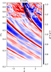 |
Fig. 1 HDBae simulation. 2D distribution in the (r, φ) plane of the mid-plane density, ρ, normalised over the azimuthally averaged value < ρ > at t = 10 orbits when the planet has just reached a Jovian mass. For the purposes of comparison with Fig. 6 of Bae et al. (2016), the y axis is plotted using a logarithmic scale. |
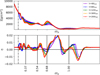 |
Fig. 2 Top panel: azimuthally averaged surface density profile for simulation HDBae. Bottom panel: azimuthally averaged η parameter. The planet is kept on a fixed circular orbit at r/rp = 1 and the ticks on the x axis (as well as the vertical black lines) indicate the values of η ~ 0 with a positive slope. The horizontal black line corresponds to η = 0. The damping region extends radially from rmin/r0 to the dot dashed line. |
4 Hydrodynamical case with complete treatment of radiative transport
The aim of this section is to study the propagation of density waves with a self-consistent treatment of radiation transport within the FLD approximation. With respect to the study presented in Bae et al. (2016) (and revisited in Section 3) we also considered a non-zero viscosity. In fact, discs have a low (but non-zero) bulk viscosity, as evidenced by observations (Pinte et al. 2016; Villenave et al. 2022) and supported by mechanisms such as the vertical shear instability (Nelson et al. 2013) leading to low viscosity in dead zones of the discs (where viscosity is not sustained by magnetorotational instability). The value of the alpha parameter αν is expected to be lower than 10−3 and possibly take values of the order of 10−4. In the following, we consider αν = 10−4.
Before inserting the planet, we ran a 2D axisymmetric (r, θ) simulation until the disc reaches thermal equilibrium. We notice that the main source of heating in a low-viscosity disc is the stellar heating. To recover the temperature profile of a stellar irradiated disc, we ran a 2D (r, θ) simulation, including the heating from a Solar-type star and using the temperature values of the resulting equilibrium disc as boundary for our 3D disc at the disc’s surface (as described in Lega et al. 2024). The equilibrium disc is flared (with flaring index 2/7) and has an aspect ratio of 0.03 at rp. The density slope, αΣ, (see Table 1) was chosen on the basis of a disc with constant star accretion rate (Lega et al. 2015). The mass flow carried by the disc was set to be ![Mathematical equation: $\[\dot{M} \sim 10^{-9} M_{\odot} / \mathrm{yr}\]$](/articles/aa/full_html/2025/10/aa55284-25/aa55284-25-eq31.png) , which is about one order of magnitude smaller than the typical accretion rate observed in young stars (Hartmann et al. 1998; Manara et al. 2016). We recovered typical star accretion rates by including non-ideal MHD effects (described in Section 5).
, which is about one order of magnitude smaller than the typical accretion rate observed in young stars (Hartmann et al. 1998; Manara et al. 2016). We recovered typical star accretion rates by including non-ideal MHD effects (described in Section 5).
Figure 4 shows the values of the equilibrium disc cooling time, density, and opacity in the (R, Z) plane. When looking at values of βc in Fig. 4 (left panel), the disc can be divided in two main regions based on the iso-contour line, logβc = 1. Specifically, inside the contour of logβc = 1 (Fig. 4, left panel), the cooling time values correspond to the regime of density wave propagation referred to as ‘adiabatic’ in Miranda & Rafikov (2020a) (see their Fig. 4). When inserting a planet in this region, we expect to find a gap at the planetary orbit and multiple rings and gaps in the inner region. Near the logβc = 1 contour, density waves are expected to be radiatively damped (see Ziampras et al. 2023). Finally, for logβc ≪ 1, the disc is in the locally isothermal regime. This regime is found near the disc surface, far from the planet’s forming region. We remark that the βc values are expected to change with time according to the perturbation introduced by the planet; thus, wave propagation regimes can be modified accordingly.
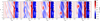 |
Fig. 3 Perturbed surface density of the HDBae simulation at the same snapshots represented in Fig. 2. The dashed lines indicate the radial position of the pressure bumps, i.e. the values of r for which η = 0 in Fig. 2. The dot-dashed line indicates the boundary of the damping region. |
 |
Fig. 4 Disc cooling time, density, and opacity in the (R, Z) ≡ (r sin(θ), r cos(θ)) plane of the disc in thermal equilibrium before the insertion of the planet. |
4.1 Jupiter-mass planet
Starting from the (R, Z) disc in thermal equilibrium, we expanded it in azimuth over the interval [−π, π] and restarted our simulation with an embedded planet. We ran the HDradJ simulation over 150 orbits at the planet location and obtained the azimuthally averaged values of βc, as well as the volume density and the optical thickness at the end of the integration (see Fig. 5). At the point, the planet has carved a gap and deeply modified the disc structure. However, the values of βc inside the planetary orbits are still compatible with the ‘adiabatic’ regime of wave propagation; thus, we would expect to find multiple gap and rings in the inner disc region (r < 4 au).
In Fig. 6, we show the perturbed surface density of the HDradJ simulation at different snapshots indicated in orbital period at the planet location: in the left panel, at t = 20 orbits, we clearly see the gap at the planet’s orbit and a primary ring of gas at the inner and outer gap edges (with the density maxima, respectively, at r ~ 4 and ~ 6.7 au) as well as the primary spiral arm. The secondary and a tertiary arms are clearly present inside the planetary orbit launched, respectively, at (r, φ) ~ (3.8, −π) and (r, φ) ~ (3.8, −1.8), propagating in the inner disc. The presence of multiple spiral arms is a necessary condition to have multiple gaps (Miranda & Rafikov 2019, 2020b). As for the primary gap at the planet’s orbit, multiple gaps form when density waves steepen into shocks depositing angular momentum into the gas. A second and a third ring at r ~ 3.3 and 2 au, respectively, are clearly formed at t = 100 (Fig. 6, second panel, and Fig. 7, top panel). Over the total integration time of 150 orbits, the primary gap is still evolving and rings of density maxima slightly move inwards and outwards as indicated by the vertical dotted lines in Fig. 6. The density contrast of the innermost ring increases with time while the second ring at r ~ 3.3 partially merges with the primary inner ring as the former eventually moves inwards.
From the computation of η (Fig. 7, bottom panel), we can see there is a pressure bump at the innermost ring at about 2 au, so that a reservoir of dust would be assumed to be trapped there, while the primary and secondary rings are marginally separated at t = 150 orbits. The pressure bump at about 3.3 au should stop dust from drifting inwards, thereby making a distinct reservoir with respect to the one centered at 2 au. The 3D fully radiative simulations require about a longer computational time by a factor of 10 with respect to isothermal or adiabatic simulations with controlled cooling2. The important result here is that distinct dust reservoirs can be formed in a realistic scenario, where thermal processes are computed in a self-consistent way.
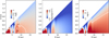 |
Fig. 5 Same as Fig. 4 for azimuthally averaged quantities for the 3D simulation HDradJ with an embedded Jupiter-mass planet. The snapshot corresponds to the end of the integration at 150 orbital periods at the planet location (5.2 au). |
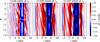 |
Fig. 6 Perturbed surface density of the HDradJ simulation at different snapshot indicated in orbital period at the planet location. The letters in the left and central panels indicate the primary (P), secondary (S), and tertiary (T) spiral arms. The dashed lines indicate the position the radial position of the pressure bumps, i.e. the values of r for which η = 0, with a positive slope, shown in Fig. 7. |
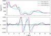 |
Fig. 7 Top panel: azimuthally averaged surface density profile for simulation HDradJ at the same snapshot represented in Fig. 6. Bottom panel: azimuthally averaged η values. The dashed line indicates the boundary of the damping region. |
4.2 Comparison with various EoSs
In this subsection, we consider simulations with an embedded Jupiter-mass planet (as in the HDradJ case, but using a different EoS) to compare the results obtained in HDradJ with different wave-damping regimes (see Miranda & Rafikov 2020a; Ziampras et al. 2023). In the following, we consider discs with respectively an isothermal EoS (HDiso), an adiabatic EoS with temperature relaxation to the initial value as in Eq. (1) (HDβc with βc = 1 and βc = 100) and an adiabatic case without thermal relaxation (HDadia).
We integrated the new simulations on longer timescales with respect to HDradJ taking advantage of shorter running times3 to check the persistence of rings and gap structures. Moreover, the disc domain is extended further in to investigate the possible formation of rings inside the one at 2 au obtained in the case of HDradJ; in addition, we sought to confirm that this inner-most ring at 2 au is not affected by the close inner disc boundary (which is at 1.5 au in HDradJ).
We show in Fig. 8 the perturbed surface density at t = 150 orbits at the planet location (top panels) and at t = 500 orbits (bottom panels) for all these cases; for comparison, we also inserted the results obtained before for the HDradJ case at t = 150 orbits between the two HDβc cases. As for the 2D case (Ziampras et al. 2020), the locally isothermal disc is the most efficient in forming multiple rings and gaps: three in our disc, which are also very contrasted (see Fig. 9, top panel), and are effective dust barriers based on the radial profile of η (Fig. 9, bottom panel). We confirm that we observed spiral arms extending further in, but no additional ring was observed inside r = 2 au.
At t = 500 orbits, the rings appear more contrasted with respect to t = 150 orbits, which is a good indication for their persistence. In all the cases, an innermost ring is formed close to r = 2 au, except in the case with βc = 1. According to the results obtained for 2D discs, this is the case where wave damping appears to be the most efficient (when no radiative effects are taken into account; see Ziampras et al. 2023).
We note the similarity between the fully radiative case and simulation HDβc with βc = 100 (i.e with a cooling time consistent with typical cooling times inside the Jupiter orbit; as shown in Fig. 5). We can also state that the ring at r = 2 au is not affected by the close radial boundary, since a very similar structure has been obtained in discs extending further in.
5 MHD simulation with prescribed cooling
In the previous section, we describe how the opening of secondary gaps by a Jupiter-mass planet is observed in low-viscosity 3D discs with a self-consistent treatment of the diffusion of heat. We consider the formation history of Jupiter by analyzing smaller masses in Section 6. In this section, we describe how low-viscosity discs transport gas towards the star at very low rates with respect to typical accretion rates observed in young stars (Hartmann et al. 1998; Manara et al. 2016). Instead, in magnetised discs embedded in warm fully ionised corona, gas transport at disc surface layers (at about two to three disc scale heights) can provide the required accretion flow onto the star, which we did not include in our simulation HDradJ. In fact, gas can flow inwards because of angular momentum removal by disc winds (Béthune et al. 2017; Lesur 2021b).
In the simulations presented here, we did not solve the radiation field; instead, we prescribed a warm corona via a steep vertical increase of the disc midplane temperature from three to five pressure scale heights. Precisely, similarly to Béthune et al. (2017), the disc is initialised with a temperature ratio between the corona and the disc Tcd = 6, as follows,
![Mathematical equation: $\[T(\tilde{\theta})=1+\left(T_{c d}-1\right)\left(\frac{1}{1+\exp [-6(|\tilde{\theta}|-4 h) / h]}\right)^2,\]$](/articles/aa/full_html/2025/10/aa55284-25/aa55284-25-eq32.png) (13)
(13)
where ![Mathematical equation: $\[\tilde{\theta} \equiv \pi / 2-\theta\]$](/articles/aa/full_html/2025/10/aa55284-25/aa55284-25-eq33.png) is the latitude, h is the disc aspect ratio (constant as our MHD discs are considered non-flared; see Appendix A). To this aim, we assumed the following function for the sound speed,
is the latitude, h is the disc aspect ratio (constant as our MHD discs are considered non-flared; see Appendix A). To this aim, we assumed the following function for the sound speed,
![Mathematical equation: $\[c_s(r, \theta)=\sqrt{\frac{G M_*}{r} h^2 T(\tilde{\theta})}.\]$](/articles/aa/full_html/2025/10/aa55284-25/aa55284-25-eq34.png) (14)
(14)
Considering the equations for vertical and rotational equilibrium, we provide in Appendix A the initial volume density and the initial azimuthal velocity we used in our MHD simulations. After the disc initialisation, we increased Tcd to 10 in the time interval [0 : 30] (code units).
The initial magnetic field is vertical B = Bz. Although there is a high level of uncertainty about the topology of the magnetic field of protoplanetary discs, their intensity is known to be weak (Lesur 2021b,a) in the sense that the midplane ratio of thermal over magnetic pressure: ![Mathematical equation: $\[\beta \equiv 2 \mu_{0} P / B_{z}^{2} \gg 1\]$](/articles/aa/full_html/2025/10/aa55284-25/aa55284-25-eq35.png) . Therefore, we considered discs with initial midplane values of β = 106, 105, 5 × 10³ and computed the radial profile of the magnetic field at midplane from β and from the midplane pressure, P = ρ(r, 0)cs(0)2.
. Therefore, we considered discs with initial midplane values of β = 106, 105, 5 × 10³ and computed the radial profile of the magnetic field at midplane from β and from the midplane pressure, P = ρ(r, 0)cs(0)2.
We did not solve the energy equation with the FLD approach (Eq. (2)) as in simulation HDradJ since this would require extremely long integration times for 3D MHD simulations. However, as we show in Fig. 8, when relaxing the internal energy to the initial temperature profile according to Eq. (1) on a cooling time βc = 100, we obtain results that are very similar to the fully radiative case. Therefore, we considered Eq. (1) in our MHD simulations with cooling time: βc = 100.
Before inserting the planet, we ran 2D (r, z) simulations for a few hundreds orbits at r = 1 au. At t = 300T0 (T0 = 2π yr) we show (Fig. 10, top panel) the density distribution on the (r, Z) plane for the case β = 5 × 10³ and ΛA = 1 (fiducial simulation). In Fig. 10 (top panel) we see that in the regime of Ohmic diffusion dominating over the Ambipolar one, there is no evidence of spontaneous generation. In other words, in the absence of the planet, the density distribution does not show rings and gaps (see e.g. Béthune et al. 2017). Therefore, when inserting a planet, any gap and ring formation will be a consequence of the perturbation induced by the planet itself. We also computed the mass flux as a function of r as
![Mathematical equation: $\[\dot{M}=2\left(\dot{M}_d+\dot{M}_w\right),\]$](/articles/aa/full_html/2025/10/aa55284-25/aa55284-25-eq37.png) (15)
(15)
where the factor of 2 takes into account the full disc. The quantities ![Mathematical equation: $\[\dot{M}_{d}\]$](/articles/aa/full_html/2025/10/aa55284-25/aa55284-25-eq38.png) and
and ![Mathematical equation: $\[\dot{M}_{w}\]$](/articles/aa/full_html/2025/10/aa55284-25/aa55284-25-eq39.png) are the mass flux of the disc region up to 2H and the corona from 2H to the disc surface, respectively. These quantities are computed from
are the mass flux of the disc region up to 2H and the corona from 2H to the disc surface, respectively. These quantities are computed from
![Mathematical equation: $\[\dot{M}_d=\int_0^{2 \pi} \int_{\theta_{2 H}}^{\pi / 2} \rho v_r r^2 ~sin (\theta) \mathrm{d} \theta \mathrm{d} \varphi.\]$](/articles/aa/full_html/2025/10/aa55284-25/aa55284-25-eq40.png) (16)
(16)
Here, θ2H is the colatitude at two disc scale heights and then we have
![Mathematical equation: $\[\dot{M}_w=\int_0^{2 \pi} \int_{\theta_0}^{\theta_{2 H}} \rho v_r r^2 ~sin (\theta) \mathrm{d} \theta \mathrm{d} \varphi,\]$](/articles/aa/full_html/2025/10/aa55284-25/aa55284-25-eq41.png) (17)
(17)
with θ(0) the value of the colatitude at the disc surface. In the bottom panel of Fig. 10, we plot this quantity averaged in time from 100 to 300T0 for our fiducial simulation. Negative values correspond to flux directed towards the star, while positive ones correspond to gas outflow. The corona appears to be dominated by disc out flowing wind while the disc accretes with values of ![Mathematical equation: $\[\dot{M} \sim 10^{-7} M_{\odot} / \mathrm{y}\]$](/articles/aa/full_html/2025/10/aa55284-25/aa55284-25-eq42.png) , similar to typical accretion rate observed in young stars (Hartmann et al. 1998; Manara et al. 2016). We provide in Appendix B an analysis of the mass flux from angular momentum conservation arguments.
, similar to typical accretion rate observed in young stars (Hartmann et al. 1998; Manara et al. 2016). We provide in Appendix B an analysis of the mass flux from angular momentum conservation arguments.
We let the planet growing for t = 10 orbital periods at the planet location and continued our simulation over 100 orbits. In Fig. 11, we show the perturbed surface density of our MHD runs at t = 100 orbits at rp = 5.2 au.
From left to right, we show the increased strength of the magnetic field and for a given value of the magnetic field, we can also increase the ambipolar diffusivity depending on the results obtained for multiple ring formation. For the lowest value of the magnetic field (β = 106, left panel), we see the formation of a secondary ring t about r = 2 au. In this case, we considered ΛA = 10, which corresponds to a very low effect of the non-ideal ambipolar diffusion effect. Keeping this same value of ΛA, and increasing the strength of the magnetic field (β = 105, second panel), we can scarcely identify the formation of a secondary ring. Instead, by increasing the ambipolar coefficient (ΛA = 1, third panel), we observe a significant enhancement of the secondary ring. By further increasing the magnetic field (β = 5 × 10³, right panels), we observe that the inner planet-induced spiral arms can be damped; in this case, no secondary ring would ever form at ΛA = 10 (not shown) or ΛA = 1 (fourth panel), while a weakly contrasted secondary ring appears for ΛA = 0.1 (fifth panel). Finally, a well-contrasted secondary ring appears in the right-most panel of Fig. 11 for ΛA = 0.01.
For the largest value of β, the magnetic field is immaterial and the formation of secondary rings closely resembles that occurring in purely hydrodynamical discs, regardless of the Ohmic and ambipolar diffusion coefficients. As the magnetic field increases (for smaller values of β), MHD effects come into play and the magnitude of ambipolar diffusion is found to have a strong impact on the existence of secondary rings.
This effect is similar to the one observed in the formation of zonal flow (Béthune et al. 2017; Riols et al. 2020) in disc regions where Ambipolar diffusion is the dominant non-ideal effect. In particular, spontaneous accumulations of gas are observed with anti-correlated concentrations of the vertical component of the magnetic field Bz. It has been shown (Béthune et al. 2017) that ambipolar diffusion is responsible for the accumulation of Bz. Therefore, if one or multiple gaps forms in a non-spontaneous way (e.g. because a massive planet perturbs the gas), then Bz will accumulate in the gaps (Wafflard-Fernandez & Lesur 2023) and lead to gas accumulation in rings, provided that the ambipolar diffusion is strong enough.
In Fig. 12, we show the azimuthally averaged surface density (top panel) and the η values (bottom panel) as a function of r at the same snapshot of Fig. 11. The plots correspond to the simulations presented in Fig. 11 for which a clearly contrasted secondary ring is formed (i.e. for β = 106 with ΛA = 10, for β = 105 with ΛA = 1, and for β = 5 × 10³ with ΛA = 0.01).
The values of η for both the primary and secondary rings at r 2 au reach values close to zero, although we do not observe a clear transition from negative to positive η, which is necessary for dust-trapping. A longer integration time would be required to verify whether dust-trapping is possible in these rings. Nevertheless, we consider very interesting that rings form for values of non-ideal parameters that are plausible in the disc region inside the Jupiter orbit.
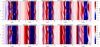 |
Fig. 8 Perturbed surface density at t = 150 orbits at the planet location (top panels) and at t = 500 (bottom panels) orbits. From left to right: simulation sets HDiso, HDβc with βc = 1, HDrad, and HDβc with βc = 100, HDadia. We observe multiple rings formation that depend on the EoS. Rings are persistent on longer integration times. For the radiative case, we report the last snapshot, i.e. the one at 150 orbits in the bottom panel. |
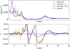 |
Fig. 9 Azimuthally averaged surface density profile (top) and the η values (bottom) for simulation sets HDiso, HDβc, and HDadia at t = 500 orbits at the planet’s location. |
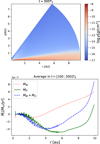 |
Fig. 10 Top panel: density distribution in the (r, Z) plane obtained for our simulation MHDβ5e3 with ΛA 1 at t = 300T0. Bottom panel: computation of |
![Mathematical equation: $\[\dot{M}(r, \theta)\]$](/articles/aa/full_html/2025/10/aa55284-25/aa55284-25-eq36.png)
 |
Fig. 11 Perturbed surface density of the MHD simulations. From left to right: increase in the strength of the magnetic field. In addition, for a given value of the magnetic field, we can also increase the Ambipolar coefficient value. For the lowest value of the magnetic field (left panel), we see the formation of a secondary ring at r = 2 au with our lower value of ambipolar diffusion (ΛA = 10); thus, we do not run additional simulations in this case. In the case of βm = 105 (second panel and third panels) we observe a secondary ring for ΛA = 10; however, the formation of a secondary well contrasted ring requires a higher ambipolar diffusion strength (ΛA = 1, third panel). Finally, for βm = 5 × 10³, there is no secondary ring formed for ΛA = 10 (not shown) nor for ΛA = 1 (fourth panel). We observe a poorly contrasted secondary ring for ΛA = 0.1 (fifth panel). Finally, we observe a well contrasted secondary ring for ΛA = 0.01 (right-most panel). |
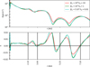 |
Fig. 12 Azimuthally averaged surface density profile (top) and azimuthally averaged η values (bottom) for MHD simulations presented in Fig. 11. Here, a well-contrasted secondary ring is formed. The planet is kept on a fixed circular orbit at rp = 5.2 au and the ticks on the x axis (as well as the vertical black lines) indicate the values of η ~ 0 with positive slope. The horizontal black line corresponds to η = 0. The damping region extends radially from rmin to the dotted line. |
6 Minimum planet mass for forming dust-trapping rings
It is well known (Lambrechts et al. 2014; Bitsch et al. 2018) that when a giant planet core reaches few tens of Earth masses, the so-called pebble isolation mass is reached and dust (at suited Stokes numbers) is blocked at the outer gap’s edge opened by the core. Moreover, in low-viscosity discs even cores of less than 20 Earth masses can open small gaps lowering the limit of the pebble isolation mass (see Bitsch et al. 2018). On the other hand, the dust inside the planet’s orbit drift towards the star and is eventually stopped at the inner (close to 1 au) pressure bump due do gas removal by magnetised winds (Suzuki et al. 2010; Ogihara et al. 2018).
We show in this paper that a Jupiter-mass planet has the ability to form multiple rings, according to disc thermal properties and to non-ideal magnetic diffusivities. However, such rings can be effective dust’s reservoirs if they form early on in the Jupiter formation history, possibly when Jupiter core has reached or slightly overcome the pebble isolation mass. Therefore, in this section, we describe the simulations we performed for a planet of a Saturn mass (simulation HDradS) and for a super-Earth of 30 Earth masses (simulation HDrad30) to check their ability to form multiple rings.
The super-Earth opens a gap and forms a secondary ring (at ~3.8 au). which increases in density contrast on long integration times (see Fig. 13). A third density maximum appears which, however, is not associated to a local pressure maximum since it has η > 0. Instead, three rings appear for Saturn at 150 orbits and two for Jupiter, as previously discussed. The values of r for which η = 0 move inwards when we are increasing the planet’s mass.
From Fig. 13, we can propose the following evolutionary picture. When a planet reaches the pebble isolation mass, it starts trapping dust at two locations near the inner edge of its gap. As the planet grows in mass, the locations of these two rings shift inwards, together with their dust. Near the mass of Saturn, a third ring appears near 3 au, trapping the dust that had not been trapped in the two other rings (unless the planet grows so slowly that all the untrapped dust has already drifted into the star). As the planet grows further, the two initial rings merge and the last one moves from ~3 to ~2 au. Obviously, this picture does not take into account that the planet is migrating at the same time. However, in the case of a proto-Jupiter, its migration may have been stalled or even reversed by the appearance of a proto-Saturn (Walsh et al. 2011).
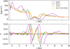 |
Fig. 13 Top panel: azimuthally averaged surface density profile for simulations Hrad30, HradS and HradJ at 150 orbital periods at the planet location. Bottom panel: azimuthally averaged η values. Colour markers at η = 0 with a positive slope identify the position of the pressure bumps on the top panel. |
7 Conclusion
Cosmochemical observations provide evidence that millimetresize dust remained trapped in the inner part of the disc for a timescale of at least a million years. Multiple trapping sites would have had to exist to explain the formation of four families of chondrites, which are chemically and isotopically distinct from each other.
In this work, we have explored the possibility that Jupiter formed local maxima in the azimuthally averaged pressure in the inner part of the protoplanetary disc (inwards of its orbit). These averaged pressure bumps are potential sites of dust-trapping, but the actual response of dust to the non-axisymmetric features that characterise these bumps remains to be investigated.
We have shown that in a low-viscosity disc, the opening of secondary gaps and density bumps is robust. This was also observed in our 3D simulations when we self-consistently simulated the diffusion of heat, giving a cooling timescale of about 100 orbital times in the inner disc.
When considering a strong magnetic field, we observe that the inner planet-induced spiral arm can be damped and a secondary ring forms only if ambipolar diffusion is strong enough. Further work is warranted to assess the origin of this damping. We note that it could arise from dissipation, when the diffusion coefficients are at adequate levels, or from a removal of the angular momentum flux by the wind. We remark that self-consistent disc ionisation models show that the appropriate parameters for non-ideal MHD are consistent with those for which we observed the effective formation of secondary gaps and rings in our simulations.
A planet seems to be able to open secondary gaps and trap dust in rings when it reaches a mass close to the pebble isolation mass. Thus, as it cuts the flow of dust from the outer disc across its orbit, it also traps part of the dust in rings located inwards of its orbit. As the planet grows, these rings move away from the planet and can merge with each other, while a new ring can be formed farther away. Coupled with planet migration, these results provide a new view of the non-trivial evolution of dust in the inner Solar System, which may be consistent with cosmochemical constraints on dust preservation and confinement on extended timescales.
Acknowledgements
A.M. is grateful for support from the ERC advanced grant HolyEarth N. 101019380. This work was granted access to the HPC resources of IDRIS and CINES under the allocation A0160407233 made by GENCI. F.M. acknowledges support from UNAM’s grant PAPIIT 107723, UNAM’s DGAPA PASPA program and the Laboratoire Lagrange at Observatoire de la Côte d’Azur for hospitality during a one-year sabbatical stay. E.L. wish to thank Alain Miniussi for maintenance and re-factorisation of the code fargOCA. This work was supported by the French government through the France 2030 investment plan managed by the National Research Agency (ANR), as part of the Initiative of Excellence Université Côte d’Azur under reference number ANR-15-IDEX-01.
Appendix A Setting initial conditions for MHD simulations
We describe the method we used to determine the initial conditions for our MHD simulations described in Section 5 in order to model discs with a warm corona. To this aim we start with a corona mildly hotter than the disc’s midplane, and determine the vertical density and rotational velocity profiles that correspond to strict hydrostatic and centrifugal equilibria. We then progressively increase the corona’s temperature until we reach the desired corona to disc temperature ratio.
We assume that the sound speed is inversely proportional to the spherical radius and has a separable dependence on r and θ:
![Mathematical equation: $\[c_s^2(r)=\left(c_{s 0}^0\right)^2\left(\frac{r}{r_0}\right)^{-1} g(\theta),\]$](/articles/aa/full_html/2025/10/aa55284-25/aa55284-25-eq43.png) (A.1)
(A.1)
where g(θ) is an even function with respect to π/2 and g(π/2) = 1 and r0 is an arbitrary reference radius where the sound speed, at the midplane, is ![Mathematical equation: $\[c_{s 0}^{0}\]$](/articles/aa/full_html/2025/10/aa55284-25/aa55284-25-eq44.png) . We have considered for g(θ) the function
. We have considered for g(θ) the function ![Mathematical equation: $\[T(\tilde{\theta})\]$](/articles/aa/full_html/2025/10/aa55284-25/aa55284-25-eq45.png) defined in Eq. 13. We consider a constant disc aspect ratio:
defined in Eq. 13. We consider a constant disc aspect ratio:
![Mathematical equation: $\[h(r)=\frac{c_{s 0}(r)}{v_K(r)}=\mathrm{const},\]$](/articles/aa/full_html/2025/10/aa55284-25/aa55284-25-eq46.png) (A.2)
(A.2)
where ![Mathematical equation: $\[v_{K}(r)=\sqrt{\frac{G M_{*}}{r}}\]$](/articles/aa/full_html/2025/10/aa55284-25/aa55284-25-eq47.png) is the circular Keplerian velocity at mid-plane, which implies that
is the circular Keplerian velocity at mid-plane, which implies that ![Mathematical equation: $\[c_{s 0}^{0} \equiv h v_{k}\left(r_{0}\right)\]$](/articles/aa/full_html/2025/10/aa55284-25/aa55284-25-eq48.png) .
.
The equations for rotational and vertical equilibrium in spherical coordinates are
![Mathematical equation: $\[-\frac{\partial_r\left(\rho_0 c_s^2\right)}{\rho_0}+\frac{v_\phi^2}{r}-\frac{G M_*}{r^2}=0,\]$](/articles/aa/full_html/2025/10/aa55284-25/aa55284-25-eq49.png) (A.3)
(A.3)
![Mathematical equation: $\[-\frac{1}{r} \frac{\partial_\theta\left(\rho_0 c_s^2\right)}{\rho_0}+\frac{v_\phi^2}{r} \cot \theta=0.\]$](/articles/aa/full_html/2025/10/aa55284-25/aa55284-25-eq50.png) (A.4)
(A.4)
Here, we have ρ0 and ![Mathematical equation: $\[c_{s 0}(r)=c_{s 0}^{0} \times\left(\frac{r_{0}}{r}\right)^{1 / 2}\]$](/articles/aa/full_html/2025/10/aa55284-25/aa55284-25-eq51.png) respectively the density and the sound speed at the midplane at radius r. We introduce notations similar to those of Masset & Benítez-Llambay (2016) and define
respectively the density and the sound speed at the midplane at radius r. We introduce notations similar to those of Masset & Benítez-Llambay (2016) and define
![Mathematical equation: $\[L=\log \rho_0, \quad v=\log \left(\frac{r}{r_0}\right), \quad u=-\log (\sin~ \theta).\]$](/articles/aa/full_html/2025/10/aa55284-25/aa55284-25-eq52.png)
Equations (A.3) and (A.4) become
![Mathematical equation: $\[-c_s^2 \partial_v L+c_s^2+v_\phi^2-\frac{G M_*}{r}=0,\]$](/articles/aa/full_html/2025/10/aa55284-25/aa55284-25-eq53.png) (A.5)
(A.5)
![Mathematical equation: $\[c_{s 0}^2(r) \frac{\partial_u\left[\rho_0 g(\theta)\right]}{\rho_0}+v_\phi^2=0.\]$](/articles/aa/full_html/2025/10/aa55284-25/aa55284-25-eq54.png) (A.6)
(A.6)
Introducing ![Mathematical equation: $\[m \equiv \frac{v_{\phi}^{2}}{c_{s}^{2}}\]$](/articles/aa/full_html/2025/10/aa55284-25/aa55284-25-eq55.png) , we get:
, we get:
![Mathematical equation: $\[-\partial_v L+1+m-\frac{G M_*}{r c_s^2}=0,\]$](/articles/aa/full_html/2025/10/aa55284-25/aa55284-25-eq56.png) (A.7)
(A.7)
![Mathematical equation: $\[c_{s 0}^2 g(u) \partial_u L+c_{s 0}^2 \partial_u g(u)+v_\phi^2=0.\]$](/articles/aa/full_html/2025/10/aa55284-25/aa55284-25-eq57.png) (A.8)
(A.8)
As per our assumption of a constant aspect ratio, ![Mathematical equation: $\[K \equiv \frac{G M_{*}}{r c_{s 0}^{2}}\]$](/articles/aa/full_html/2025/10/aa55284-25/aa55284-25-eq58.png) is a constant and the equations above can be recast as:
is a constant and the equations above can be recast as:
![Mathematical equation: $\[-\partial_v L+1+m-\frac{K}{g(u)}=0,\]$](/articles/aa/full_html/2025/10/aa55284-25/aa55284-25-eq59.png) (A.9)
(A.9)
![Mathematical equation: $\[\partial_u L+\frac{\partial_u g(u)}{g(u)}+m=0.\]$](/articles/aa/full_html/2025/10/aa55284-25/aa55284-25-eq60.png) (A.10)
(A.10)
Define ![Mathematical equation: $\[G(u)=\frac{1}{g(u)}\]$](/articles/aa/full_html/2025/10/aa55284-25/aa55284-25-eq61.png) , and L′ = L + log g(u), giving:
, and L′ = L + log g(u), giving:
![Mathematical equation: $\[-\partial_v L^{\prime}+1+m-K G(u)=0,\]$](/articles/aa/full_html/2025/10/aa55284-25/aa55284-25-eq62.png) (A.11)
(A.11)
![Mathematical equation: $\[\partial_u L^{\prime}+m=0.\]$](/articles/aa/full_html/2025/10/aa55284-25/aa55284-25-eq63.png) (A.12)
(A.12)
Let m′ = m − KG(u), thus, we have
![Mathematical equation: $\[-\partial_v L^{\prime}+1+m^{\prime}=0,\]$](/articles/aa/full_html/2025/10/aa55284-25/aa55284-25-eq64.png) (A.13)
(A.13)
![Mathematical equation: $\[\partial_u L^{\prime}+m^{\prime}+K G(u)=0.\]$](/articles/aa/full_html/2025/10/aa55284-25/aa55284-25-eq65.png) (A.14)
(A.14)
The values of m′ and L′ are determined using a method of characteristics. We introduce the following combinations of the coordinates u and v:
![Mathematical equation: $\[s=u+v,\]$](/articles/aa/full_html/2025/10/aa55284-25/aa55284-25-eq66.png) (A.15)
(A.15)
![Mathematical equation: $\[s^{\prime}=u-v,\]$](/articles/aa/full_html/2025/10/aa55284-25/aa55284-25-eq67.png) (A.16)
(A.16)
so
![Mathematical equation: $\[u=\frac{1}{2}\left(s+s^{\prime}\right),\]$](/articles/aa/full_html/2025/10/aa55284-25/aa55284-25-eq68.png) (A.17)
(A.17)
![Mathematical equation: $\[v=\frac{1}{2}\left(s-s^{\prime}\right).\]$](/articles/aa/full_html/2025/10/aa55284-25/aa55284-25-eq69.png) (A.18)
(A.18)
Using Eqs. A.13 and A.14, we derive
![Mathematical equation: $\[\partial_s m^{\prime}=\frac{1}{2}\left(\partial_u m^{\prime}+\partial_v m^{\prime}\right)=0\]$](/articles/aa/full_html/2025/10/aa55284-25/aa55284-25-eq70.png)
Thus, m′ depends only on s′, and its dependence on s′ can be determined at the midplane. Considering a constant h and a midplane density, ![Mathematical equation: $\[\rho_{mid}=\frac{\Sigma_{0}\left(r / r_{0}\right)^{-\alpha_{\Sigma}-1}}{\sqrt{2 \pi} h}\]$](/articles/aa/full_html/2025/10/aa55284-25/aa55284-25-eq71.png) , we obtain from Eq. A.13:
, we obtain from Eq. A.13:
![Mathematical equation: $\[\xi+1+m^{\prime}=0 \Rightarrow m^{\prime}=-\xi-1,\]$](/articles/aa/full_html/2025/10/aa55284-25/aa55284-25-eq72.png)
with ξ = αΣ + 1 Hence,
![Mathematical equation: $\[m=h^{-2} G(u)-1-\xi.\]$](/articles/aa/full_html/2025/10/aa55284-25/aa55284-25-eq73.png) (A.19)
(A.19)
From Eq. (A.14), we get
![Mathematical equation: $\[\partial_u L^{\prime}+h^{-2} G(u)-1-\xi=0.\]$](/articles/aa/full_html/2025/10/aa55284-25/aa55284-25-eq74.png) (A.20)
(A.20)
Letting ![Mathematical equation: $\[W(u)=\int_0^u G\left(u^{\prime}\right) d u^{\prime}\]$](/articles/aa/full_html/2025/10/aa55284-25/aa55284-25-eq75.png) , we have
, we have
![Mathematical equation: $\[L^{\prime}(u)=L^{\prime}(0)-h^{-2} W(u)+(1+\xi) u,\]$](/articles/aa/full_html/2025/10/aa55284-25/aa55284-25-eq76.png)
hence
![Mathematical equation: $\[L(u)=-\log g(u)+L(0)-h^{-2} W(u)+(1+\xi) u.\]$](/articles/aa/full_html/2025/10/aa55284-25/aa55284-25-eq77.png)
Thus, the density profile is
![Mathematical equation: $\[\rho(u)=\frac{1}{g(u)} \rho_{\text {mid }} \exp \left[-h^{-2} W(u)+(1+\xi) u\right],\]$](/articles/aa/full_html/2025/10/aa55284-25/aa55284-25-eq78.png) (A.21)
(A.21)
![Mathematical equation: $\[=\rho_{00}\left(\frac{r}{r_0}\right)^{-\xi}(\sin~ \theta)^{-1-\xi} G(u) \exp \left[-h^{-2} W(u)\right],\]$](/articles/aa/full_html/2025/10/aa55284-25/aa55284-25-eq79.png) (A.22)
(A.22)
with ![Mathematical equation: $\[\rho_{00}=\frac{\Sigma_{0}}{\sqrt{2 \pi} h}\]$](/articles/aa/full_html/2025/10/aa55284-25/aa55284-25-eq80.png) . Finally, from the expression for m (Eq. A.19), the azimuthal velocity is
. Finally, from the expression for m (Eq. A.19), the azimuthal velocity is
![Mathematical equation: $\[v_\phi^2=\left(c_{s 0}\right)^2 h^{-2}-(1+\xi) c_s^2 \text {, }\]$](/articles/aa/full_html/2025/10/aa55284-25/aa55284-25-eq81.png) (A.23)
(A.23)
![Mathematical equation: $\[=\left(c_{s 0}^0\right)^2\left(\frac{r_0}{r}\right) \frac{G M_*}{r_0\left(c_{s 0}^0\right)^2}-(1+\xi) c_s^2,\]$](/articles/aa/full_html/2025/10/aa55284-25/aa55284-25-eq82.png) (A.24)
(A.24)
![Mathematical equation: $\[=\frac{G M_*}{r}-(1+\xi) c_s^2.\]$](/articles/aa/full_html/2025/10/aa55284-25/aa55284-25-eq83.png) (A.25)
(A.25)
Appendix B MHD simulations diagnostics
In the following, we provide some diagnostics on our MHD simulations based on the study of mass transport through the disc in terms or mass flux or mass accretion (or mass loss through the wind) rates.
The radial mass flux is generated by torques that determine a loss of angular momentum. We follow Béthune et al. (2017) and compute quantities defined in their Eqs. 8 and 9 and reported here:
The azimuthal average of a quantity X is denoted as
![Mathematical equation: $\[<X>_{\varphi}=\frac{1}{\Delta \varphi} \int_0^{\Delta \varphi} X(r, \theta, \phi, t) d \phi\]$](/articles/aa/full_html/2025/10/aa55284-25/aa55284-25-eq84.png)
Radial profiles are obtained by vertical integration in the disc domain,
![Mathematical equation: $\[<X>_{\varphi, \theta}=\frac{1}{2 H(r)} \int_{-H(r)}^{H(r)}<X>_{\varphi}(r, \theta, t) d \theta\]$](/articles/aa/full_html/2025/10/aa55284-25/aa55284-25-eq85.png)
A density weighted quantity is denoted as
![Mathematical equation: $\[<X>_\rho=\frac{<\rho X>_{\varphi, \theta}}{<\rho>_{\varphi, \theta}}\]$](/articles/aa/full_html/2025/10/aa55284-25/aa55284-25-eq86.png)
-
The fluctuating Reynold stress tensor is defined by:
![Mathematical equation: $\[\mathcal{R} \equiv \rho \tilde{\mathbf{v}} \otimes \tilde{\mathbf{v}}\]$](/articles/aa/full_html/2025/10/aa55284-25/aa55284-25-eq87.png)
where
![Mathematical equation: $\[\tilde{\mathbf{v}}=\mathbf{v}-\lt v\gt_{\rho}\]$](/articles/aa/full_html/2025/10/aa55284-25/aa55284-25-eq88.png) .
. -
The Maxwell stress tensor is:
![Mathematical equation: $\[\mathcal{M} \equiv-\mathbf{B} \otimes \mathbf{B}\]$](/articles/aa/full_html/2025/10/aa55284-25/aa55284-25-eq89.png)
and we call 𝒯 ≡ ℛ + ℳ
-
We use the same notation as Shakura & Sunyaev (1973) to define α values by normalising with vertically integrated pressure:
![Mathematical equation: $\[\alpha^{\mathcal{R}}(r, \theta, t)=\frac{<\mathcal{R}>_{\varphi}}{<P>_{\varphi, \theta}}\]$](/articles/aa/full_html/2025/10/aa55284-25/aa55284-25-eq90.png) (B.1)
(B.1)and similarly for values associated to the magnetic field, denoted αℳ.
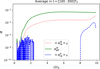 |
Fig. B.1 Computation of the α values from Eq.B.1 averaged over time for the fiducial MHD simulation with β = 5 103 and ΛA = 1. |
The radial mass flux can be deduced from the conservation of angular momentum, provided Σ(r) = 2H(r) < ρ >φ,θ:
![Mathematical equation: $\[\begin{cases}\Sigma(r)<v_r>_\rho & \equiv \tau_r+\tau_z \\ \tau_r & \simeq-\frac{1}{r\left(\partial_r<r v_{\varphi}>_{\varphi, \theta}\right)} \partial_r\left(2 r^2 H(r)<\mathcal{T}_{r, \varphi}>_{\varphi, \theta}\right) \\ \tau_z & \simeq-\frac{r}{\left[\partial_r<r v_{\varphi}>_{\varphi, \theta}\right]}\left(<\mathcal{T}_{\varphi, \theta}>_{\varphi}\right)_{-H}^{+H}\end{cases}\]$](/articles/aa/full_html/2025/10/aa55284-25/aa55284-25-eq91.png) (B.2)
(B.2)
where τr gives the mass flux due to the radial component of the angular momentum and τz gives the mass transport due to angular momentum extracted at disc surfaces z = ±H
In Figure B.1, we clearly see that the α values associated to the magnetic field dominate with respect to the Reynold α values. From Fig. B.2, we can appreciate that the 1.h.s. and the sum of the τ component of the r.h.s. of the equation follow nicely the same trend both when averaged on time and on space in the interval r ∈ [2 : 8]r0. Moreover, in this radial interval there is no contribution to the mass flux from the radial transport of the angular momentum. Precisely, let’s notice (Fig.B.1), that ![Mathematical equation: $\[\lt\alpha_{r \varphi}^{\mathcal{M}}\gt_{\varphi, \theta}\]$](/articles/aa/full_html/2025/10/aa55284-25/aa55284-25-eq92.png) is practically constant for r ∈ [2 : 8]r0, and it is the divergence of this term (i.e of 𝒯rφ in Eq.B.2) that contributes to the radial mass transport.
is practically constant for r ∈ [2 : 8]r0, and it is the divergence of this term (i.e of 𝒯rφ in Eq.B.2) that contributes to the radial mass transport.
Therefore, the mass flux is completely due to the angular momentum extracted from the disc in the vertical direction (in this case it is the value of 𝒯φ,θ in Eq.B.2 at z = ±H that contributes to τθ). This result is in agreement with the one described in the fiducial simulation of Béthune et al. (2017) (their Fig.7).
Appendix C Boundary conditions for MHD simulations
In our MHD simulations, we considered the following boundary conditions:
Hydrodynamical quantities:
Inner radial boundary: We extrapolated the density and the energy from the active cells into the ghost cells according to the initial power law profile. We extrapolated the azimuthal velocity component of the active cells into the ghost cells according to the Keplerian profile. The polar component of the velocity was copied from the active cell into the ghosts cells. We closed the inner boundary by setting to zero the radial component of the velocity.
Outer radial boundary: We extrapolated the density and the energy from the active cells into the ghost cells according to the initial power law profile. The azimuthal component of the velocity was extrapolated according to the Keplerian profile. The polar component of the velocity was copied from the active cell into the ghosts cells. For the radial velocity component, we compared the value of the active cell to a threshold value
![Mathematical equation: $\[\tilde{v}_{r}\]$](/articles/aa/full_html/2025/10/aa55284-25/aa55284-25-eq93.png) proportional to a fraction of the sound speed. We set the velocity in the ghost cells equal to
proportional to a fraction of the sound speed. We set the velocity in the ghost cells equal to ![Mathematical equation: $\[\tilde{v}_{r}\]$](/articles/aa/full_html/2025/10/aa55284-25/aa55284-25-eq94.png) if the velocity of the active cell is smaller than the threshold value; otherwise, we simply copied the value of the active cell into the ghosts.
if the velocity of the active cell is smaller than the threshold value; otherwise, we simply copied the value of the active cell into the ghosts.Polar boundaries We extrapolated the density and the energy fields according to the hydrostatic vertical equilibrium defined in Appendix A. We extrapolated the azimuthal velocity according to rotational equilibrium (Appendix A). We copied the radial and the vertical components of the velocity from the active cells into the ghost cells.
Magnetic field components and EMF
Inner and outer radial boundary: We linearly extrapolated the values of the electromotive forces from the active cells into the ghost cells. We copied the azimuthal and the vertical components of the magnetic field from the active cells into the ghosts. We derived the radial component of the magnetic field by requiring that the divergence of the magnetic field in the ghost cells is zero.
Polar boundaries We linearly extrapolated the values of the electromotive forces from the active cells into the ghost cells. We copied the azimuthal and the radial components of the magnetic field from the active cells into the ghosts. We derived the polar component of the magnetic field by requiring that the divergence of the magnetic field in the ghost cells is zero.
Finally, we imposed a density floor by requiring that the minimum value of the density is given by:
![Mathematical equation: $\[\rho_{min }=\frac{B_r^2+B_\theta^2+B_{\varphi}^2}{4 v_{k i n} \mu_0}\]$](/articles/aa/full_html/2025/10/aa55284-25/aa55284-25-eq95.png) (C.1)
(C.1)
where vkin is the Keplerian velocity at the inner radial boundary. In other words, we forced the Alfvén speed to remain lower than few times the Keplerian velocity at the inner boundary.
References
- Andrews, S. M., Huang, J., Pérez, L. M., et al. 2018, ApJ, 869, L41 [NASA ADS] [CrossRef] [Google Scholar]
- Armitage, P. J. 2011, Ann. Rev. Astron. Astrophys., 49, 195 [Google Scholar]
- Bae, J., Nelson, R. P., & Hartmann, L. 2016, ApJ, 833, 126 [NASA ADS] [CrossRef] [Google Scholar]
- Bae, J., Zhu, Z., & Hartmann, L. 2017, ApJ, 850, 201 [NASA ADS] [CrossRef] [Google Scholar]
- Bai, X.-N. 2017, ApJ, 845, 75 [NASA ADS] [CrossRef] [Google Scholar]
- Bell, K. R., & Lin, D. N. C. 1994, ApJ, 427, 987 [NASA ADS] [CrossRef] [Google Scholar]
- Benítez-Llambay, P., & Masset, F. S. 2016, ApJS, 223, 11 [Google Scholar]
- Béthune, W., Lesur, G., & Ferreira, J. 2017, A&A, 600, A75 [NASA ADS] [CrossRef] [EDP Sciences] [Google Scholar]
- Bitsch, B., Crida, A., Morbidelli, A., Kley, W., & Dobbs-Dixon, I. 2013, A&A, 549, A124 [NASA ADS] [CrossRef] [EDP Sciences] [Google Scholar]
- Bitsch, B., Morbidelli, A., Johansen, A., et al. 2018, A&A, 612, A30 [NASA ADS] [CrossRef] [EDP Sciences] [Google Scholar]
- Brasser, R., & Mojzsis, S. J. 2020, Nat. Astron., 4, 492 [NASA ADS] [CrossRef] [Google Scholar]
- Commerçon, B., Teyssier, R., Audit, E., Hennebelle, P., & Chabrier, G. 2011, A&A, 529, A35 [NASA ADS] [CrossRef] [EDP Sciences] [Google Scholar]
- Cui, C., & Bai, X.-N. 2021, MNRAS, 507, 1106 [NASA ADS] [CrossRef] [Google Scholar]
- de Val-Borro, M., Edgar, R. G., Artymowicz, P., et al. 2006, MNRAS, 370, 529 [Google Scholar]
- Fukuda, K., Tenner, T. J., Kimura, M., et al. 2022, Geochim. Cosmochim. Acta, 322, 194 [NASA ADS] [CrossRef] [Google Scholar]
- Gressel, O., Turner, N. J., Nelson, R. P., & McNally, C. P. 2015, ApJ, 801, 84 [NASA ADS] [CrossRef] [Google Scholar]
- Hartmann, L., Calvet, N., Gullbring, E., & D’Alessio, P. 1998, ApJ, 495, 385 [Google Scholar]
- Haugbølle, T., Weber, P., Wielandt, D. P., et al. 2019, AJ, 158, 55[0pt] [Google Scholar]
- Hopkins, P. F., Squire, J., Skalidis, R., & Soliman, N. H. 2024, arXiv e-prints [arXiv:2405.06026] [Google Scholar]
- Hubeny, I. 1990, ApJ, 351, 632 [NASA ADS] [CrossRef] [Google Scholar]
- Kleine, T., Budde, G., Burkhardt, C., et al. 2020, Space Sci. Rev., 216, 55 [CrossRef] [Google Scholar]
- Kley, W., Bitsch, B., & Klahr, H. 2009, A&A, 506, 971 [NASA ADS] [CrossRef] [EDP Sciences] [Google Scholar]
- Kruijer, T. S., Burkhardt, C., Budde, G., & Kleine, T. 2017, Proc. Natl. Acad. Sci., 114, 6712 [Google Scholar]
- Lambrechts, M., Johansen, A., & Morbidelli, A. 2014, A&A, 572, A35 [NASA ADS] [CrossRef] [EDP Sciences] [Google Scholar]
- Lega, E., Crida, A., Bitsch, B., & Morbidelli, A. 2014, MNRAS, 440, 683 [Google Scholar]
- Lega, E., Morbidelli, A., Bitsch, B., Crida, A., & Szulágyi, J. 2015, MNRAS, 452, 1717 [Google Scholar]
- Lega, E., Benisty, M., Cridland, A., et al. 2024, A&A, 690, A183 [NASA ADS] [CrossRef] [EDP Sciences] [Google Scholar]
- Lesur, G. 2021a, J. Plasma Phys., 87, 205870101 [CrossRef] [Google Scholar]
- Lesur, G. R. J. 2021b, A&A, 650, A35 [NASA ADS] [CrossRef] [EDP Sciences] [Google Scholar]
- Levermore, C. D., & Pomraning, G. C. 1981, ApJ, 248, 321 [NASA ADS] [CrossRef] [Google Scholar]
- Lyra, W., Richert, A. J. W., Boley, A., et al. 2016, ApJ, 817, 102 [NASA ADS] [CrossRef] [Google Scholar]
- Manara, C. F., Rosotti, G., Testi, L., et al. 2016, A&A, 591, L3 [NASA ADS] [CrossRef] [EDP Sciences] [Google Scholar]
- Masset, F. 2000, A&AS, 141, 165 [NASA ADS] [CrossRef] [EDP Sciences] [Google Scholar]
- Masset, F. S., & Benítez-Llambay, P. 2016, ApJ, 817, 19 [NASA ADS] [CrossRef] [Google Scholar]
- Menou, K., & Goodman, J. 2004, ApJ, 606, 520 [NASA ADS] [CrossRef] [Google Scholar]
- Mihalas, D., & Mihalas, B. W. 1984, Foundations of Radiation Hydrodynamics (USA: Courier Corporation) [Google Scholar]
- Miranda, R., & Rafikov, R. R. 2019, ApJ, 875, 37 [Google Scholar]
- Miranda, R., & Rafikov, R. R. 2020a, ApJ, 904, 121 [NASA ADS] [CrossRef] [Google Scholar]
- Miranda, R., & Rafikov, R. R. 2020b, ApJ, 892, 65 [NASA ADS] [CrossRef] [Google Scholar]
- Nakagawa, Y., Sekiya, M., & Hayashi, C. 1986, Icarus, 67, 375 [Google Scholar]
- Nanne, J. A. M., Nimmo, F., Cuzzi, J. N., & Kleine, T. 2019, Earth Planet. Sci. Lett., 511, 44 [CrossRef] [Google Scholar]
- Nelson, R. P., Gressel, O., & Umurhan, O. M. 2013, MNRAS, 435, 2610 [Google Scholar]
- Neumann, W., Breuer, D., & Spohn, T. 2012, A&A, 543, A141 [NASA ADS] [CrossRef] [EDP Sciences] [Google Scholar]
- Ogihara, M., Kokubo, E., Suzuki, T. K., & Morbidelli, A. 2018, A&A, 612, L5 [NASA ADS] [CrossRef] [EDP Sciences] [Google Scholar]
- Pinte, C., Dent, W. R. F., Ménard, F., et al. 2016, ApJ, 816, 25 [Google Scholar]
- Piralla, M., Villeneuve, J., Schnuriger, N., Bekaert, D. V., & Marrocchi, Y. 2023, Icarus, 394, 115427 [NASA ADS] [CrossRef] [Google Scholar]
- Riols, A., & Lesur, G. 2018, A&A, 617, A117 [NASA ADS] [CrossRef] [EDP Sciences] [Google Scholar]
- Riols, A., Lesur, G., & Menard, F. 2020, A&A, 639, A95 [NASA ADS] [CrossRef] [EDP Sciences] [Google Scholar]
- Schneider, J. M., Burkhardt, C., Marrocchi, Y., Brennecka, G. A., & Kleine, T. 2020, Earth Planet. Sci. Lett., 551, 116585 [CrossRef] [Google Scholar]
- Shakura, N. I., & Sunyaev, R. A. 1973, A&A, 24, 337 [NASA ADS] [Google Scholar]
- Stone, J. M., Mihalas, D., & Norman, M. L. 1992, ApJS, 80, 819 [CrossRef] [Google Scholar]
- Suzuki, T. K., Muto, T., & Inutsuka, S.-i. 2010, ApJ, 718, 1289 [NASA ADS] [CrossRef] [Google Scholar]
- Takeuchi, T., & Lin, D. N. C. 2002, ApJ, 581, 1344 [NASA ADS] [CrossRef] [Google Scholar]
- Villenave, M., Stapelfeldt, K. R., Duchêne, G., et al. 2022, ApJ, 930, 11 [NASA ADS] [CrossRef] [Google Scholar]
- Wafflard-Fernandez, G., & Lesur, G. 2023, A&A, 677, A70 [NASA ADS] [CrossRef] [EDP Sciences] [Google Scholar]
- Walsh, K. J., Morbidelli, A., Raymond, S. N., O’Brien, D. P., & Mandell, A. M. 2011, Nature, 475, 206 [Google Scholar]
- Warren, P. H. 2011, Earth Planet. Sci. Lett., 311, 93 [Google Scholar]
- Zhang, S., Zhu, Z., Huang, J., et al. 2018, ApJ, 869, L47 [Google Scholar]
- Ziampras, A., Kley, W., & Dullemond, C. P. 2020, A&A, 637, A50 [NASA ADS] [CrossRef] [EDP Sciences] [Google Scholar]
- Ziampras, A., Nelson, R. P., & Rafikov, R. R. 2023, MNRAS, 524, 3930 [NASA ADS] [CrossRef] [Google Scholar]
The integral form is preferred to avoid the computation of the divergence.
The diffusion part of the energy equation is solved implicitly and this often requires a large number of iterations for the numerical scheme to reach convergence.
About 2.5 hours for 10 orbits at the planet location on 1 GPU AMD MI250 to be compared with 2.5 hours for 1 orbit on 96 cores on AMD Genoa EPYC 9654.
All Tables
All Figures
|
Fig. 1 HDBae simulation. 2D distribution in the (r, φ) plane of the mid-plane density, ρ, normalised over the azimuthally averaged value < ρ > at t = 10 orbits when the planet has just reached a Jovian mass. For the purposes of comparison with Fig. 6 of Bae et al. (2016), the y axis is plotted using a logarithmic scale. |
| In the text | |
|
Fig. 2 Top panel: azimuthally averaged surface density profile for simulation HDBae. Bottom panel: azimuthally averaged η parameter. The planet is kept on a fixed circular orbit at r/rp = 1 and the ticks on the x axis (as well as the vertical black lines) indicate the values of η ~ 0 with a positive slope. The horizontal black line corresponds to η = 0. The damping region extends radially from rmin/r0 to the dot dashed line. |
| In the text | |
|
Fig. 3 Perturbed surface density of the HDBae simulation at the same snapshots represented in Fig. 2. The dashed lines indicate the radial position of the pressure bumps, i.e. the values of r for which η = 0 in Fig. 2. The dot-dashed line indicates the boundary of the damping region. |
| In the text | |
|
Fig. 4 Disc cooling time, density, and opacity in the (R, Z) ≡ (r sin(θ), r cos(θ)) plane of the disc in thermal equilibrium before the insertion of the planet. |
| In the text | |
|
Fig. 5 Same as Fig. 4 for azimuthally averaged quantities for the 3D simulation HDradJ with an embedded Jupiter-mass planet. The snapshot corresponds to the end of the integration at 150 orbital periods at the planet location (5.2 au). |
| In the text | |
|
Fig. 6 Perturbed surface density of the HDradJ simulation at different snapshot indicated in orbital period at the planet location. The letters in the left and central panels indicate the primary (P), secondary (S), and tertiary (T) spiral arms. The dashed lines indicate the position the radial position of the pressure bumps, i.e. the values of r for which η = 0, with a positive slope, shown in Fig. 7. |
| In the text | |
|
Fig. 7 Top panel: azimuthally averaged surface density profile for simulation HDradJ at the same snapshot represented in Fig. 6. Bottom panel: azimuthally averaged η values. The dashed line indicates the boundary of the damping region. |
| In the text | |
|
Fig. 8 Perturbed surface density at t = 150 orbits at the planet location (top panels) and at t = 500 (bottom panels) orbits. From left to right: simulation sets HDiso, HDβc with βc = 1, HDrad, and HDβc with βc = 100, HDadia. We observe multiple rings formation that depend on the EoS. Rings are persistent on longer integration times. For the radiative case, we report the last snapshot, i.e. the one at 150 orbits in the bottom panel. |
| In the text | |
|
Fig. 9 Azimuthally averaged surface density profile (top) and the η values (bottom) for simulation sets HDiso, HDβc, and HDadia at t = 500 orbits at the planet’s location. |
| In the text | |
|
Fig. 10 Top panel: density distribution in the (r, Z) plane obtained for our simulation MHDβ5e3 with ΛA 1 at t = 300T0. Bottom panel: computation of |
| In the text | |
|
Fig. 11 Perturbed surface density of the MHD simulations. From left to right: increase in the strength of the magnetic field. In addition, for a given value of the magnetic field, we can also increase the Ambipolar coefficient value. For the lowest value of the magnetic field (left panel), we see the formation of a secondary ring at r = 2 au with our lower value of ambipolar diffusion (ΛA = 10); thus, we do not run additional simulations in this case. In the case of βm = 105 (second panel and third panels) we observe a secondary ring for ΛA = 10; however, the formation of a secondary well contrasted ring requires a higher ambipolar diffusion strength (ΛA = 1, third panel). Finally, for βm = 5 × 10³, there is no secondary ring formed for ΛA = 10 (not shown) nor for ΛA = 1 (fourth panel). We observe a poorly contrasted secondary ring for ΛA = 0.1 (fifth panel). Finally, we observe a well contrasted secondary ring for ΛA = 0.01 (right-most panel). |
| In the text | |
|
Fig. 12 Azimuthally averaged surface density profile (top) and azimuthally averaged η values (bottom) for MHD simulations presented in Fig. 11. Here, a well-contrasted secondary ring is formed. The planet is kept on a fixed circular orbit at rp = 5.2 au and the ticks on the x axis (as well as the vertical black lines) indicate the values of η ~ 0 with positive slope. The horizontal black line corresponds to η = 0. The damping region extends radially from rmin to the dotted line. |
| In the text | |
|
Fig. 13 Top panel: azimuthally averaged surface density profile for simulations Hrad30, HradS and HradJ at 150 orbital periods at the planet location. Bottom panel: azimuthally averaged η values. Colour markers at η = 0 with a positive slope identify the position of the pressure bumps on the top panel. |
| In the text | |
|
Fig. B.1 Computation of the α values from Eq.B.1 averaged over time for the fiducial MHD simulation with β = 5 103 and ΛA = 1. |
| In the text | |
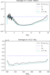 |
Fig. B.2 Computation of the radial and vertical contribution to the mass flux (Eq.B.2) compared to the measured mass flux (1.h.s. of Eq.B.2). Top panel: Temporal average. bottom panel: Spatial average. |
| In the text | |
Current usage metrics show cumulative count of Article Views (full-text article views including HTML views, PDF and ePub downloads, according to the available data) and Abstracts Views on Vision4Press platform.
Data correspond to usage on the plateform after 2015. The current usage metrics is available 48-96 hours after online publication and is updated daily on week days.
Initial download of the metrics may take a while.