| Issue |
A&A
Volume 702, October 2025
|
|
|---|---|---|
| Article Number | A80 | |
| Number of page(s) | 14 | |
| Section | Stellar structure and evolution | |
| DOI | https://doi.org/10.1051/0004-6361/202555480 | |
| Published online | 09 October 2025 | |
Noble gases neon and argon: A role for the chemical patterns of multiple populations in globular clusters?
1
Istituto Nazionale di Astrofisica – Osservatorio Astronomico di Roma, Via Frascati 33, Monte Porzio Catone I00078, Italy
2
Dipartimento di Fisica e Astronomia Augusto Righi, Università degli Studi di Bologna, Via Gobetti 93/2, 40129 Bologna, Italy
3
Istituto Nazionale di Astrofisica – Osservatorio Astronomico di Padova, Vicolo dell’Osservatorio 5, Padova I-35122, Italy
4
Dipartimento di Fisica e Astronomia “Galileo Galilei”, Univ. di Padova, Vicolo dell’Osservatorio 3, Padova I-35122, Italy
⋆ Corresponding author: This email address is being protected from spambots. You need JavaScript enabled to view it.
Received:
12
May
2025
Accepted:
4
August
2025
Abstract
Context. This paper explores the role of initial elemental abundances in the nuclosynthesis of massive asymptotic giant branch (AGB) stars and second generation abundances in globular clusters.
Aims. We look at the difficulties found with AGB models when fully reproducing the abundance patterns in second generation stars of globular clusters, and we focus on sodium destruction in models that reach the high hot bottom burning temperatures needed to efficiently cycle oxygen to nitrogen.
Methods. We built AGB models at the nominal [Fe/H] of the cluster NGC 2808. We increased the initial neon abundance by a factor of two to four with respect to the ‘standard’ abundances obtained by scaling the solar values down to the metallicity of this cluster, and explored the average abundances in the ejecta obtained by adopting smaller mass-loss rates.
Results. Higher neon produces higher sodium in the AGB envelope. Lowering the mass-loss rate enables reasonably large sodium abundances to be kept and the depletion of oxygen and magnesium to increase. A balance between the lower mass-loss rates and the necessity of not increasing the episodes of third dredge up too much gives a neon abundance that is larger by a factor of two and a mass-loss rate thgbt is smaller by a factor of four as the best compromise. A comparison with the abundances in NGC 2808 shows a better breement than the standard models for all the patterns of abundances, but the extreme stars (group E) cannot be explained in this way. Models with an initial mass ≥ 6.5 M⊙ for the same chemistry (super-AGBs) are closer to the E data, but the oxygen depletion remains too small. We also computed models slightly less rich in iron, and show that the super-AGB ejecta composition becomes more compatible with the data. Thus, we propose that the extreme population in NGC 2808 is composed of stars that have a slightly smaller metallicity, and we sketch a possible scenario for its formation within the framework of the hierarchical clusters assembly scenario. Finally, abundances of potassium are larger by ∼0.2 dex in the E group. An explanation in terms of burning of the initial argon requires a drastic increase of the relevant cross section that is similar to the adjustment required in the exploratory models for cluster NGC 2419, but it becomes easier when we assume a larger initial argon abundance.
Conclusions. The abundances of the noble gases neon and argon at low metallicities may be an important tool to better reproduce the abundances of light elements in the framework of the AGB model for globular clusters. The larger Ne and Ar abundances we need may either be a plain consequence of the uncertainties in the solar abundances of these elements or in part arise from an incomplete summing up of the sources for their nucleosynthesis at low metallicity. Thus we launch a plea for a better understanding of their galactic chemical evolution of noble gases.
Key words: stars: atmospheres / brown dwarfs / stars: evolution / Hertzsprung-Russell and C-M diagrams / stars: luminosity function / mass function / globular clusters: general
© The Authors 2025
 Open Access article, published by EDP Sciences, under the terms of the Creative Commons Attribution License (https://creativecommons.org/licenses/by/4.0), which permits unrestricted use, distribution, and reproduction in any medium, provided the original work is properly cited.
This article is published in open access under the Subscribe to Open model. This email address is being protected from spambots. You need JavaScript enabled to view it. to support open access publication.
1. Introduction
Our knowledge about the evolution of the abundances of elements in the Universe comes first of all from studying the chemical composition in the atmospheres of stars of different metallicities and relating that composition to the chemistry of the forming gas. By observing stars of different ages and chemistry, we can build a general framework to understand the chemical evolution of elements throughout the lifetime of the Universe, taking into account the nucleosynthesis in supernovae and other element factories such as s-process sites. The main standard reference for this approach is the Sun, whose abundances come in part from the study of the solar photospheric spectrum1 and in part from the analysis of meteorites. Atmospheric solar abundances agree within 10% with those in CI-type carbonaceous meteorites when normalized to the same scale (Lodders 2003). Unfortunately, meteorites are depleted in the elements that readily form gaseous compounds, like H, C, N, O, and the noble gases.
For these elements, we can only rely upon the atmospheric abundances. In regard to neon, in the solar corona we measure its abundance ratio to oxygen or magnesium, while the abundances of these latter elements are determined from the atmospheric lines. This introduces an uncertainty, a problem that was fully appreciated when the revision of the solar abundances (Asplund et al. 2006) provoked a disagreement over the helioseismological determinations of the solar properties, mainly the depth of the convective solar envelope and the inferred surface abundance of helium, (Bahcall et al. 2005a), which had been well matched by the previously adopted abundances by Grevesse & Sauval (1998). Among the many models explored to retrieve a good match for the helioseismic solar parameters, Bahcall et al. (2005b) proposed raising the neon abundance by 0.4–0.6 dex. Along similar lines, Drake & Testa (2005) derived a number ratio Ne/O = 0.41 directly from the fluxes of O and Ne in the X-ray spectra of the coronae of cool stars within 100 pc, and this value is a factor of 2.5 larger than the number ratio Ne/O = 0.15 of the solar abundances. In more recent research on solar abundances, oxygen values have been found to be not as low as in the Asplund et al. (2006) determination (see e.g. Grevesse et al. 2011), but helioseismology still requires adjustments to correctly reproduce the Sun. The approach is now to explore several different uncertain parameters (e.g. Villante & Serenelli 2020), and an increase by a factor of ∼2 in the neon abundance is still required for a good fit. Another constraint from the seismic inversion comes from the synthesis of the adiabatic exponent Γ1 profile, which is quite sensitive to the ionization of heavy elements. Using this method, Baturin et al. (2024) derive oxygen and carbon abundances that are consistent with the values by Asplund et al. (2021) and a neon abundance that is ∼20% larger, for the solar convection zone. Other abundance adjustments have emerged in recent years. The ratio of Ne/O in the transition region of the quiet Sun was increased by Young (2018) from the previous ratio, which implies an increase by 40% (with respect to Asplund et al. 2009) in the photospheric abundance of neon. An updated discussion on the uncertainties is given in Asplund et al. (2021) and Lodders et al. (2025).
We shift our attention to the abundances of the stars in globular clusters (GCs). Two main parameters characterize their chemical composition: the ‘metallicity’ (and mainly the iron content, which testifies to their chemical enrichment by supernovae) and the α-elements abundances relative to iron (which are larger than solar in the low metallicity environment and in GCs, as expected based on the prevalence of core collapse supernovae nucleosynthesis during the first phases, see e.g. Matteucci & Greggio 1986).
Historically described as ‘single stellar populations’, made up of stars that share a single age and the same chemical composition, GCs hide multiple populations. In all clusters (exceptions have been very rare until today), the majority of stars show evidence of matter processed at high temperatures by p-capture reactions; the rest are similar to field stars of the same metallicity. This apparently simple subdivision hides the complexity of the problem. If we assume that the p-capture reactions took place in a previous stellar environment, named ‘first generation’ (1G), the result is that 60–80% of the stars are ‘second generation’ (2G). Thus the 1G is deceiving us, as we no longer see it in the same place, either because it belonged to a much wider system than the cluster (e.g. for a cluster forming in a dwarf galaxy now dispersed) or because the majority of the 1G stars escaped the cluster. In addition, there is a great variety in the number of populations and in the complexity of chemical patterns (some clusters also display multiplicity in iron abundance) and any model devised should allow for this complexity in a natural way. As a general reference to the framework of multiple populations, see the recent review papers by Gratton et al. (2019), Milone & Marino (2022) and the vast literature quoted therein. In conclusion, in GCs we face a very rapid chemical evolution that took place in the very first phases of the life of globular clusters, and this requires pollution modalities very different from the chemical evolution models that account for the secular evolution of the elements during the lifetime of the Galaxy, for example the increase in iron and other elements from the population II to the solar abundances (and beyond). The latter models calibrate parameters and sometimes adopt educated guesses on the influence of different polluters to reproduce the galactic abundance trends. No model is able to fully account for the chemistry of 2G stars. In particular, the asymptotic giant branch (AGB) model (originally presented in its modern version in Ventura et al. 2001; D’Ercole et al. 2008) has been explored in much more detail than the others and is the model most subject to criticism thanks to its more detailed predictions. In spite of its fundamental advantages, not shared by any of the other models proposed so far, chemistry is the major problem of the AGB model because it is unable to provide a full explanation of the O-Na anti-correlation. Renzini et al. (2015) examine in detail how the relative roles of the cross sections of p-captures on oxygen (fluorine) and on sodium (to neon) are difficult to reconcile with the need for strong oxygen depletion and sodium survival. The most extreme stars in clusters like the prototype NGC 2808 exhibit a depletion of the surface oxygen by more than a decade with respect to first generation stars, so both burning temperatures and timescales must be large and long enough to convert a great fraction of oxygen into fluorine but p-captures deplete the sodium too, while observations show that these stars preserve a sodium overabundance.
In this paper we explore the possible role of the initial neon abundance on the chemical composition of the ejecta of massive AGB and super-AGB stars to understand whether this input can improve the comparison with the composition found in 2G stars. Our starting point follows the idea that the solar neon abundance is underestimated by a factor of two to four, so that the neon abundance at the smaller metallicities of GCs is also underestimated by the same factor. The neon increase we propose is additional to the α-enhancement factor already taken into account when scaling the neon abundances. In our conclusion, we consider a factor of two increase to be the best compromise. A different interpretation of this approach is to consider the solar neon abundance to be correct, and assume that neon, at lower metallicities, was indeed more abundant than suggested by scaling. Unfortunately, the scarce present day neon abundance determination in planetary nebulae (see Sect. 7 and Fig. 6) does not help us determine the more plausible choice.
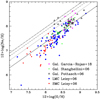 |
Fig. 6. Schematic neon versus oxygen abundances in planetary nebulae. The solar point is located at the abundances from Lodders (2003). The diagonal lines show the location for solar-scaled abundances (full line) and for neon abundances twice (dots), three times (dashed), and four times (dot-dashed) the solar value. Data are taken from different sources for planetary nebulae, as labelled. |
In Sect. 2 we briefly outline the main accomplishments and in Sect. 3 we recall the main difficulties of the AGB model when accounting for the chemistry of 2G stars. In Sect. 4 we present models with reduced mass-loss rates and enhanced neon that aim to explain the different populations found in NGC 2808, one of the GCs that shows the most extreme anti-correlation of light elements and that has been well studied for many different elements; we also explore models with a slightly smaller iron content and show that their ejecta composition better matches the abundances most extreme stars of the cluster. In Sect. 5 we propose a formation model for NGC 2808 that may account for the extension of all the anti-correlations. In Sect. 6 we discuss preliminary models to synthetize potassium and in Sect. 7 we briefly discuss the neon abundances in planetary nebulae. Although the results presented in this work are in the right direction, solving the several open problems requires careful adjustment of the inputs.
2. The AGB model
Although many factors related to a cluster’s internal dynamics and its complex interplay with the external galactic environment (particularly in the early stages of galaxy formation) certainly play a key role in determining the current properties of multiple-population clusters, any effort aimed at identifying the fundamental ingredients in the formation of multiple populations should be driven by the strong observational constraints that come from the chemical abundance properties and patterns revealed by spectroscopic and photometric observations. We need to identify which are the fundamental clues to the possible sources of gas out of which 2G stars formed. In brief, the strongest chemistry constraints we must deal with are thefollowing.
-
The inner helium content of 2G stars is larger – generally moderately larger – than the helium content of 1G stars but it appears to be limited to a maximum mass fraction Y ≃ 0.35–0.38, with such large abundances found only in a fewclusters.
-
The typical anti-correlations found in the abundances of p-capture elements (C-N, N-O, Na-O, and Na-Al) are common in all clusters; some clusters also show Mg-Al and Mg-Si anti-correlations.
-
Very few clusters show a potassium versus magnesium anti-correlation, and possibly a mild correlation of K-Ca.
The increase in helium content is to be expected, as we are dealing with hydrogen burning, and the existence of an upper limit is an important clue. Increasingly high temperatures are required to account for the p-captures that are at the basis of the different anti-correlations. The main cycles of p-captures are shown in Fig. 1, where the temperatures necessary for the activation of the cycles are ∼20 MK for the CN cycle (yellow box in the bottom panel) and ∼40 MK for the NO cycle (green box). The 24Mg, which is manufactured by He-burning reactions in the massive star progenitors of the cloud that forms the 1G stars, can only be subject to p-captures at the base of the convective envelope for temperatures larger than 100 MK, and in a few cases the p-capture chain may extend to Al, increasing Si (see Fig. 1). Temperatures as high as 100 MK are not reached in the centre of regular massive stars2. This led to the selection of supermassive stars as a possible processing site (Denissenkov & Hartwick 2014). In spite of the high temperature nuclear processing in the gas now forming the 2G stars, the fragile element lithium is preserved, with abundances close to standard, or is only partially depleted in stars that show the most extreme anti-correlations.
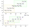 |
Fig. 1. Schematic p-captures for the CN (yellow box) and NO (green box) cycles (bottom panel) and for the Ne-Na (yellow) and Mg-Al and Al-Si (green) cycles (top panel). Blue arrows indicate (p,γ) reactions, pink trajectories indicate p-captures followed by β decays, dashed red lines show (p, α) reactions. The processing occurs for increasing hot bottom burning temperatures. |
In the models most extensively studied in detail, p-captures do not take place in the stellar cores, but at the basis of the convective envelopes of massive AGB stars, where the temperature at the bottom (THBB) becomes so high that the elements are subject to ‘hot bottom burning’ (HBB, Boothroyd et al. 1993). During the AGB evolution, the processed gas is transported by turbulence to the surface of the AGB and is lost into the outer space by stellar winds and planetary nebula ejection. This phase is short-lived, and the temperatures of HBB depend on the model adopted to describe convection. However, the most massive and very low metallicity models that employ highly efficient convection may achieve extremely high temperatures (120–130 MK). In these conditions, p-captures on argon may occur, which may explain the potassium overabundances reported above (Ventura et al. 2012).
O-depletion in the massive AGB envelopes of low metallicity stars subject to HBB was first extensively found in the models built by Ventura et al. (2001). At the time, no other stellar models confirmed these results. Two main physical inputs were the reason for the big difference in the new results:
-
The convection model: all the other models employed the standard mixing-length theory (Böhm-Vitense 1958), and the efficiency parameter was generally left at the value obtained (at that time) to fit the solar model. The new models by Ventura et al. (2001) employed the full spectrum of turbulence (FST) model (Canuto & Mazzitelli 1991; Canuto et al. 1996). This choice resulted in a higher convection efficiency at the bottom of the convective envelope of AGB models, which produced two main effects: (1) a shorter distance between the outer edge of the CNO-burning shell and the base of the convective envelope, which increased the efficiency of the HBB p-capture reactions. The products of these reactions were transported throughout the convective envelope and finally ejected to the interstellar medium; (2) extra-luminosity, which triggered a faster growth of the stellar luminosity and hence of mass-loss rates (Ventura & D’Antona 2005a).
-
The mass-loss treatment: we adopted the Bloecker (1995) formulation for the mass-loss rate:
 (1)
(1)where M and L are the stellar mass and luminosity, and ṀR is Reimer’s mass-loss rate, depending on the stellar radius R (all given in solar units):
 (2)
(2)The parameter η in our models has been calibrated on the statistics of lithium rich giants in the Magellanic Clouds (Ventura et al. 2000) to η = 0.01 − 0.02. Such a mass-loss rate, which is dependent on a high power of the luminosity, together with the effect of the efficient convection reduce the overall duration of the AGB evolution by a factor of approximately three with respect to solar-calibrated mixing length theory (MLT) computations3, thus enhancing the mass loss during the phases of maximum Na production and reducing the mass lost when Na was depleted in the envelope (Ventura & D’Antona 2005b). In addition, Ventura & D’Antona (2006, 2009) selected the most favourable range allowed for the cross sections of the NeNa-cycle reactions (considering the existing uncertainties) and maintained the Na abundances that conform to the observational data.
To summarize, by choosing the most efficient convection model available (the FST), by tuning the mass-loss rate to values compatible with the analysis of the lithium-rich giants in the Magellanic Clouds, and by tuning the cross sections of the NeNa-cycle reactions, the ejecta of massive AGB stars showed both oxygen depletion and preservation of sodium at levels compatible with the observed Na-O anti-correlation. The AGB model is able to account for a good number of the features of GCs. In particular, stellar models and dynamical models have been studied in detail and provide a reasonable match to the complexity and variety of chemical patterns in the multiple populations. The long evolutionary times of AGB masses give long timescales for the formation of the 2G stars and easily account for different chemical pollution patterns that follow the different structures of AGB of different mass (D’Antona et al. 2016).
3. The pro and cons of the AGB model
The most critical aspect of the AGB model is illustrated in Fig. 2, which shows the evolution of the surface mass fractions of sodium and oxygen with time, along the AGB phase of 6 M⊙ model stars, calculated with different initial neon abundances. The depletion of sodium necessarily accompanies the depletion of oxygen during the AGB evolution because the cross section for p-captures on 23Na nuclei is larger than the cross section for p-captures on 16O nuclei (see e.g. Renzini et al. 2015, for a discussion). Thus, when oxygen burns, sodium also burns. Sodium may preserve an average abundance higher than in the first generation only because the second dredge-up has replenished the envelope with sodium and neon from the helium intershell, and neon has been rapidly converted to sodium thanks to the high THBB. Even if sodium and oxygen are both burned in the following AGB evolution, the average abundance of sodium in the ejecta may remain large.
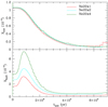 |
Fig. 2. Changes of the sodium abundance versus time for the 6 M⊙ AGB evolution, when we vary the Ne20 initial abundance in the models. For simplicity, we show models with the same mass-loss rate calibration η = 0.002, that is 1/10 of the standard value η = 0.02. |
3.1. The comparison cluster: NGC 2808
All comparisons are made with the abundance patterns in NGC 2808. The choice is well motivated but also needs justification. It is a standard result of AGB evolution that the temperature (THBB) at the base of the convective envelope for a given mass increases for lower metallicities, corresponding to lower opacities of the envelope matter. Stars in NGC 2808 have a relatively high metallicity ([Fe/H] = –1.1, Carretta 2015) but in spite of this they display very extended abundance patterns; as a consequence, NGC 2808 is an important benchmark for any new modelling. In addition, the stars also show a spread by a factor of ∼2 in the abundances of potassium (Mucciarelli et al. 2015), although this element is only seen to vary mainly (by an entire decade) in the very low metallicity cluster NGC 2419 (Cohen & Kirby 2012)4. Although it was not revealed in the spectroscopic analysis, it is possible that the 1G stars of NGC 2808 display a moderate metal inhomogeneity, δ[Fe/H] = 0.25±0.06 dex (Lardo et al. 2022).
The accurate catalogue of abundances in Carretta (2015), subdivided into five subgroups of increasing chemical ‘anomalies’, constitutes the most complete spectroscopic benchmark we must comply with, and the abundances are shown in Figs. 3 and 4. The stars were assigned to the P1, P2, I1, I2, and E classes based on their location in the Mg-Na plot, where the groups are well distinguished. The discreteness of the groups is a significant hint that the formation of the multiple populations occurred in bursts, and probably from matter contaminated by polluters in which the gas was processed by p-captures at different temperatures. In the AGB model, this is a very probable situation (D’Antona et al. 2016) because the second generation formation occurs on a long timescale of several tens of million years, as modelled by D’Ercole et al. (2008, 2016), Calura et al. (2019). We can take this into account when we compare the data with the new exploratory models.
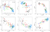 |
Fig. 3. Anticorrelations of p-capture elements in the GC NGC 2808 (Carretta 2015). The diagram of sodium-magnesium data (panel b) was the basis for the subdivision into different sub-classes: P1 (blue), P2 (green), I1 (red), I2 (orange) and E (black). All panels show: (1) standard average abundances in the AGB ejecta by for a metallicity Z = 2.3 × 10⁻³, [α/Fe] = 0.4, e.g. [Fe/H] = –1.08 (open blue circles); (2) exploratory models (coloured squares and connecting lines) with the same initial composition and identified by the following. GREEN: Ejecta of the 6 M⊙, with standard neon and decreasing mass-loss rates (models ηxNe1). Starting from the standard abundances for η = 0.02, we plot η = 0.01 (1/2 standard), 0.005 (1/4 standard), and 0.002 (1/10 standard); BLUE: 6 M⊙ for η = 1/10 standard, with increasing neon abundance from standard (solar scaled, for α/Fe = 0.4) to two and four times standard (models η 0.1Ne4); RED: Abundances for the 5 and 7 M⊙ for η 0.1Ne4; CYAN: Starting from mass loss 1/4 standard, and increasing neon at two and four times the standard abundance (models η 0.25Ne2 and η 0.25Ne4). The big blue and cyan stars define the location of the models that have sodium consistent with the O-Na patterns and discussed in the text: η 0.1Ne4 and η 0.25Ne2, which we will also consider in the other panels. The dark grey lines with triangles define dilution of the 6 M⊙ location η 0.25Ne4 with increasing quantities (20, 40, 60 and 80%) of gas with standard composition, identified by the yellow star. |
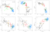 |
Fig. 4. Same as Fig. 3, showing different model outputs. GREY: The squares represents the 5.5, 6.5, 7, and 7.5 M⊙ location for the new standard η 0.25Ne2; BLACK: (Open black squares) models η 0.25Ne2 for 5.5, 6, 6.5, and 7 M⊙, for models that have δ[Fe/H] = –0.1. The big cyan stars define the location of the new standard, η 0.25Ne2, 6 M⊙. In panel a, the green squares are the 6 M⊙ ejecta for mass-loss rates with Reimers’ parameter η going from η = 0.001 (0.1 standard) to η = 0.02 (old standard), also shown in Fig. 3. |
3.2. Abundances in the standard models
In our first comparisons with the abundance patterns of NGC 2808, we used models with a metals mass fraction of Z = 0.001, where the elemental abundance ratios followed the Grevesse & Sauval (1998) abundance distribution. In the following the solar abundances were revised and it became clear that the HBB depends on the opacity of the envelope, which is dictated by the iron abundance more than by the total metallicity. It is necessary to update our comparisons and take into account the specific abundances and abundance ratios more strictly. In the present models, our standard mixture follows Asplund et al. (2009), where the percentage of neon is 0.094 and Z⊙ = 0.014. The solar mass fraction of neon is then ZNe = 1.31 × 10⁻³. For NGC 2808 we adopt [α/Fe] = 0.4, so that the standard neon fraction becomes 0.1208 of the total metallicity, fixed at Z = 2.3 × 10⁻³. Thus the neon mass fraction in the standard models is 2.78 × 10⁻⁴. When we define models with a factor of x2 or x4 neon, we mean this mass fraction is multiplied by two or four, while the other abundances remain the same (in particular [Fe/H]). With this choice, the total metallicity Z increases and the fractional values of the other abundances readjust.
3.3. Standard models do not deplete enough oxygen
The Na and O average abundances in the ejecta for different AGB masses are seen as blue open circles in panel a of Fig. 3. The results refer to models of [Fe/H] = –1.08 [α/Fe] = 0.4 for a total metallicity of Z = 2.3 × 10⁻³. The details of the input physics of the models are given in Dell’Agli et al. (2018) and the mass-loss rate follows the Bloecker (1995) formulation (see eqs. 1 and 2) with η = 0.02. The iron content of these models is very close to the value determined for NGC 2808, whose abundance patterns are displayed in the panels of the figure. We see that oxygen in the models does not match the I2 or the E group, as its maximum depletion, starting from an initial abundance of [O/Fe] = 0.4, is ∼0.55 dex for the 5.5 M⊙. Previous comparisons with NGC 2808 (e.g. D’Antona et al. 2016) were based on models by Ventura et al. (2013) computed for a lower metallicity (Z = 10−3), for which p-processing is stronger and therefore shows a greater oxygen depletion (∼0.8 dex for the 6 M⊙ models), although not sufficient to match the E subclass.
It is important to mention the typical ‘hook’ shape of the O-Na ejecta abundances as a function of the mass. The average abundances in the ejecta depend on the interplay between two main parameters of the models: THBB and the mass-loss rate. Oxygen burning will be more effective the higher the THBB and the lower the mass-loss rate. Both these quantities increase with the evolving mass; higher mass models have larger luminosities, larger mass-loss rates, and consequently shorter AGB evolution so the oxygen has less time to be converted into nitrogen by HBB. The oxygen depletion first increases with decreasing mass, until the lower THBB prevails and oxygen increases again in the ejecta. There is a ‘turning mass’, typically in the 5 − 6 M⊙ range (Dell’Agli et al. 2018), for which a minimum oxygen abundance is reached, and it is higher for lower metallicity and has a higher THBB. Lower mass-loss rates for the same physical inputs produce a higher oxygen depletion. Instead, the sodium abundance in the ejecta is mainly connected to the rapidity of loss of the envelope, so it is higher for a higher initial mass, then increases again when the third dredge up starts to be effective.
For the compositio of the models on display, the oxygen abundance in the ejecta is first correlated with the stellar mass and decreases, going down from 7 to 5.5 M⊙. Decreasing the mass further, from 5.5 to 4.5 M⊙, another effect becomes dominant; the AGB phase lasts longer (thanks to the lower luminosity and mass-loss rates) and the third dredge up episodes noticeably alter the envelope composition by increasing the total CNO, because 22Ne is also dredged up from the helium intershell and is immediately converted into sodium by p-captures. Thus the sodium abundance increases. As the total CNO is approximately constant in 2G stars, and sodium is not as large as predicted by models that have M ≲ 4.5 M⊙, the 7–5 M⊙ range is the best for producing 2G stars. In summary, the resulting composition of the ejecta is a complex result of the choice of convection model (temperature of HBB) and mass-loss law.
3.4. Extreme stars with oxygen abundances lower than allowed by models
The comparison (Fig. 3, panel a) between the O-Na of the ejecta of the models (open blue circles) and the data for NGC 2808 shows that both the ‘intermediate’ I2 (orange dots) and the ‘extreme’ E stars (black dots) of the cluster have an oxygen abundance up to 0.5–0.7 dex smaller than modelled. As all these stars are giants, this discrepancy can be explained by the fact that the extreme abundances go together with ‘pure’ (undiluted) AGB ejecta, which also have a very high helium abundance (Y ∼ 0.35–0.36, Ventura 2010), and are also more easily subject to extra mixing as they develop a much smaller molecular weight barrier (D’Antona & Ventura 2007); as a consequence, these stars may lower their atmospheric [O/Fe] during the red giant branch evolution. The extra mixing depletes oxygen but not sodium, so O and Na both fit the observed values. This escape requires ad hoc modelling if it is not limited to suggest an additional depletion by 0.1–0.2 dex, but instead implies a factor of two to three reduction in the oxygen abundance. Furthermore, and possibly more directly relevant, we have to assume that all the I2 and E stars have been born from pure AGB ejecta, with a helium content in the range of Y = 0.35–0.36. This may be consistent with the data for the cluster NGC 2808: its colour magnitude diagram shows the presence of a blue main sequence that corresponds to a high helium content (D’Antona et al. 2005; Piotto et al. 2007; Milone et al. 2015), and spectroscopically its ‘extreme’ population E shows the largest oxygen depletion, magnesium depletion, and silicon enhancement of matter processed in very massive AGB or super-AGB stars (Carretta 2015; Milone et al. 2017; D’Antona et al. 2016). On the other hand, for example, it was clearly shown that the maximum value allowed in the ‘extreme’ stars of cluster NGC 6402 is Y ∼ 0.31, although they show oxygen abundances that correspond to the composition of pure AGB ejecta (D’Antona et al. 2022). Study of the horizontal branch morphology (Tailo et al. 2020) or of the chromosome map (Milone et al. 2017, 2018) limits the maximum helium of the 2G stars to Y = 0.30–0.31 in several clusters, which also applies for the stars that have O-Na abundances expected for the pure ejecta of the models, and these have much larger helium, Y ∼ 0.35 (e.g. D’Antona et al. 2022). The problem of discrepant helium abundances was first pointed out by Bastian et al. (2015) by considering the helium contents predicted by models for samples of stars with limited oxygen depletions. The way out of this conundrum requires models to destroy more oxygen during the AGB evolution so that the O-Na anti-correlation requires dilution with a larger quantity of pristine gas, which also lowers the helium abundance in 2G stars (see Fig. 13 in D’Antona et al. 2022). Incidentally, we note that a larger dilution may be in better agreement with the lithium abundances in 2G stars, independently of the lithium produced during the AGB evolution (D’Antona et al. 2019). Thus it is possible that extra mixing in high helium stars is taking place, but its role must have a limited effect (∼0.2 dex) on the oxygen extra depletion.
In regard to the other light elements, the problem is only present for the limited number of clusters that also show Mg depletion and Si increase. A better agreement for Mg and Si requires longer timescales of evolution and HBB burning. In general, we need a longer AGB phase, which can be obtained by reducing the mass-loss rate, to fit better the O and Mg depletion and the Si increase. The undesired effect is to strongly deplete Na too, in disagreement with the observations.
In the following we discuss the AGB models by our group published so far. We focus on the other p-capture elements and the other points of weakness of these models.
3.5. Magnesium depletion, Mg-Si anti-correlation, and magnesium isotopes ratios
In a fraction of clusters, Mg also shows abundance differences between 1G and 2G stars. In the AGB model, this implies that in some clusters HBB occurs at higher temperatures than in others. Mg depletion is especially seen in low metallicity clusters and this is consistent with the fact that HBB temperatures are larger in models with lower envelope opacities. An example of the trend of models and data with metallicity is provided in Ventura et al. (2018) (see in particular their Fig. 6). The best evidence is given by the observations of Mg abundances in ω Cen (Mészáros et al. 2015; Alvarez Garay et al. 2024), where only the lower metallicity populations show Mg depletion. In this work, Alvarez Garay et al. (2024) also show the presence in ω Cen of a Mg-Si anti-correlation, which indicates that the Mg-Al cycle is extended to the 27Al(p,γ)28Si reaction (see Fig. 1). The ‘standard’ models built for NGC 2808 do not account for the high spread shown by Mg and Si in this cluster (see the relevant panels in Fig. 3).
3.6. The potassium versus magnesium anti-correlation and its extent
The abundance of potassium in the 1G stars results from the nucleosynthesis in core collapse supernovae, whose uncertainties or metallicity dependence is still under investigation (e.g. Kobayashi et al. 2011). However, it was surprising to find a variation by a factor of ten in its abundance, anti-correlated with magnesium abundance, among the red giants of the metal poor cluster NGC 2419 (Cohen & Kirby 2012; Mucciarelli et al. 2012). As the magnesium depletion in the 2G stars implies that their gas had been processed at very high temperatures (≳100 MK), Ventura et al. (2012) proposed that p-captures, at even larger temperatures, also manufacture potassium. In fact the cross sections of the chain 36Ar(p,γ)37K(e+,ν)37Cl(p,γ)38Ar(p, γ)39K increase by orders of magnitude at temperatures above 100 MK. In super-AGB models, Ventura et al. (2012) were able to achieve HBB temperatures THBB ∼ 120 MK and K production was obtained by increasing the cross section of the reaction 38Ar(p,γ)39K by a factor of 100.
At present, only three clusters5 are recognized to have a potassium spread that is anti-correlated with magnesium or oxygen: NGC 2419, NGC 2808 (Mucciarelli et al. 2015), and ω Cen (Alvarez Garay et al. 2022). As we have pointed out for neon, the abundances of the noble gas 36Ar (an α-nucleus that will be the most abundant form of argon at such low metallicities) and of the other argon isotopes are also not well known.
4. An uncommon player: The initial neon abundance in the first generation gas
As shown in Fig. 2, the ‘second dredge-up’ that occurrs at the beginning of the AGB evolution not only affects the helium abundance (Ventura 2010) but also the sodium and the neon isotopes processed in the interior. Fast p-captures on the dredged-up neon contribute to increase sodium during the first phases of HBB (Ventura & D’Antona 2005a; Ventura & D’Antona 2005b).
As HBB progresses, sodium is gradually destroyed. Therefore, the average sodium abundance in the stellar ejecta depends on the balance between the mass lost during the early phase (when sodium is enhanced due to second dredge-up and p-captures) and the mass lost later, when sodium has already been depleted.
In the meantime, the NO cycle continues to operate on the oxygen abundance, which remains at very low nuclear equilibrium values. For this reason, if we lengthen the AGB evolution and slow down the mass loss, we achieve a lower average oxygen, but also a lower average sodium abundance.
Based on the above discussion, it is not possible to sufficiently reduce oxygen without simultaneously destroying an excessive amount of sodium, if we assume standard initial abundances. However, if the initial neon abundance is higher than assumed in standard compositions, the initially higher peak of dredged-up neon converted into sodium helps to counteract the decrease in average sodium in the ejecta. Thus it is worth looking in more detail at models with increased initial neon.
4.1. Role of the mass-loss rate and neon abundance
The top left panel of Fig. 3 shows the ‘standard’ models (η = 0.02) for [Fe/H] = –1.08 and for AGB masses from 7 to 4.5 M⊙. We take as reference the 6 M⊙ model, and show the abundances obtained by reducing η by a factor of two, four, and ten: the abundances (green squares) shift to lower oxygen and, obviously, to lower sodium for the reasons outlined in Sect. 3. Oxygen is depleted by a factor of ten in the model with the lowest mass-loss rate. Starting from this model location, we can recover a high sodium abundance if we increase the initial neon abundance: the blue square and the big blue stars show the results obtained by multiplying the initial neon by a factor of two and four, respectively. The last model comes back to the range observed for the range of sodium abundance. We identify specific models by their η reduction x and neon increase y as ‘η x Ne y’. If we increase the Ne abundance in the model with η = 0.005 by a factor of two and four, we reach the locations of the big cyan asterisk and cyan square. Two ‘dilution curves’ (grey lines) between the Na-O abundances in the models η 0.1Ne4 and η 0.25Ne2 and the initial abundances (big yellow star) are drawn. The triangles along the lines represent the dilution of AGB ejecta with 20, 40, 60, and 80% pristine gas.
4.2. Discussion of the results: The most appealing compromise
In Fig. 3 we compare the abundances of NGC 2808 and the model predictions in the planes Na versus O (panel a), Mg versus Na (panel b), Al versus Mg, (panel c) Si versus Mg (panel d), Si versus O (panel e), and Mg versus O (panel f), with special attention both on the η 0.1Ne4 (big blue star) 6 M⊙ and on the η 0.25Ne2 (cyan star) results. Panel a of Fig. 3 shows that the 6 M⊙ AGB ejecta of model η 0.1Ne4, diluted with pristine gas, can be representative of the 2G stars in NGC 2808, apart from a very few E stars (black dots), for which we can still invoke some extra mixing during the giant branch evolution of these high-helium stars, as discussed in Sect. 3.4. Panel b shows that the Mg abundances of the I2 group are well reproduced by the same model, while the evolution of the 7 M⊙ is able to reproduce the Mg of the E group. A similar good agreement is found for Al (panel c) and Si (panel d). Unfortunately, the mass-loss rates in models η 0.1Ne4 are so low that the 5 M⊙ evolution already begins to be significantly affected by the third dredge-up. While it fits (top red square) the Na-O abundances of the E stars very well, its C+N+O abundance would be about 1.7 times larger than the initial CNO, at the limit of what is allowed from observations (Carretta et al. 2005)6. In addition to the problem of CNO abundances, it is hard to invoke an increase of neon by a factor of four (see Sect. 7).
The η 0.25Ne2 model (cyan star) of 6 M⊙ has Na and O compatible with the observed abundances. Oxygen is reduced by 0.8 dex and only leaves out the extreme E stars. An increase by a factor of two for neon is more reasonable, so η 0.25Ne2 is the best compromise for the 2G stars, but it does not explain the extreme stars in group E.
Panel b of Fig. 3 shows that progressively reducing the mass-loss rate leads to lower abundances in the ejecta, as proton-capture reactions on both oxygen and magnesium have more time to operate. The increase in neon has a small or negligible effect on the final abundances. In any case, the Mg depletion does not increase enough to reach the E sample location. Lower mass-loss rates lead to a better representation of the Al production (panel c) although for this element too the abundances in the E stars is a bit larger, by ∼0.1 dex, and is not even reproduced by the 7 M⊙ evolution. The discrepancy is very small, considering that the range of variation in Al is ∼1.5 dex. Similarly, both Mg and O of group E are not explained (panel f), and the extension in Si abundances is not met (panels d and e) although the model location with lower mass-loss rates is largely improved.
In conclusion, the position of the blue and cyan asterisks in the figures suggests that the location of the E group (blue asterisk) stars is only met by assuming a very low mass-loss rate (1/10 of the ‘standard’ rate adopted in all our previous models published so far) and a very high neon increase (four times larger than the solar standard abundance adopted today). Both these choices are biased; a low mass-loss rate is only compatible with the 2G chemical patterns if the ejecta from stars near 5 M⊙ contribute very mildly to 2G formation. This significantly narrows the viable mass range to approximately > 5–7 M⊙ thereby exacerbating the mass budget problem. Furthermore, such a large neon abundance is not compatible with the observational data (see Sect. 7). The more modest increase in neon (two times) and the more conservative reduction by a factor of five in the mass-loss rate (η = 0.005) provides a good representation of the NGC 2808 groups of abundances, apart from group E. Therefore, an alternative mechanism must be operating and requires further investigation to fully account for the characteristics of class E.
4.3. Models with reduced [Fe/H]
Figure 4 shows the average abundance in the ejecta of models for the case η 0.25Ne2 and several different masses: 5.5, 6 (the standard case), 6.5, 7, and 7.5 M⊙. The abundances of group I2 are better explained when we consider the role of different masses, while the E stars are still problematic.
We therefore considered the abundances of ejecta for a chemical composition in which the iron content is reduced by δ[Fe/H] = –0.1. Although in general the mass-loss rate may be dependent on the metallicity, such a small change allows us to leave the mass loss parametrization unchanged at the value η = 0.005. The results are plotted as open black squares and, interestingly, such a small abundance difference is able to shift the ‘turning’ mass (see Sect. 3.3) from 6 to 6.5 M⊙, so that depletions of larger elements are achieved and the abundances are much closer to the location of group E stars in the different panels. The iron-reduced 6.5 M⊙ performs better than the 6 M⊙ with standard iron content, and also provides results closer to the E group for Al, Si, and Mg, while it fails to fully reproduce O with a mild discrepancy (reduced to ∼0.2 dex).
5. A lower [Fe/H] for the E population: A proposal for the cluster formation
We conclude that group E abundances are consistent with the AGB model if the AGB progenitors of this group have a slightly smaller metallicity than the bulk of other stars. The F275W−F814W colour spread of 1G stars in the pseudo two-colour diagram – known as the chromosome map (ChM) – indicates that the 1G population of NGC 2808 is not chemically homogeneous. Instead, it exhibits a metallicity spread of approximately [Fe/H] ∼ 0.1 − 0.2 dex (Milone et al. 2015; D’Antona et al. 2016). In particular, a comparison between the observed colour distribution of 1G stars in NGC 2808 and synthetic colours from isochrones with varying metallicities suggests that the range between the 90th and 10th percentiles in the iron abundance distribution corresponds to 0.11 ± 0.01 dex (Legnardi et al. 2022).
Supporting this, a differential analysis of high-resolution spectra for five stars spanning the 1G sequence on the ChM, conducted by Lardo et al. (2022), reveals a maximum iron variation of 0.25 ± 0.06 dex. These moderate iron variations had not been detected in earlier studies based on absolute spectroscopic measurements (e.g. Carretta 2015). Thus such a iron spread was present at the formation of the 1G, or possibly it was introduced while the cluster stars were already forming (Lardo et al. 2023).
The formation of NGC 2808 might have followed the root of hierarchical merging of different initial independent star-forming clumps into a single massive cluster. This model has received attention in recent years thanks to observations showing that young stellar systems often have a complex clumpy structure consisting of several stellar sub-systems (e.g. Kuhn et al. 2020; Lim et al. 2020; Dalessandro et al. 2021a,b). Some of these agglomerates may finally dissolve but some of them may evolve into more massive stable clusters (Dalessandro et al. 2021b; Della Croce et al. 2023) and, as shown by simulations, eventually hierachically merge into a single massive cluster (Livernois et al. 2021). Attempts to link this merging to the multiple populations present in GCs – mainly concerning either age differences or the multiple iron abundance clusters – have been made by Gavagnin et al. (2016), Hong et al. (2017), Bailin (2018).
We can assume that the E population is the second generation formed from the high mass AGB and super-AGB stars evolving in a massive clump that first formed stars. The other clumps started star formation later and their gas was polluted by the core collapse supernovae exploding in the first clump (e.g. Bailin 2018), so the stars formed in the other clumps were more metal rich. While the different clusters were merging into the final cluster NGC 2808, the ‘first’ 2G formed in the cooling flow of the high-mass AGB of the first more metal-poor cluster. To reproduce the abundances of group E, it is necessary that the difference in age between the age of the first clump and that of the others be larger than about the time necessary for the 6.5 M⊙ to evolve, for example ∼60 Myr, and it is also necessary that the first clumps are sufficiently massive that their pure AGB ejecta from ∼8 to ∼6.5 M⊙ are compatible with the mass of population E. When the other clumps also begin their AGB evolution, the winds from different evolving masses and different metallicities merge in the cooling flow and the metallicity is, on average, larger. The composition of population E would then be that of pure ejecta, with a high helium content Y = 0.36–0.37, which is consistent with the location of the blue main sequence of NGC 2808 (D’Antona et al. 2005; Piotto et al. 2007).
As the last supernova event occurs at ∼44 Myr, for stars above 7.5 M⊙, we need an age difference of ∼15 Myr between the birth of stars in the first clump and in the other ones. After this period, the core collapse supernova epoch ends in the other clumps, and the cooling flow onto the baricentre of the system proceeds, now including a mixture of AGB ejecta from stars with different metallicities. The mixing timescale of the gas in the cooling flow is short enough that the metallicity spread of these 2G stars is very small, as observed (Legnardi et al. 2022). Note that the mass of the clumps must be adequate to account for the present day population fraction. In particular, the stars in population E are 14% (Carretta 2015) of the total mass (M = 7.91×10⁵ M⊙, Baumgardt et al. 2019, and corresponding web page), so ∼1.1 × 10⁵ M⊙, and must have all been born from the ejecta of the AGBs between ∼7.5 and 6.5–6 M⊙. For a standard Kroupa IMF, the initial mass of the putative lower metallicity clump must then be 4 − 5 × 10⁶ M⊙, so it is the most massive of the components. We will examine the hypotheses in detail in a forthcoming paper.
6. The Potassium problem
Figure 5 shows the last chemistry issue in NGC 2808: the abundances of potassium versus oxygen and potassium versus magnesium. More than an increasing trend of K for decreasing O or Mg, the data seem better represented by a single potassium abundance for all groups, apart from the E group, showing a K abundance higher by ∼0.2 dex. We follow the idea of Ventura et al. (2012) and look at the effect of the chain 36Ar(p,γ)37K(e+,ν)37Cl(p,γ)38Ar(p, γ)39K for the production of potassium. Although 0.2 dex is not a factor as huge as the ten times increase in cluster NGC 2419 (Cohen & Kirby 2012; Mucciarelli et al. 2012), the [Fe/H] of the present models is much larger, and that of the THBB consequently smaller, so the AGB models do not show a significant K increase. Nevertheless, for the highest masses of the models with [Fe/H] reduced by 0.1 dex, and increasing the nuclear reaction rates as done for NGC 2419, some small increase in K was obtained. The increase was by 0.065 dex for the 6.5 M⊙. The initial argon abundance was kept in the solar proportion. By doubling it, the total increase in K was by 0.12 dex. We report this latter value in Fig. 5. The result is in the right direction but the requirements are so strong that it is not worth trying to achieve a better agreement. We only note that the argon abundance is a possible additional parameter to treat the problem of potassium.
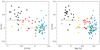 |
Fig. 5. Potassium-oxygen and potassium-magnesium data for the GC NGC 2808 (open circles) from Carretta (2015) and Mucciarelli et al. (2015). For all the symbols, see Fig. 3. Depletion for 6.5 M⊙ with [Fe/H] reduced by 0.1 dex is shown by the open squares. The upper point (δ[K/Fe] = 0.125) is obtained by doubling the argon initial abundance. See text for further information. |
7. Neon abundances in planetary nebulae
Figure 6 shows the neon versus oxygen abundances in planetary nebulae (PN), where oxygen is a proxy for metallicity and the solar point is shown at the abundances by Lodders (2003). The diagonal lines show the location for solar-scaled abundances (full line) and in the hypothesis that the solar neon abundance is twice (dots), three times (dashed), and four times (dot-dashed) the solar value. Data are taken from different sources: galactic PN from García-Rojas et al. (2018) (purple) and Stanghellini et al. (2006) (green dots), galactic PN from Pottasch & Bernard-Salas (2006), and Large and Small Magellanic Clouds PN (Leisy & Dennefeld 2006). A detailed analysis of the data is beyond the scope of this work; however, it is worth noting that several measurements show neon abundances higher than solar at oxygen levels near solar, whereas only a few low-oxygen data points exhibit super-solar neon. Additionally, data at low metallicity are scarce. While this comparison remains inconclusive, it suggests that more neon abundance measurements are needed before drawing firm conclusions about the initial neon levels in low-metallicity environments, such as those found in proto-GCs.
8. Conclusions
In this work we make two proposals to lessen the discrepancy between the AGB scenario and the distribution of the abundances of light elements among GC stars. The first proposal is to consider whether the initial neon abundance of the forming cluster can be larger. As neon is an alpha element, an α/Fe ≃ 0.2–0.4 is generally already introduced in the choice of the initial neon abundance. We now add a further increase. We follow this approach because the solar abundance of noble gases is not well known, as summarized in Sect. 1. Our comparisons are made with the data for GC NGC 2808, one of the most complex GCs for its extended light element anti-correlations, which are very well studied in the spectroscopic sample by Carretta (2015). If we limit the initial neon increase to a factor of two larger than the solar-scaled abundance, we can reduce the mass-loss rate generally adopted in the models by a factor of four and can explain better the anti-correlations, apart from the abundance values of the most extreme group of the cluster. The abundances in planetary nebulae (Sect. 7) do not contradict such a neon increase for solar metallicities, but there is too little data at the low metallicities of GCs to make a more significant comparison. An alternative possibility is to consider the solar neon and argon abundances correct, and suggest that, at low metallicity, the ratios Ne/Fe and Ar/Fe are larger than what is implied by their being α elements. We then propose that an effort be made to improve our understanding of the stellar yields of noble gases and their galactic chemical evolution.
Our second proposal is to suggest that the very high extension of the anti-correlations in the cluster NGC 2808 is ultimately due to the coexistence in the cluster of different metallicities in the 1G stars. In the framework of the hierarchical cluster assembly scenario (e.g. Della Croce et al. 2023), we show that the extreme stars in NGC 2808 are better modelled if the stars that show the most extreme anti-correlations have a metallicity smaller by 0.1 dex. As this cluster appears to have a global iron spread of ∼0.25 dex (Lardo et al. 2023) among its 1G stars, we suggest that it was formed by the assembly of multiple clumps that had slightly different metal abundances.
Finally, we try to model the potassium variations shown by the extreme stars, in the framework of the explanations proposed by Ventura et al. (2012) for the very metal-poor massive GC NGC 2419. The higher metallicity of NGC 2808 works against the efficiency of the argon to potassium nuclear reaction chain, as the models THBBs are limited by the envelope opacities. Thus we are obliged to increase the cross sections of the relevant reactions by a factor of 100, as done for the case of NGC 2419, to achieve some production of potassium. We find that increasing the initial argon abundances helps in achieving a larger potassium formation but obviously this increase only helps if the nuclear reactions are active, so it does not lessen the strong requirement of nuclear reaction rate increase.
In conclusion, we have shown that the abundances of noble gases may have an important role in achieving a better match between the AGB model and the elemental abundances in the 2G stars in GCs. This adds a different point of view on the need for better knowledge of the abundance of the neon (and argon) solar standard.
Abundances in the spectrum are not the same as the abundances at formation in the solar nebula, as models must also take into account early nuclear processing during the phases in which the Sun was fully convective, and the action of gravitational settling at the base of the main sequence convection zone (see e.g. Lodders 2003).
The temperatures required to process 24Mg by p-captures allow to dismiss the rotating massive stars and massive binaries as pollutants for the formation of the 2G.
Use of other frequently used prescriptions for mass loss, such as those proposed by Vassiliadis & Wood (1993) and van Loon et al. (2005) would diminish this difference to a factor of ∼2 − 2.5.
Note that a potassium-magnesium anti-correlation was only found in NGC 2419 and Ω Centauri, so the extreme stars in NGC 2808 represent a very peculiar sample.
There is also a K spread in M 54 (Carretta 2022) but it is not clearly anti-correlated with Mg or O.
Only the clusters dubbed ‘s-Fe anomalous’ (Marino et al. 2015) require star formation in gas polluted by AGB stars subject to important third dredge-up (D’Antona et al. 2016).
Acknowledgments
We thank Eugenio Carretta, Gaël Buldgen and Emanuele Dalessandro for useful discussions and informations on different relevant aspects of this work. We are also grateful to Eugenio Carretta for providing his data in tabular form. PV acknowledges support by the INAF-Theory-GRANT 2022 “Understanding mass loss and dust production from evolved stars”.
References
- Alvarez Garay, D. A., Mucciarelli, A., Lardo, C., Bellazzini, M., & Merle, T. 2022, ApJ, 928, L11 [NASA ADS] [CrossRef] [Google Scholar]
- Alvarez Garay, D. A., Mucciarelli, A., Bellazzini, M., Lardo, C., & Ventura, P. 2024, A&A, 681, A54 [NASA ADS] [CrossRef] [EDP Sciences] [Google Scholar]
- Asplund, M., Grevesse, N., & Jacques Sauval, A. 2006, Nucl. Phys. A, 777, 1 [CrossRef] [Google Scholar]
- Asplund, M., Grevesse, N., Sauval, A. J., & Scott, P. 2009, ARA&A, 47, 481 [NASA ADS] [CrossRef] [Google Scholar]
- Asplund, M., Amarsi, A. M., & Grevesse, N. 2021, A&A, 653, A141 [NASA ADS] [CrossRef] [EDP Sciences] [Google Scholar]
- Bahcall, J. N., Serenelli, A. M., & Basu, S. 2005a, ApJ, 621, L85 [NASA ADS] [CrossRef] [Google Scholar]
- Bahcall, J. N., Basu, S., & Serenelli, A. M. 2005b, ApJ, 631, 1281 [NASA ADS] [CrossRef] [Google Scholar]
- Bailin, J. 2018, ApJ, 863, 99 [NASA ADS] [CrossRef] [Google Scholar]
- Bastian, N., Cabrera-Ziri, I., & Salaris, M. 2015, MNRAS, 449, 3333 [NASA ADS] [CrossRef] [Google Scholar]
- Baturin, V. A., Oreshina, A. V., Buldgen, G., et al. 2024, Sol. Phys., 299, 142 [Google Scholar]
- Baumgardt, H., Hilker, M., Sollima, A., & Bellini, A. 2019, MNRAS, 482, 5138 [Google Scholar]
- Bloecker, T. 1995, A&A, 297, 727 [Google Scholar]
- Böhm-Vitense, E. 1958, Z. Astrophys., 46, 108 [Google Scholar]
- Boothroyd, A. I., Sackmann, I.-J., & Ahern, S. C. 1993, ApJ, 416, 762 [Google Scholar]
- Calura, F., D’Ercole, A., Vesperini, E., Vanzella, E., & Sollima, A. 2019, MNRAS, 489, 3269 [Google Scholar]
- Canuto, V. M., & Mazzitelli, I. 1991, ApJ, 370, 295 [NASA ADS] [CrossRef] [Google Scholar]
- Canuto, V. M., Goldman, I., & Mazzitelli, I. 1996, ApJ, 473, 550 [NASA ADS] [CrossRef] [Google Scholar]
- Carretta, E. 2015, ApJ, 810, 148 [Google Scholar]
- Carretta, E. 2022, A&A, 666, A177 [NASA ADS] [CrossRef] [EDP Sciences] [Google Scholar]
- Carretta, E., Gratton, R. G., Lucatello, S., Bragaglia, A., & Bonifacio, P. 2005, A&A, 433, 597 [NASA ADS] [CrossRef] [EDP Sciences] [Google Scholar]
- Cohen, J. G., & Kirby, E. N. 2012, ApJ, 760, 86 [Google Scholar]
- Dalessandro, E., Raso, S., Kamann, S., et al. 2021a, MNRAS, 506, 813 [CrossRef] [Google Scholar]
- Dalessandro, E., Varri, A. L., Tiongco, M., et al. 2021b, ApJ, 909, 90 [NASA ADS] [CrossRef] [Google Scholar]
- D’Antona, F., & Ventura, P. 2007, MNRAS, 379, 1431 [Google Scholar]
- D’Antona, F., Bellazzini, M., Caloi, V., et al. 2005, ApJ, 631, 868 [Google Scholar]
- D’Antona, F., Vesperini, E., D’Ercole, A., et al. 2016, MNRAS, 458, 2122 [Google Scholar]
- D’Antona, F., Ventura, P., Fabiola Marino, A., et al. 2019, ApJ, 871, L19 [Google Scholar]
- D’Antona, F., Milone, A. P., Johnson, C. I., et al. 2022, ApJ, 925, 192 [CrossRef] [Google Scholar]
- Della Croce, A., Dalessandro, E., Livernois, A., et al. 2023, A&A, 674, A93 [NASA ADS] [CrossRef] [EDP Sciences] [Google Scholar]
- Dell’Agli, F., García-Hernández, D. A., Ventura, P., et al. 2018, MNRAS, 475, 3098 [CrossRef] [Google Scholar]
- Denissenkov, P. A., & Hartwick, F. D. A. 2014, MNRAS, 437, L21 [Google Scholar]
- D’Ercole, A., Vesperini, E., D’Antona, F., McMillan, S. L. W., & Recchi, S. 2008, MNRAS, 391, 825 [CrossRef] [Google Scholar]
- D’Ercole, A., D’Antona, F., & Vesperini, E. 2016, MNRAS, 461, 4088 [Google Scholar]
- Drake, J. J., & Testa, P. 2005, Nature, 436, 525 [NASA ADS] [CrossRef] [Google Scholar]
- García-Rojas, J., Delgado-Inglada, G., García-Hernández, D. A., et al. 2018, MNRAS, 473, 4476 [CrossRef] [Google Scholar]
- Gavagnin, E., Mapelli, M., & Lake, G. 2016, MNRAS, 461, 1276 [NASA ADS] [CrossRef] [Google Scholar]
- Gratton, R., Bragaglia, A., Carretta, E., et al. 2019, A&ARv, 27, 8 [Google Scholar]
- Grevesse, N., & Sauval, A. J. 1998, Space Sci. Rev., 85, 161 [Google Scholar]
- Grevesse, N., Asplund, M., Sauval, A. J., & Scott, P. 2011, Can. J. Phys., 89, 327 [NASA ADS] [CrossRef] [Google Scholar]
- Hong, J., de Grijs, R., Askar, A., et al. 2017, MNRAS, 472, 67 [NASA ADS] [CrossRef] [Google Scholar]
- Kobayashi, C., Karakas, A. I., & Umeda, H. 2011, MNRAS, 414, 3231 [Google Scholar]
- Kuhn, M. A., Hillenbrand, L. A., Carpenter, J. M., & Avelar Menendez, A. R. 2020, ApJ, 899, 128 [NASA ADS] [CrossRef] [Google Scholar]
- Lardo, C., Salaris, M., Cassisi, S., & Bastian, N. 2022, A&A, 662, A117 [NASA ADS] [CrossRef] [EDP Sciences] [Google Scholar]
- Lardo, C., Salaris, M., Cassisi, S., et al. 2023, A&A, 669, A19 [NASA ADS] [CrossRef] [EDP Sciences] [Google Scholar]
- Legnardi, M. V., Milone, A. P., Armillotta, L., et al. 2022, MNRAS, 513, 735 [NASA ADS] [CrossRef] [Google Scholar]
- Leisy, P., & Dennefeld, M. 2006, A&A, 456, 451 [NASA ADS] [CrossRef] [EDP Sciences] [Google Scholar]
- Lim, B., Hong, J., Yun, H.-S., et al. 2020, ApJ, 899, 121 [CrossRef] [Google Scholar]
- Livernois, A., Vesperini, E., Tiongco, M., Varri, A. L., & Dalessandro, E. 2021, MNRAS, 506, 5781 [NASA ADS] [CrossRef] [Google Scholar]
- Lodders, K. 2003, ApJ, 591, 1220 [Google Scholar]
- Lodders, K., Bergemann, M., & Palme, H. 2025, Space Sci. Rev., 221, 23 [Google Scholar]
- Marino, A. F., Milone, A. P., Karakas, A. I., et al. 2015, MNRAS, 450, 815 [NASA ADS] [CrossRef] [Google Scholar]
- Matteucci, F., & Greggio, L. 1986, A&A, 154, 279 [NASA ADS] [Google Scholar]
- Mészáros, S., Martell, S. L., Shetrone, M., et al. 2015, AJ, 149, 153 [Google Scholar]
- Milone, A. P., & Marino, A. F. 2022, Universe, 8, 359 [NASA ADS] [CrossRef] [Google Scholar]
- Milone, A. P., Bedin, L. R., Piotto, G., et al. 2015, MNRAS, 450, 3750 [CrossRef] [Google Scholar]
- Milone, A. P., Piotto, G., Renzini, A., et al. 2017, MNRAS, 464, 3636 [Google Scholar]
- Milone, A. P., Marino, A. F., Renzini, A., et al. 2018, MNRAS, 481, 5098 [NASA ADS] [CrossRef] [Google Scholar]
- Mucciarelli, A., Bellazzini, M., Ibata, R., et al. 2012, MNRAS, 426, 2889 [Google Scholar]
- Mucciarelli, A., Bellazzini, M., Merle, T., et al. 2015, ApJ, 801, 68 [Google Scholar]
- Piotto, G., Bedin, L. R., Anderson, J., et al. 2007, ApJ, 661, L53 [NASA ADS] [CrossRef] [Google Scholar]
- Pottasch, S. R., & Bernard-Salas, J. 2006, A&A, 457, 189 [NASA ADS] [CrossRef] [EDP Sciences] [Google Scholar]
- Renzini, A., D’Antona, F., Cassisi, S., et al. 2015, MNRAS, 454, 4197 [Google Scholar]
- Stanghellini, L., Guerrero, M. A., Cunha, K., Manchado, A., & Villaver, E. 2006, ApJ, 651, 898 [NASA ADS] [CrossRef] [Google Scholar]
- Tailo, M., Milone, A. P., Lagioia, E. P., et al. 2020, MNRAS, 498, 5745 [CrossRef] [Google Scholar]
- van Loon, J. T., Cioni, M. R. L., Zijlstra, A. A., & Loup, C. 2005, A&A, 438, 273 [NASA ADS] [CrossRef] [EDP Sciences] [Google Scholar]
- Vassiliadis, E., & Wood, P. R. 1993, ApJ, 413, 641 [Google Scholar]
- Ventura, P. 2010, in Light Elements in the Universe, eds. C. Charbonnel, M. Tosi, F. Primas, & C. Chiappini, 268, 147 [Google Scholar]
- Ventura, P., & D’Antona, F. 2005a, A&A, 431, 279 [NASA ADS] [CrossRef] [EDP Sciences] [Google Scholar]
- Ventura, P., & D’Antona, F. 2005b, A&A, 439, 1075 [NASA ADS] [CrossRef] [EDP Sciences] [Google Scholar]
- Ventura, P., & D’Antona, F. 2006, A&A, 457, 995 [NASA ADS] [CrossRef] [EDP Sciences] [Google Scholar]
- Ventura, P., & D’Antona, F. 2009, A&A, 499, 835 [NASA ADS] [CrossRef] [EDP Sciences] [Google Scholar]
- Ventura, P., D’Antona, F., & Mazzitelli, I. 2000, A&A, 363, 605 [Google Scholar]
- Ventura, P., D’Antona, F., Mazzitelli, I., & Gratton, R. 2001, ApJ, 550, L65 [CrossRef] [Google Scholar]
- Ventura, P., D’Antona, F., Di Criscienzo, M., et al. 2012, ApJ, 761, L30 [Google Scholar]
- Ventura, P., Di Criscienzo, M., Carini, R., & D’Antona, F. 2013, MNRAS, 431, 3642 [Google Scholar]
- Ventura, P., D’Antona, F., Imbriani, G., et al. 2018, MNRAS, 477, 438 [NASA ADS] [CrossRef] [Google Scholar]
- Villante, F. L., & Serenelli, A. 2020, arXiv e-prints [arXiv:2004.06365] [Google Scholar]
- Young, P. R. 2018, ApJ, 855, 15 [Google Scholar]
Appendix A: Warnings on the use of results
The results of the models computed for this project are given in Tables A.1 and A.2, as mass fractions (Xi) of the average abundance of the ejecta (Table A.1) or in the usual logarithmic form, with respect to the solar abundance ratios:
![Mathematical equation: $$ \begin{aligned}{[N_i/Fe]} = {\log { 56 X_i\over A \times X_{Fe}} } - {\log {56 X_{i,\odot } \over A \times X_{Fe,\odot }}} \end{aligned} $$](/articles/aa/full_html/2025/10/aa55480-25/aa55480-25-eq3.gif) (A.1)
(A.1)
in Table A.2. We choose to provide extended tables, because the increase in the neon abundance, keeping the [Fe/H] at the same value, or the decrease of [Fe/H] by 0.1 and 0.2 dex, alter the precise initial values of initial abundances, and may result in small differences also in the abundances of the ejecta that in principle should not be affected at all.
More importantly, we take the occasion to remember that the results given in the form of the Eq. A.1 in Table A.2 can not be arbitrarily scaled in the logarithm planes generally adopted for the abundances, when they are compared with observations data sets. This misuse of the results happened a few times in the literature, even leading to a full misunderstanding, and thus we blame ourselves for not being explicit enough in clarifying slavishly this before. A logarithm shift is allowed (with care) if the element in question is destroyed by p–capture reactions, because its percentual decrease will depend on the initial abundance. For instance, the oxygen and magnesium depletions depend on the initial abundances. In this case anyway it is important to remember and take into account the α-enhancement adopted in the models. On the contrary, if an element is produced by a p-capture reaction involving (obviously) another independent abundance, ‘scaling’ is a meaningless procedure. For example, in the case of aluminium, the Al production depends on the initial Mg abundance and is totally independent from the initial Al abundance. If, e.g., the 1G stars of the cluster under study have an average [Al/Fe]=+0.2 (or [Al/Fe]=–0.2), this does not mean that the values [Al/Fe] of col. 11 of Table A.2 can be scaled up (or down) by 0.2 dex, as they start from [Al/Fe] = 0 and the increase is independent from the initial value. Viceversa, if we look at [Mg/Fe] in col. 10, and forget that the initial magnesium is 0.4 dex larger than in the solar ratio, the positive values listed look like magnesium is produced in the models.
Abundances of the relevant elements in the ejecta of the AGB models
The same as in Table A.1, but in [X/Fe] units
All Tables
All Figures
|
Fig. 6. Schematic neon versus oxygen abundances in planetary nebulae. The solar point is located at the abundances from Lodders (2003). The diagonal lines show the location for solar-scaled abundances (full line) and for neon abundances twice (dots), three times (dashed), and four times (dot-dashed) the solar value. Data are taken from different sources for planetary nebulae, as labelled. |
| In the text | |
|
Fig. 1. Schematic p-captures for the CN (yellow box) and NO (green box) cycles (bottom panel) and for the Ne-Na (yellow) and Mg-Al and Al-Si (green) cycles (top panel). Blue arrows indicate (p,γ) reactions, pink trajectories indicate p-captures followed by β decays, dashed red lines show (p, α) reactions. The processing occurs for increasing hot bottom burning temperatures. |
| In the text | |
|
Fig. 2. Changes of the sodium abundance versus time for the 6 M⊙ AGB evolution, when we vary the Ne20 initial abundance in the models. For simplicity, we show models with the same mass-loss rate calibration η = 0.002, that is 1/10 of the standard value η = 0.02. |
| In the text | |
|
Fig. 3. Anticorrelations of p-capture elements in the GC NGC 2808 (Carretta 2015). The diagram of sodium-magnesium data (panel b) was the basis for the subdivision into different sub-classes: P1 (blue), P2 (green), I1 (red), I2 (orange) and E (black). All panels show: (1) standard average abundances in the AGB ejecta by for a metallicity Z = 2.3 × 10⁻³, [α/Fe] = 0.4, e.g. [Fe/H] = –1.08 (open blue circles); (2) exploratory models (coloured squares and connecting lines) with the same initial composition and identified by the following. GREEN: Ejecta of the 6 M⊙, with standard neon and decreasing mass-loss rates (models ηxNe1). Starting from the standard abundances for η = 0.02, we plot η = 0.01 (1/2 standard), 0.005 (1/4 standard), and 0.002 (1/10 standard); BLUE: 6 M⊙ for η = 1/10 standard, with increasing neon abundance from standard (solar scaled, for α/Fe = 0.4) to two and four times standard (models η 0.1Ne4); RED: Abundances for the 5 and 7 M⊙ for η 0.1Ne4; CYAN: Starting from mass loss 1/4 standard, and increasing neon at two and four times the standard abundance (models η 0.25Ne2 and η 0.25Ne4). The big blue and cyan stars define the location of the models that have sodium consistent with the O-Na patterns and discussed in the text: η 0.1Ne4 and η 0.25Ne2, which we will also consider in the other panels. The dark grey lines with triangles define dilution of the 6 M⊙ location η 0.25Ne4 with increasing quantities (20, 40, 60 and 80%) of gas with standard composition, identified by the yellow star. |
| In the text | |
|
Fig. 4. Same as Fig. 3, showing different model outputs. GREY: The squares represents the 5.5, 6.5, 7, and 7.5 M⊙ location for the new standard η 0.25Ne2; BLACK: (Open black squares) models η 0.25Ne2 for 5.5, 6, 6.5, and 7 M⊙, for models that have δ[Fe/H] = –0.1. The big cyan stars define the location of the new standard, η 0.25Ne2, 6 M⊙. In panel a, the green squares are the 6 M⊙ ejecta for mass-loss rates with Reimers’ parameter η going from η = 0.001 (0.1 standard) to η = 0.02 (old standard), also shown in Fig. 3. |
| In the text | |
|
Fig. 5. Potassium-oxygen and potassium-magnesium data for the GC NGC 2808 (open circles) from Carretta (2015) and Mucciarelli et al. (2015). For all the symbols, see Fig. 3. Depletion for 6.5 M⊙ with [Fe/H] reduced by 0.1 dex is shown by the open squares. The upper point (δ[K/Fe] = 0.125) is obtained by doubling the argon initial abundance. See text for further information. |
| In the text | |
Current usage metrics show cumulative count of Article Views (full-text article views including HTML views, PDF and ePub downloads, according to the available data) and Abstracts Views on Vision4Press platform.
Data correspond to usage on the plateform after 2015. The current usage metrics is available 48-96 hours after online publication and is updated daily on week days.
Initial download of the metrics may take a while.