© The Authors 2025

1. Introduction

Many stars are born in binaries or even higher-order multiples (e.g., Sana et al. 2012, 2013). Members of sufficiently close binaries likely exchange mass with each other in their lifetime (Paczyński 1971) through the so-called Roche-lobe (RL) overflow, in which one binary member fills its RL and transfers mass to its companion. Mass transfer can significantly alter the evolution of both the accretor and donor (e.g., Kippenhahn 1969; Paczyński 1971; Nelson & Eggleton 2001). In addition, mass exchange naturally leads to angular momentum exchange, affecting the binary orbit (e.g., Huang 1966; Kippenhahn & Meyer-Hofmeister 1977) and the spin of the accretor (e.g., de Mink et al. 2013). Moreover, mass transfer can result in the generation of observable electromagnetic radiation as the transferred gas forms an accretion disk around the accretor (e.g., Kruszewski 1967; Prendergast & Burbidge 1968; King 1996). When mass transfer becomes unstable, the binary can undergo a common envelope phase, resulting in stellar mergers (e.g., Ivanova et al. 2013; de Mink et al. 2014; Schneider et al. 2019; Ivanova et al. 2020). Consequently, mass transfer plays a direct or indirect role in the formation of many astrophysical phenomena and objects, such as X-ray binaries or millisecond pulsars (e.g., Joss & Rappaport 1984; Tauris & van den Heuvel 2006; Casares et al. 2017; van den Heuvel et al. 2017), blue stragglers (e.g., Sandage 1953; Burbidge & Sandage 1958; McCrea 1964; Ferraro et al. 2006; Wang & Ryu 2024), cataclysmic variables (e.g., Warner 1995; Hellier 2001), type Ia supernovae (e.g., Whelan & Iben 1973; Nomoto 1982; Han et al. 2002; Rajamuthukumar et al. 2024), and gravitational-wave sources (e.g., Belczynski et al. 2002, 2017; Marchant et al. 2021; van Son et al. 2022; Tauris & van den Heuvel 2023; Dorozsmai & Toonen 2024).

Gas dynamics near a Lagrangian (L) point in RL overflow and the mass transfer rate has been studied mostly analytically. It is often assumed that the gas flow in stable mass transfer is steady, in which the Bernoulli theorem is satisfied along the stream lines in the corotating frame (Lubow & Shu 1975), neglecting the Coriolis force (e.g., Paczyński & Sienkiewicz 1972; Meyer & Meyer-Hofmeister 1983; Ritter 1988; Kolb & Ritter 1990; Pavlovskii & Ivanova 2015; Hamers & Dosopoulou 2019; Marchant et al. 2021; Ivanova et al. 2024). In this case, gas near the donor’s surface initially moves subsonically, reaches sonic speed near the L point, and then accelerates to supersonic speeds beyond the L point as it falls into the accretor’s gravitational potential well (Lubow & Shu 1975). These assumptions, along with the idea that the effective stream cross section is primarily determined by the shape of its density profile, enable the analytic computation of the overflow rate. While most existing analytic models are largely built upon this approach, there have been attempts to develop models that do not rely on the Bernoulli theorem, assuming a different stream morphology (e.g., Cehula & Pejcha 2023). Some of these analytic models provide valuable insights into the mass transfer process and have been widely used in stellar evolution simulations (e.g. Marchant et al. 2021). However, some of their assumptions remain unconfirmed, and these models are limited in addressing potentially important physical effects, such as the Coriolis force.

As an alternative approach, hydrodynamical simulations have been used to study mass transfer, employing the smoothed particle hydrodynamics method (e.g., Armitage & Livio 1996; Lanzafame et al. 2006; Norton et al. 2008; Church et al. 2009; Lajoie & Sills 2011; de Vries et al. 2014; Thomas & Wood 2015; Bobrick et al. 2017; Reichardt et al. 2019) or Eulerian grid-based methods (e.g., Bisikalo et al. 1998; Oka et al. 2002; D’Souza et al. 2006; Zhilkin & Bisikalo 2010; Chen et al. 2017; Kadam et al. 2018; Toyouchi et al. 2024; Dickson 2024; Scherbak et al. 2025). These methods can easily incorporate multi-dimensional physical effects that analytic models do not account for. However, simulating stable mass transfer is computationally challenging, because resolving steep density gradients at the stellar surface and low-density overflowing gas requires prohibitively high resolution. In particular, to examine the stream morphology near the L point, properly resolving both the stellar surface and overflowing streams is essential. Consequently, this resolution requirement sets a lower limit on the mass transfer rate or the overfilling factor that can be considered in 3D simulations. In most existing numerical work for RL overflow, the relative overfilling factor, defined as the relative fraction of the size of the donor to the effective size of RL, is ≳0.1, which is often high enough to lead to overflow through the outer L point, depending on the binary parameters. Recently, Dickson (2024) adopted a nonuniform set of paired grids to achieve remarkably high resolution, enabling simulations of RL overflow with a relative overfilling factor of 0.01 while properly resolving the overflowing streams. However, the cell size is still too large to reliably resolve the donor’s surface. More recently, Scherbak et al. (2025) performed 3D simulations of stable mass transfer, primarily aiming to investigate rapid mass transfer leading to circumbinary outflows. To this end, they considered high overfilling factors (1–10%) and correspondingly high mass transfer rates. They adopted a modified spherical grid that concentrated resolution near the inner radial boundary and mid-plane; however, the resolution was not sufficiently high to fully resolve the donor’s surface.

While 3D simulations naturally capture non-linear hydrodynamical effects and the Coriolis force, they are limited to dynamical timescales and cannot easily explore a wide parameter space. Because mass transfer can persist over much longer evolutionary timescales, stellar evolution codes rely heavily on analytic prescriptions. For example, the most recent public version of the stellar evolution code MESA (r24.08.1; Paxton et al. 2013; Jermyn et al. 2023) implements the original prescriptions by Ritter (1988) and Kolb & Ritter (1990) (Paxton et al. 2015), as well as an improved scheme for the Ritter (1988) model (Arras scheme) valid for a broader range of mass ratios. These methods estimate the overflow rate through the inner L point, but they do not model outflow through the outer L point. In systems with stable mass transfer in binaries with comparable masses, modeling overflow through the outer L point is typically unnecessary. However, in systems undergoing unstable mass transfer – especially those with rapidly expanding donors (for example, with convective envelopes) or extreme mass ratios – accurately modeling outer L outflow becomes essential, as it can occur frequently and significantly affect the binary evolution. This is particularly important given the potential observational outcomes of such systems, including stellar mergers (e.g., Schneider et al. 2019), compact object binaries that are gravitational wave sources (e.g., Belczynski et al. 2002, 2017), and extreme mass ratio inspirals that emit both gravitational waves and electromagnetic radiation (e.g., Olejak et al. 2025).

In this work, we aim to gain a deeper understanding of the hydrodynamics of overflow through both the inner and outer L points, using 3D hydrodynamics simulations with sufficient resolution to resolve the stellar surface and overflow streams. Instead of simulating the entire donor, we focus on the region near a L point – either the inner or outer point of the donor – and solve the 3D hydrodynamics equations for that region in the corotating frame with the Coriolis force. We made simplified assumptions – a polytropic relation for the envelope structure and an ideal-gas equation of state – for analytic tractability and scalability, enabling a more direct comparison study with analytic solutions. We present simulation results for a wide range of mass ratios, defined as the donor-to-accretor mass ratio, ranging from 10⁻⁶ to 10. By comparing the numerically estimated mass transfer rates to the analytic solutions of Ritter (1988) and Kolb & Ritter (1990), we provide correction factors to account for the differences between the two estimates, which can be readily implemented into stellar evolution codes like MESA.

This paper is organized as follows. In Sect. 2, we describe the Roche potential geometry near the inner and outer Lagrangian points, which becomes a crucial role in determining the rate difference between the two Lagrangian points. We then provide a summary of our main assumptions and our methodology in Sect. 3. In Sect. 4, we present our results for stream morphology (Sect. 4.1), and mass transfer rates (Sect. 4.2). Based on our results, we extend the original analytic models by Ritter (1988) and Kolb & Ritter (1990) to account for the potential geometry of both the inner and outer Lagrangian points, hydrodynamical effects, and the Coriolis force in Sect. 5. We discuss the astrophysical implications of our results in Sect. 6, a comparison of our simulation results to analytic models (Sect. 6.1) and the stability of mass transfer (Sect. 6.2), and we conclude in Sect. 7.

2. Geometry of the Roche potential near the inner and outer Lagrangian points

Before discussing our methods and simulation results, we first examine the geometry of the gravitational potential around the Lagrangian point, which governs the motion of overflowing streams, and qualitatively discuss its implications for overflow. We begin with the classical approach (e.g., Roche 1873; Kopal 1959; Kruszewski 1967; Eggleton 2006), in which the potential of a binary in its corotating frame – assuming the binary members are point masses – is given by

$$\begin{array}{cc}\hfill {\varphi }_{\mathrm{exact}}(X,Y,Z)& =-\frac{\mathit{GM}}{{(X^2+Y^2+Z^2)}^{1/2}}-\frac{\mathit{Gm}}{{({(X-a)}^2+Y^2+Z^2)}^{1/2}}\hfill \\ \hfill & -\frac{1}{2}{\mathrm{\Omega }}^2[{(X-\frac{m}{M+m}a)}^2+Y^2],\hfill \end{array}$$(1)

where M and m are the masses of the primary and secondary stars, respectively, a is the semimajor axis of their relative circular orbits, Ω² = G(M + m)/a³, X is a coordinate along the line connecting the two masses, centered around M, Y the perpendicular coordinate within the orbital plane, and Z the coordinate along the orbital axis.

Because we are interested in the potential geometry near the inner (L_in) and outer Lagrangian (L_out) points around a binary member (say the donor star), we introduce an approximate expression for ϕ by expanding it around the given L point to second order. To do that, we define a new coordinate system (x, y, z) around a given L point and expand ϕ_exact,

$$\begin{array}{cc}\hfill \varphi (x,y,z)& \simeq \frac{1}{2}{\frac{{\partial }^2{\varphi }_{\mathrm{exact}}}{\partial x^2}|}_L{x}^2+\frac{1}{2}{\frac{{\partial }^2{\varphi }_{\mathrm{exact}}}{\partial y^2}|}_L{y}^2+\frac{1}{2}{\frac{{\partial }^2{\varphi }_{\mathrm{exact}}}{\partial z^2}|}_L{z}^2,\hfill \\ \hfill & =\frac{1}{2}{\mathrm{\Omega }}^2(A{x}^2+B{y}^2+C{z}^2).\hfill \end{array}$$(2)

The first derivatives ∂ϕ_exact/∂_x|_L = ∂ϕ_exact/∂_y|_L = ∂ϕ_exact/∂_z|_L are zero because the Lagrange point is a saddle point of the potential. Here, A, B, and C are functions of mass ratio q (see Fig. A.1) and B = −(A + 3)/2 and C = B + 1 = −(A + 1)/2 (see Equation (12) in Lubow & Shu 1975).

The geometry of the potential near the L_in and L_out points around the donor plays a major role in determining the morphology of overflowing streams and the overflow rate. This can be better understood from the coefficients A, B, and C because they determine the curvature of the Roche potential, which is demonstrated in Fig. 1. A influences how easily gas near the donor’s surface climbs the potential and how rapidly the gas accelerates after crossing the L point (bottom panels). On the other hand, B and C determine the curvature of the potential in the direction perpendicular to the binary axis, intersecting the L point (top panels).

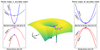Fig. 1. Curvature of the gravitational (Roche) potential near the inner and outer Lagrangian points around the donor star. The middle panel depicts an overall shape of the Roche potential in a binary in the corotating frame. The inner and outer Lagrangian points of the donor, indicated by a violet star and magenta cross, respectively, are where our computational domain is located. The $\stackrel{\sim }{x}$ axis of the domain is aligned with the binary axis and the z axis is parallel to the binary orbit axis. The left panels illustrate the significantly steeper curvature and shallower potential depth – both perpendicular (top) and parallel (bottom) to the binary axis – near the inner Lagrangian point than the outer Lagrangian point for a system where the donor and accretor have comparable masses (for instance, stellar binaries). The right panels show the same quantities for a case where the donor mass is significantly smaller than the accretor mass (for example, stellar extreme mass ratio inspiral). In this case, similar to the comparable mass ratio case, the potential near the outer Lagrangian point exhibits shallower curvature. However, the depths become comparable. In fact, the depths become equal as the ratio of the donor mass to the accretor mass approaches zero. The curvature of the potential near the Lagrangian points is primarily determined by the coefficients of the quadratic terms in the Taylor expansion of the Roche potential (Eq. (2)).

More specifically, for binaries with similar masses (for example, stellar binaries), the potential at the L_in point is much deeper and has a steeper curvature both parallel (larger |A|) and perpendicular (larger B and C) to the binary axis than at the L_out point. This implies that the donor star must significantly overfill RL for L_out overflow to occur. For example, for equal-mass binaries, L_out overflow can occur when the size of the donor is larger than that of RL by ≃30% (or relative overfilling factor ≳0.3). On the other hand, for binaries with very different mass ratios (for instance, stellar extreme mass ratio inspirals), the depths of the potential at the L_in and L_out points become comparable, although the potential at the L_in point remains lower. This means L_out outflow can begin even when the donor slightly overfills the RL (for instance, relative overfilling factor ≳10⁻³ for stellar extreme mass ratio inspiral with mass ratio of 10⁻⁶). However, the curvature of the potential near the L_out point is shallower, allowing for a larger cross-section of overflowing streams. This indicates that the L_out overflow rate can be comparable to or potentially larger than the L_in rate when the donor star overfills its RL sufficiently.

3. Summary of assumptions and numerical methods

In this section, we provide a summary of key assumptions and numerical methods to perform 3D hydrodynamic simulations of mass transfer near the L point, incorporating the approximate Roche potential – red quadratic in position (Eq. (2)) – and the Coriolis force in the corotating frame. We refer to Appendices A and B for more details.

We used the finite-volume adaptive mesh refinement magnetohydrodynamics code ATHENA++ (Stone et al. 2008, 2020). Our Cartesian computational domain focuses on the region near each of the L_in and L_out points around the donor (see Fig. B.1 for a schematic diagram of the location and shape of the domain) The x axis is aligned with the binary axis and the z axis parallel to the orbit axis, with the coordinate center in the domain coinciding with the Lagrangian point.

A key advantage of our methods is its scalability. We introduced scaling factors, including the RL overfilling factor, to make the hydrodynamics equations with the Roche potential and initial conditions dimensionless (see Appendix A.4 for the complete list of scaling factors). In particular, the quadratic form of the potential allows defining a natural length scale for the problem as the square root of the potential difference. This means the problem retains the same dimensionless shape regardless of the exact value of the potential difference. In cases where the stellar surface is approximated to have a finite size (see the “adiabatic” case below), the potential difference corresponds to the overfilling factor, and the scalability enables generalizing simulation results for a given mass-transferring system to arbitrarily small overfilling factors. However, the accuracy of our results, when converted from code units to physical units, is influenced by the overfilling factor. Specifically, scaling to smaller overfilling factors yields more accurate results for a given computational box size, as the approximated potential deviates more significantly from the exact potential at larger overfilling factors (see also Fig. A.2). Therefore, our approach is best suited for modeling the onset of mass transfer with small relative overfilling factors (≲10⁻³ − 10⁻²).

By focusing on overflow near the Lagrangian point with adaptive mesh refinement, we achieved unprecedented resolution: 20 − 80 cells across the width of the stream crossing the Lagrangian point and 10 − 50 cells per pressure scale height within the donor. This level of resolution for the overflow stream was achieved in previous simulations with relative overfilling factors greater than 0.01 (e.g., Dickson 2024). However, the scalability of our method ensures that this high resolution is maintained even for arbitrarily small overfilling factors. In addition, to our knowledge, no previous simulations have achieved such a high resolution for both the donor’s surface and the overflowing stream. We confirmed through resolution tests that the resolution is sufficiently high to produce converged results (see Appendix B.1).

We made two key assumptions: (1) the donor’s surface before the onset of mass transfer is in hydrostatic equilibrium and follows a polytropic relation (P ∝ ρ^γ with a constant polytropic exponent γ, where P is the pressure and ρ is the density), and (2) the gas behaves as an ideal gas. While simplified, these assumptions are necessary for scalability and allow for fully analytical solutions for steady-state overflow (see Appendix A.3) following Ritter (1988) and Kolb & Ritter (1990). Their analytic models have been widely used in stellar evolution codes such as MESA, but they account only for mass transfer through the L_in point. In this work, we extended their models to include mass transfer through the L_out point. By directly comparing analytic predictions with our simulation results for both the L_in and L_out points, we can achieve a critical assessment of the assumptions underlying analytic solutions, refine the mass transfer prescriptions for the L_in point, and provide prescriptions for the L_out point that can be readily implemented in stellar evolution codes.

Under these assumptions, we first constructed an analytic solution for overcontact binaries in hydrostatic equilibrium (see Appendix A.2) and mapped it onto our numerical domain as the initial condition. We then applied an outflow boundary condition along a boundary facing the accretor (see Fig. B.1). As a result, gas beyond the Lagrangian point – toward the outflow-imposed boundary (namely, toward the accretor) – quickly evacuates, while the donor on the opposite side begins transferring mass due to its initial RL overfilling.

We examine two cases:

• Adiabatic: The initial structure follows a polytropic relation with γ = 5/3, which evolves using an equation of state P = (Γ − 1)u with Γ = 5/3. Here, u is the internal energy density. Because of the same values of γ (for the initial structure) and Γ (for hydrodynamic evolution) and the absence of shocks, the entropy remains constant throughout the domain. This represents optically thick overflowing streams, such as the case with convective envelopes where the photosphere is outside the RL.

• Isothermal: The initial structure follows a polytropic relation with γ = 1, which evolves assuming a constant P/ρ. This corresponds to the scenario where the transferring mass is optically thin (for example, photosphere inside the RL), maintaining the same sound speed.

For each case, we simulated a wide range of mass ratio: q = 10⁻⁶ − 10 for the inner L_in and outer L_out Lagrangian points around the donor. Here, the mass ratio q is defined as the donor-to-accretor mass ratio: For example, q > 1 corresponds to overflow from a more massive donor to less massive accretor, while q = 10⁻⁶ corresponds to overflow onto a very massive accretor like a supermassive black hole. To examine the effect of the Coriolis force, we also performed an additional simulation for q = 1 and L_in with γ = 5/3, excluding the Coriolis force. We provide the complete list of our models in Table B.1.

4. Results

In this section, we present results for stream morphology, which we compare with assumptions made in analytic models, and for mass transfer rates, which we compare with the corresponding analytic predictions, whose full derivations are provided in Appendix A. We provide results using dimensionless quantities scaled by characteristic scales of a given binary system, denoted by a tilde (for instance, $\stackrel{\sim }{t}$ and $\stackrel{\sim }{\rho }$). Conversion between scaled and physical units can be performed using the scaling factors given in Appendix A.4.

Turning on the outflow boundary condition leads to the sudden onset of a gas flow beyond the Lagrangian point. Due to the sudden change in state, the donor’s surface and overflowing stream briefly undergo a transient phase. However, they soon reach a steady state, meaning no significant temporal evolution of gas morphology and the mass transfer rate. Therefore, we only focus on the morphology of streams and the mass overflow rate which have reached a steady state. For straightforward application of our results in stellar evolution and population synthesis codes, we provide fitting formulas for some of the main quantities using the identical mathematical form : a + btanh[clog₁₀(q)+d]^e.

4.1. Stream morphology

4.1.1. Origin of the main stream

In all our models including both adiabatic and isothermal cases, the main streams originate from the “trailing” side of the donor star along its orbital path because of the Coriolis force. We illustrate the origin of the main stream in Fig. 2 using the trajectories of tracer particles around L_in for q = 1 in the midplane. The particles are initially distributed in a region of the donor with ${10}^{-3}\lesssim \stackrel{\sim }{\rho }\lesssim 20$, with their distribution scaling with the initial $\stackrel{\sim }{\rho }$. This ensures complete coverage of the region near the Lagrangian point and along the RL boundaries. Their trajectories are integrated for $\stackrel{\sim }{t}\simeq 20$, after the system reached a steady state, under the assumption that the particles advect with the gas. It is worth noting that the deepest initial locations of the particles that have been transferred to the accretor largely depend on the integration duration. Consequently, this figure is intended to illustrate the overall shape of the main streams, rather than the maximum depth within the donor from which the gas can flow over the Lagrangian point. In the adiabatic case without the Coriolis force (left), the main stream originates from the middle. In contrast, in the same case with the Coriolis force (middle), the Coriolis force breaks the symmetry around the axis connecting the binary components (or “binary axis” at $\stackrel{\sim }{\mathit{y}}=0$), resulting in the main overflowing stream originating from the trailing side of the donor, and then being bent beyond the Lagrangian point toward the trailing side of the accretor. Similar features are found in the isothermal case with q = 1 (right), and, indeed, in all our models. This main stream morphology resembles the stream motion near the Lagrangian point analytically predicted by Lubow & Shu (1975) (see their Fig. 3) and the streams observed in hydrodynamics simulations of the L_in streams for an equal-mass semidetached binary by Oka et al. (2002).

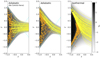Fig. 2. Trajectories of particles for a steady state solution of an equal-mass adiabatic case (left: without Coriolis force and middle: with Coriolis force) and an equal-mass isothermal case (right) in the midplane around the inner Lagrangian point, plotted over the density distribution. The particles are initially distributed following the same distribution of the initial density profile over a region with ${10}^{-3}\lesssim \stackrel{\sim }{\rho }\lesssim 20$ and their trajectories are integrated for $\stackrel{\sim }{t}\simeq 20$ since the flow reaches a steady state, assuming the particles are advected with the gas. Crosses at one end of the lines indicate the initial locations of the particles. We distinguish particles that reach beyond the Lagrangian point (yellow) from those that remain inside the donor (orange) over the integration duration.

4.1.2. Sonic surface

The sonic surface – the surface where the Mach number equals to unity – is expected to be located in a very small neighborhood of the Lagrangian point (for example, on the scale of c_s/Ω, where c_s is the sound speed at the surface of the donor; Lubow & Shu 1975). Analytic models (e.g., Ritter 1988; Kolb & Ritter 1990; Ge et al. 2010; Jackson et al. 2017; Cehula & Pejcha 2023) or semi-analytic model (e.g., Pavlovskii & Ivanova 2015) typically estimate the mass transfer rate by assuming that the sonic speed is a flat surface perpendicular to the binary axis, intersecting the Lagrangian point. Therefore, the relative position of the sonic surface provides insight into how the assumptions about fluid properties in analytic models – and, consequently, the mass flow rate – differ from our numerical solutions.

We find that the sonic surface is not normal to the binary axis. In the adiabatic case, it is concave both vertically and laterally. Because of the Coriolis force, the sonic surface becomes asymmetric, stretching further toward the trailing side of the accretor, in the mid-plane, while remaining axisymmetric along the vertical direction. In the isothermal case, on the other hand, the sonic surface is vertically flat, but similar to the adiabatic case, it is laterally concave. This behavior is illustrated in Fig. 3. The asymmetric, concave shape means that the fluid velocity along the plane normal to the binary axis is not the sonic speed, contrary to the assumption commonly made in analytic models. Even the sonic surface does not always intersect the Lagrangian point in both cases – Mach number at the Lagrangian point 0.9 − 1 for the adiabatic case and 1.1–1.3 for the isothermal case. This asymmetric shape of the sonic surface is also found in 3D hydrodynamics simulations of mass transfer in semi-detached binaries by Oka et al. (2002) (see their Fig. 7) and Dickson (2024) (see their Fig. 5).

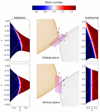Fig. 3. Shape and location of the sonic surface near the inner Lagrangian point. The 3D images of the binary near the Lagrangian point in the center show the orientation of the 2D plane in which the 2D distribution of Mach number is depicted – mid- (top) and vertical (bottom) slices. The panels on the left show the distributions for the equal-mass adiabatic case, while those on the right correspond to the equal-mass isothermal case. In the panels showing the Mach number distribution, the dashed diagonal orange lines depict the shape of the Roche lobe.

4.1.3. Vertical and lateral motion of overflowing streams

In analytic studies of isothermal mass transfer, it is often assumed that the overflowing stream at the inner Lagrangian point remains close to hydrostatic equilibrium along the vertical direction (Lubow & Shu 1975) or along both vertical and lateral directions (Meyer & Meyer-Hofmeister 1983; Ritter 1988; Cehula & Pejcha 2023), allowing an analytic expression for the fluid density near the Lagrangian point. Furthermore, Lubow & Shu (1975) suggested the possibility of lateral expansion in the overflowing stream (see their Fig. 3). In fact, we find that, in isothermal cases, the overflowing gas exhibits no significant vertical motion but does show lateral expansion, as assumed by Lubow & Shu (1975). The expansion speed of most overflowing gas reaches up to a few tens of % of the overflowing speed toward the donor (or ${\stackrel{\sim }{v}}^v/{\stackrel{\sim }{v}}^x\lesssim 0.2-0.3$). While the negligible vertical motion suggests that the gas is in hydrostatic equilibrium normal to the binary plane, the lateral expansion motion implies that the gas is not necessarily in hydrostatic equilibrium within the binary plane. This behavior is demonstrated in the top panels of Fig. 4 for the equal-mass, L_in mass transfer. On the other hand, in adiabatic cases, the main stream exhibits overall compressional motion toward the Lagrangian point, with speeds up to a few tens of % of the overflowing speed toward the donor, which is illustrated in the bottom panels of Fig. 4. The vertical and lateral motions in both cases can be understood qualitatively by considering how gas pressure responds to changes in density. As the gas overflows through the L point, acceleration toward the accretor causes the overflowing stream density to decrease. In the isothermal case, because the temperature remains constant – and thus the pressure decreases only linearly with density (P ∝ ρ) – the pressure can remain significant enough for the gas to expand or remain in hydrostatic equilibrium. In contrast, in the adiabatic case, the pressure drops more steeply (P ∝ ρ^5/3), so the stream tends to contract due to the reduced thermal pressure. These trends are consistent across all models.

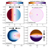Fig. 4. Vertical and lateral motion of overflowing stream, relative to the motion toward the accretor, in the plane normal to the binary axis and intersecting the Lagrangian point (magenta cross), with the Coriolis force. Gas with $\stackrel{\sim }{\rho }<{10}^{-3}$ (white background), which contributes negligibly to the overflowing stream, is masked out for better visualization. ${\stackrel{\sim }{v}}^i$ (i = x, y, z) is the ith velocity component relative to the Lagrangian point. In both cases – adiabatic (left) and isothermal (right), we assume an equal-mass binary. The hatched areas indicate the velocity ratios less than 0.05, suggesting that the gas may be assumed to be in hydrostatic equilibrium. The arrows show the overall motion of the stream.

4.1.4. Tilt angle of overflowing gas

The Coriolis force bends the overflowing gas toward the trailing side of the accretor (see Fig. 2). The tilt angle θ of the overflowing stream relative to the binary axis, defined as $tan\theta =⟨{\stackrel{\sim }{v}}^{\mathit{y}}⟩/⟨{\stackrel{\sim }{v}}^x⟩$, is shown in Fig. 5 for the adiabatic (left) and isothermal (right) cases. Here, $⟨{\stackrel{\sim }{v}}^x⟩$ and $⟨{\stackrel{\sim }{v}}^{\mathit{y}}⟩$ is a mass-weighted average of ${\stackrel{\sim }{v}}^x$ ${\stackrel{\sim }{v}}^{\mathit{y}}$, respectively, across the right x− boundary. For L_in, θ varies within a relatively small range, peaking at q = 1 and ranging from −28° to −20° in the adiabatic case and −40° to −20° for the isothermal case. On the other hand, for L_out, θ decreases as q increases, ranging from −28° ( − 36° ) for q = 10⁻⁶ to −72° ( − 73° ) for q = 10 in the adiabatic (isothermal) case.

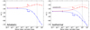Fig. 5. Angle of the transferring stream relative to the binary axis for adiabatic (left) and isothermal cases (right) in the presence of the Coriolis force. The angle is defined as $tan\theta =⟨{\stackrel{\sim }{v}}^{\mathit{y}}⟩/⟨{\stackrel{\sim }{v}}^x⟩$, where $⟨{\stackrel{\sim }{v}}^x⟩$ and $⟨{\stackrel{\sim }{v}}^{\mathit{y}}⟩$ are mass-weighted averages of ${\stackrel{\sim }{v}}^x$ and ${\stackrel{\sim }{v}}^{\mathit{y}}$ measured at the right x-boundary. The solid curves following the dots indicate the fitting formulae given in Eq. (3). The vertical solid gray lines indicate equal-mass binary. In the right panel, the dotted curves indicates the predictions of the tilt angle for the isothermal case by Lubow & Shu (1975).

This overall trend qualitatively follows the dependence of the RL intersection angle at the Lagrangian point relative to the binary axis, given by ${\theta }_{\mathrm{RL}}={tan}^{-1}(\sqrt{A/B})$. Here, A and B are the coefficients of the quadratic terms in $\stackrel{\sim }{x}$ and $\stackrel{\sim }{\mathit{y}}$, respectively, for the approximated Roche potential given in Eq. (2). However, θ_RL does not fully account for the trend quantitatively. The overall range of θ/θ_RL ranges from 0.6 − 0.3 for L_in and 0.5 − 1 for L_out. In fact, Lubow & Shu (1975) estimated θ for the isothermal case using a perturbation analysis of the conservation equation for mass and momentum near the Lagrangian point, assuming vertical hydrostatic equilibrium. Their expression, $cos2\theta =-4/3C+\sqrt{1-8/9C}$ (their Equation (24), dotted lines in Fig. 5), consistently underestimates θ compared to our numerical estimates by ≲20 − 30% for all isothermal models¹.

We provide the fitting formula for θ in degrees with errors ≲4%,

$$\begin{array}{c}\hfill \theta =a+b{[tanh(c{log}_{10}(q)+d)]}^e,\end{array}$$(3)

where for mass flow over the L_in point (e = 2),

$$\begin{array}{cc}& a=-19.1,b=-8.92,c=0.541,d=0\text{Adiabatic case},\hfill \\ \hfill & a=-25.0,b=-11.2,c=0.558,d=0\text{Isothermal case},\hfill \end{array}$$

and for mass flow over the L_out point (e = 1),

$$\begin{array}{cc}& a=-57.6,b=-28.6,c=0.697,d=-0.202\text{Adiabatic case},\hfill \\ \hfill & a=-62.9,b=-26.3,c=0.525,d=-0.176\text{Isothermal case}.\hfill \end{array}$$

4.2. Mass transfer rate

In Figure 6, we compare the mass transfer rate from our simulations to the analytic solution for the adiabatic (Eq. (A.25)) and isothermal cases (Eq. (A.30)). We estimate the mass transfer rate as $\dot{\stackrel{\sim }{M}}={\displaystyle \int \int \stackrel{\sim }{\rho }}{\stackrel{\sim }{v}}^x\mathrm{d}\stackrel{\sim }{\mathit{y}}\mathrm{d}\stackrel{\sim }{z}$ at the right x-boundary. We find that the numerically computed mass transfer rates, which include the effects of the Coriolis force, are lower than the analytic estimates by 50 − 70% for L_in and by up to 10 − 50% for L_out across a wide range of q, from 10⁻⁶ to 10. Notably, for the L_in, equal-mass (q = 1) adiabatic case, when the Coriolis force is excluded, the numerically estimated rate is only 4% smaller than the analytic estimate. This suggests that the discrepancy between the numerical and analytic results is caused by the Coriolis force.

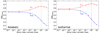Fig. 6. Ratio of the numerically estimated mass transfer rate $\dot{\stackrel{\sim }{M}}$ in the presence of the Coriolis force to the analytic estimates ${\dot{\stackrel{\sim }{M}}}_{\mathrm{analytic}}$ (Eq. (A.25) for for the adiabatic case (left) and Eq. (A.30) for the isothermal case (right)). The solid curves following the dots indicate the fitting formulae given in Eq. (A.2). The solid vertical gray lines indicate equal-mass binary. Note that no assumption for the overfilling factor is made for this comparison as the overfilling factor is a scaling factor (see Eqs. (A.25) and (A.30)). We refer to Fig. 9 for a comparison of $\dot{\stackrel{\sim }{M}}$ between Lin and Lout for a given overfilling factor.

To understand the main cause of the discrepancy, we compare numerical solutions to analytic solutions for $\stackrel{\sim }{\rho }$, ${\stackrel{\sim }{v}}^x$, and $\stackrel{\sim }{\rho }{\stackrel{\sim }{v}}^x$ along the $\stackrel{\sim }{\mathit{y}}$ axis intersecting the L_in point ($\stackrel{\sim }{x}=0$) in the equal-mass cases separately to their analytic solutions in Fig. 7. Let us first examine the adiabatic cases without (left column) and with (middle column) the Coriolis force. Without the Coriolis force, the density profile is symmetric around $\stackrel{\sim }{\mathit{y}}=0$, as expected, but is generally larger than its analytic solution. Conversely, ${\stackrel{\sim }{v}}^x$ is smaller than its analytic solution by a similar amount. The higher $\stackrel{\sim }{\rho }$ and smaller ${\stackrel{\sim }{v}}^x$ almost perfectly cancel each other, resulting in $\stackrel{\sim }{\rho }{\stackrel{\sim }{v}}^x$ values that closely match the analytic solution.

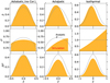Fig. 7. Comparison between numerical (orange) and analytic solutions (gray lines). We compare density $\stackrel{\sim }{\rho }$ (top row), velocity toward the accretor ${\stackrel{\sim }{v}}^x$ (middle row), and $\stackrel{\sim }{\rho }{\stackrel{\sim }{v}}^x$ (bottom row) from our simulations along the $\stackrel{\sim }{\mathit{y}}$ axis intersecting the inner Lagrangian point ($\stackrel{\sim }{\mathit{y}}=0$) to the corresponding analytic solutions. We consider equal-mass binaries for both adiabatic – without (left column) and with (middle column) the Coriolis force – and isothermal cases with the Coriolis force (right column).

When the Coriolis force is introduced (middle column of Fig. 7), the density profile shifts to negative $\stackrel{\sim }{\mathit{y}}$, while the stream boundary at $\stackrel{\sim }{\mathit{y}}=-0.5$ remains unchanged. This means that the stream is compressed – the density peak is 1.1 times larger than that of the analytic solution – and the overall stream width decreases, with the full width at half maximum being 1.2 times smaller than that of the analytic profile. Meanwhile, ${\stackrel{\sim }{v}}^x$ becomes asymmetric around $\stackrel{\sim }{\mathit{y}}=0$, increasing monotonically with $\stackrel{\sim }{\mathit{y}}$ within the stream and reaching slightly above 0.6. Consequently, ${\stackrel{\sim }{v}}^x$ is smaller than its analytic solution across more than 80% of the stream’s width. At the density peak ($\stackrel{\sim }{\mathit{y}}\simeq -0.1$), ${\stackrel{\sim }{v}}^x$ is smaller than its analytic solution by a factor of 1.5. Interestingly, despite the asymmetry in $\stackrel{\sim }{\rho }$ and ${\stackrel{\sim }{v}}^x$, their product, $\stackrel{\sim }{\rho }{\stackrel{\sim }{v}}^x$, exhibits a more symmetric profile, extending only slightly further toward negative $\stackrel{\sim }{\mathit{y}}$. Overall, $\stackrel{\sim }{\rho }{\stackrel{\sim }{v}}^x$ remains consistently smaller than its analytic counterpart. This suppression is primarily driven by the reduction in ${\stackrel{\sim }{v}}^x$ and effective stream cross section, evidenced by three key factors: 1) $\stackrel{\sim }{\rho }{\stackrel{\sim }{v}}^x$ remains suppressed despite the increase in $\stackrel{\sim }{\rho }$ for $\stackrel{\sim }{\mathit{y}}<0$, 2) on the opposite side, the suppression of $\stackrel{\sim }{\rho }$ only partially contributes to the reduction in $\stackrel{\sim }{\rho }{\stackrel{\sim }{v}}^x$, and 3) the asymmetry in $\stackrel{\sim }{\rho }$ and ${\stackrel{\sim }{v}}^x$ in the opposite sense effectively reduces the width of the stream.

The density profile in the isothermal case, shown in the right column of Figure 7, is also shifted toward negative $\stackrel{\sim }{\mathit{y}}$ because of the Coriolis force, with its density peak lower than that of the analytic counterpart. For $\stackrel{\sim }{y}$ values smaller than the peak location, $\stackrel{\sim }{\rho }$ remains slightly above the analytic profile while, on the opposite side, $\stackrel{\sim }{\rho }$ is consistently lower. This suggests the stream is not compressed, but rather becomes less dense with a smaller width. The velocity profile is a monotonically increasing function of $\stackrel{\sim }{\mathit{y}}$ within the stream width ($-1\lesssim \stackrel{\sim }{\mathit{y}}\lesssim 1$). Similarly to the adiabatic case with the Coriolis force, despite the asymmetric shapes of $\stackrel{\sim }{\rho }$ and ${\stackrel{\sim }{v}}^x$, the product $\stackrel{\sim }{\rho }{\stackrel{\sim }{v}}^x$ remains symmetric around $\stackrel{\sim }{y}=0$ and is consistently smaller than its analytic counterpart. However, unlike the adiabatic case, it is difficult to determine which component primarily contributes to the suppression of $\dot{\stackrel{\sim }{M}}$ relative to ${\dot{\stackrel{\sim }{M}}}_{\mathrm{analytic}}$. The reduction in ${\stackrel{\sim }{v}}^x$ is the dominant factor for $\stackrel{\sim }{\mathit{y}}<0$, whereas for $\stackrel{\sim }{\mathit{y}}>0$, the suppression of $\stackrel{\sim }{\rho }$ plays a larger role.

The fact that the Coriolis force results in the suppression of $\dot{\stackrel{\sim }{M}}$ may suggest a possible correlation of the $\dot{\stackrel{\sim }{M}}$ suppression with the overflow tilt angle (θ), the RL intersection angle (θ_RL), or possibly both. The qualitative similarity in the dependence of these quantities on the mass ratio further strengthens the possibility of their connection. This is understandable, considering the Coriolis force essentially results in the main stream coming in parallel to the RL potential (so θ_RL) inside the donor before crossing the Lagrangian point. And beyond the Lagrangian point, the overflowing gas speed determines the strength of the Coriolis force exerted on it, tilting the overflowing stream and creating the non $\stackrel{\sim }{y}$-component of velocity (so θ).

It turns out that the correction by θ_RL, namely cos θ_RL, reduces the discrepancy between the numerically and analytically estimated rates significantly more than the correction by θ. Overall, the cos θ_RL correction (or $cos\theta \dot{\stackrel{\sim }{M}}/{\dot{\stackrel{\sim }{M}}}_{\mathrm{analytic}}$) leads to smaller deviations from analytic solutions within up to a factor of 1.3 for L_in and 2 for L_out in both the adiabatic and isothermal cases. When corrected with cos θ, the overall deviations from analytic solutions remain nearly the same as those without the correction because cos θ is generally too small to make significant corrections. While the difference in the level of correction between the two angles is substantial, it is not entirely clear why θ_RL serves as a better correction factor.

Finally, we provide the fitting formula for $\dot{\stackrel{\sim }{M}}/{\dot{\stackrel{\sim }{M}}}_{\mathrm{analytic}}$ with errors ≲4%, sharing the identical functional form of the fitting formula for θ given in Eq. (3),

$$\begin{array}{c}\hfill \frac{\dot{\stackrel{\sim }{M}}}{{\dot{\stackrel{\sim }{M}}}_{\mathrm{analytic}}}=a+b{[tanh(c{log}_{10}(q)+d)]}^e,\end{array}$$(4)

where for mass flow over the L_in point (e = 2),

$$\begin{array}{cc}& a=0.649,b=-0.151,c=0.540,d=-0.037\text{Adiabatic case},\hfill \\ \hfill & a=0.721,b=-0.149,c=0.522,d=0,\text{Isothermal case},\hfill \end{array}$$

and for mass flow over the L_out point (e = 1),

$$\begin{array}{cc}& a=0.243,b=-0.243,c=-0.658,d=0\text{Adiabatic case},\hfill \\ \hfill & a=0.280,b=0.280,c=-0.650,d=0\text{Isothermal case}.\hfill \end{array}$$

5. Proposed improvement for implementation in binary evolution codes

In this section, we extend the analytic models by Ritter (1988) and Kolb & Ritter (1990) to account for both the L_in and L_out points valid over a wide range of mass ratios. We provide a fitting formula (Eq. (8)) below that can be readily implemented in stellar evolution codes such as MESA where their original models are already in use. Outflow through L_out was considered by Marchant et al. (2021), who accounted for the proper geometry of the Roche potential near L_out based on the models of Ritter (1988) and Kolb & Ritter (1990) (see also Misra et al. 2020). However, we attempt to further incorporate the effects of hydrodynamics and the Coriolis force into their models.

Ritter (1988) and Kolb & Ritter (1990) developed analytic models for the L_in point with isothermal and adiabatic gas, respectively, assuming steady flow of overflowing gas. In both cases, the mass overflow rate through the L_in point is given by

$$\begin{array}{c}\hfill \dot{M}={\displaystyle {\int }_{\mathrm{L}}}{\rho }_{\mathrm{L}}{v}_{\mathrm{L}}\mathrm{d}A,\end{array}$$(5)

where ρ_L and v_L are density and speed at the Lagrangian point. The mass flux ρ_Lv_L is integrated over the surface (the “sonic” surface) normal to the binary axis and intersecting the Lagrangian point, where the flow speed is assumed to equal the sound speed. The assumption of steady-state flow implies a constant Bernoulli constant (see Appendix A), which analytically connects the density and sound speed at the photosphere, assumed to be in hydrostatic equilibrium, to those at the sonic surface.

In both the isothermal and adiabatic cases, the resulting integration contains the geometric term F₁(q), following the notation of Kolb & Ritter (1990)², which accounts for the cross-section of the overflowing stream (Eq. (A2) for the isothermal case and A17 for the adiabatic case in Kolb & Ritter 1990). F₁(q) depends on the effective size of RL and two coefficients of the quadratic terms in the Taylor expansion of the Roche potential. Specifically, F₁(q) and two quadratic coefficients (B and C in Eq. (1)) are related by

$$\begin{array}{c}\hfill F_1(q)=\frac{q}{1+q}\frac{f_1^{-3}}{\sqrt{\mathit{BC}}},\end{array}$$(6)

where f₁ is the effective size of RL in units of the semimajor axis. Because no analytic expression for F₁ exists, Ritter (1988) provided a fitting formula (their Eq. (A9)), valid for the inner Lagrangian point with mass ratios 0.1 ≤ q ≤ 2. In Fig. 8, we depict the fitting formula (dashed gray line), which reproduces the numerically estimated F₁ (solid gray line) within 40% over the stated range of mass ratios. This fitting formula is used in the functions get_info_for_ritter(), calculate_kolb_mdot_thick() to calculate the overflow rate in MESA [version r24.08.1].

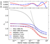Fig. 8. Dynamical term ℱ1 accounting for the stream cross-section, hydrodynamical effects and the Coriolis force (colored lines) in the calculation of the mass transfer rate. In the bottom panel, the solid gray line represents the term only accounting for the potential geometry for the inner Lagrangian point introduced in Ritter (1988), who also provided a fitting formula (dashed gray line). The thick colored lines show the improved dynamical term for the adiabatic (dot-dashed lines) and isothermal (dashed lines) cases and the Roche potential geometry for the inner (red) and outer (blue) Lagrangian points. The fitting formula (thinner solid lines), closely overlapping with the thicker lines, reproduces the factors within 2.5% across the full range of mass ratio considered.

The easiest way to incorporate the correction factor for Ṁ discussed in Sect. 4.2 may be to include it directly in F₁, using the ratio $\dot{\stackrel{\sim }{M}}/{\dot{\stackrel{\sim }{M}}}_{\mathrm{analytic}}$ from Eq. (A.2), so that

$$\begin{array}{c}\hfill {\mathcal{F}}_1(q)=\frac{q}{1+q}\frac{f_1^{-3}}{\sqrt{\mathit{BC}}}\frac{\dot{\stackrel{\sim }{M}}}{{\dot{\stackrel{\sim }{M}}}_{\mathrm{analytic}}}.\end{array}$$(7)

This new “dynamical” factor accounts not only for the different geometry of the L_in and L_out points (using B and C for each point), but also for the hydrodynamical effects and the Coriolis force, which is shown in Fig. 8 as red (L_in point) and blue (L_out point) lines. We estimated f₁ for the equipotential of the L_in point using Eq. (14) in Jackson et al. (2017) and for that of the L_out point using Eq. (3) in Marchant et al. (2021).

To further facilitate implementation, we also provide a fitting formula for ℱ₁ that only depends on the mass ratio, with an error ≲2.5% in the range of 10⁻⁶ ≤ q ≤ 10³. The mathematical form of the fitting formula is the same for all four cases, and consistent with the form used in all previously provided fitting expressions:

$$\begin{array}{c}\hfill {\mathcal{F}}_1(q)=a+btanh[c{log}_{10}(q)+d],\end{array}$$(8)

where for mass flow over the L_in point,

$$\begin{array}{cc}& a=0.720,b=0.473,c=-0.676,d=0.150\text{Adiabatic case},\hfill \\ \hfill & a=0.827,b=0.546,c=-0.659,d=0.095\text{Isothermal case},\hfill \end{array}$$

and for mass flow over the L_out point,

$$\begin{array}{cc}& a=0.889,b=0.307,c=-0.786,d=0.551\text{Adiabatic case},\hfill \\ \hfill & a=1.037,b=0.337,c=-0.778,d=0.512\text{Isothermal case}.\hfill \end{array}$$

This implementation leads to three key advantages: (1) ℱ₁(q) applies over a wider range of mass ratios; (2) ℱ₁(q) accounts for hydrodynamical effects, Coriolis force, and the Roche potential geometry of both the L_in and L_out points in adiabatic and isothermal cases; and (3) in practice, implementing ℱ₁(q) requires minimal revision to existing codes where F₁ is already in use. One only needs to replace the original expression (Eq. (6)) with the expression for ℱ₁ (Eq. (8))³.

However, there are also some caveats to the extended prescriptions: (1) they are based on two simplified assumptions – a polytopic relation for the donor’s envelope and an ideal-gas equation of state. (2) Our approximation for the Roche potential becomes less accurate at larger overfilling factors. Although we cannot precisely determine the extent of the resulting error in the hydrodynamical evolution of overflowing streams and the overflowing rate, based on the relative errors in the potential values, caution is advised when applying our prescriptions to systems with overfilling factors greater than 10⁻³ − 10⁻². We plan to refine these prescriptions in a follow-up study using simulations that incorporate the full expression of the Roche potential and account for realistic stellar structure.

Using these new prescriptions, we compare the L_out mass transfer rate to that for L_in in Fig. 9, as a function of the relative overfilling factor, assuming adiabatic gas⁴. We also compare them to the ratios without our correction factor (dashed lines). The range of the relative overfilling factor considered in the plot is already worryingly high for our prescriptions to remain valid. However, we show this figure to demonstrate what our prescriptions can calculate. The characteristic overfilling factors for the onset of overflow through the L_out point are smaller for smaller mass ratios, as the potential depths at the L_in and L_out points become comparable (see Fig. 1)⁵. Once L_out overflow begins, its rate increases more rapidly with overfilling than the L_in rate, leading to a rising trend with the overfilling factor. For q = 10⁻⁶, the L_out rate becomes comparable to the L_in rate at overfilling factors above 0.1 and our correction factor does not make a significant difference. We note that the rate ratio exceeds unity when q ≲ 10⁻⁸, indicating the L_out outflow would dominate over the L_in mass transfer. For binaries with comparable masses, while the L_out overflow remains subdominant even at the overfilling factor of order unity, our correction factor can lead to a significant suppression of the L_out overflow relative to the L_in outflow. For example, for a mass ratio of 10, Ṁ_out/Ṁ_in ≲ 0.1 with our correction factor, compared to Ṁ_out/Ṁ_in ≲ 0.4 without it.

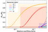Fig. 9. Onset of outflow through the outer Lagrangian point and the ratio of the mass transfer rate between the inner (Ṁin) and outer (Ṁout) Lagrangian points. The solid (dashed) lines represent the ratios predicted by the extension of Kolb & Ritter (1990) with (without) our correction factors. The star markers on the zero line indicate the characteristic relative overfilling factors at which outflow through the Lout point begins. The colored regions represent the range of overfilling factors for which outflow occurs through both Lagrangian points, as well as the maximum rate ratio over the range of parameters considered.

6. Discussion

6.1. Comparison to previous analytic work

We compared our simulation results with predictions from prior analytic models in Sect. 4. For clarity, we summarize the key comparisons here and in Table 1. The main assumptions of analytic models are:

1. Steady-state overflow: Most models (e.g., Paczyński & Sienkiewicz 1972; Lubow & Shu 1975; Ritter 1988; Kolb & Ritter 1990; Ge et al. 2010; Pavlovskii & Ivanova 2015; Jackson et al. 2017; Marchant et al. 2021) assume a steady-state overflow, enabling use of the Bernoulli theorem. Our simulations confirm this if the envelope lacks entropy stratification.

2. Origin of the main stream: Analytic models using the Bernoulli theorem (e.g., Paczyński & Sienkiewicz 1972; Ritter 1988; Kolb & Ritter 1990; Ge et al. 2010; Pavlovskii & Ivanova 2015; Jackson et al. 2017; Marchant et al. 2021) assume streams follow equipotentials from RL boundaries. An alternative view treats the L point as a de Laval nozzle, with streamlines freely crossing equipotentials (Cehula & Pejcha 2023). In this case, the main stream does not necessarily come from the sides, but rather from the middle along the binary axis. Our results resemble the nozzle picture without the Coriolis force, but with it, the stream originates mainly from the donor’s trailing side.

3. Sonic surface: The Bernoulli theorem, along with the fact that the inner L point is a saddle point, implies that the scale of the sound speed gradient should be comparable to the potential force gradient (Lubow & Shu 1975), leading to the conclusion that the fluid speed reaches the sonic speed at the L point. In fact, this assumption also leads to the maximum steady-state flow through the Lagrangian point (Paczyński & Sienkiewicz 1972). In later work (e.g., Meyer & Meyer-Hofmeister 1983; Ritter 1988; Kolb & Ritter 1990; Ge et al. 2010; Pavlovskii & Ivanova 2015; Jackson et al. 2017; Marchant et al. 2021), the overflow rate is estimated assuming the flow speed in the flat plane normal to the binary axis and intersecting the Lagrangian point is the same as the local sound speed. Our simulations show that the sonic surface is not flat, but rather asymmetrically concave, which does not necessarily intersect the Lagrangian point.

4. Hydrostatic equilibrium of the overflowing stream: It is often assumed that the overflowing isothermal stream near the Lagrangian point remains close to hydrostatic equilibrium normal to the binary axis – vertically (Lubow & Shu 1975) or both vertically and laterally (Meyer & Meyer-Hofmeister 1983; Ritter 1988; Ge et al. 2010; Jackson et al. 2017; Cehula & Pejcha 2023). This assumption allows for the analytical derivation of a fluid density profile near the Lagrangian point (for instance, an exponential profile), which determines the streams’ cross-section. We find that vertical (out-of-plane) hydrostatic balance holds, but in-plane equilibrium does not, which is consistent with Lubow & Shu (1975). While this does not entirely invalidate the use of a hydrostatic density structure – since the expansion speed reaches only up to tens of per cent of the overflowing speed – it suggests that one should use caution when making such an assumption.

5. Tilt angle of overflowing streams: The tilt angle of overflowing streams in the corotating frame is caused by the Coriolis force, which is often ignored in analytic models. Lubow & Shu (1975) estimated the title angle by investigating the asymptotic behavior of isothermal overflowing streams with the Coriolis force, which agrees with our simulation results to within 30%.

6.2. Dynamical mass transfer stability

Determining when mass transfer becomes unstable in binary evolution is critical to predicting the final outcomes of interacting binaries. One route to mass-transfer instability centers on how the donor star responds to mass loss during RL overflow, and whether the mass-transfer rate runs away to dynamical-timescale overflow. The canonical view was based on approximating the stellar structure with polytropes and assuming an adiabatic stellar response (e.g., Paczyński 1965; Hjellming & Webbink 1987). Those old adiabatic results remain widely used, despite the fact that calculations of mass transfer using detailed 1D stellar calculations find that thermal readjustment in the surface layers of the donor can help to significantly stabilize RL overflow (e.g., Podsiadlowski et al. 2002; Woods & Ivanova 2011; Temmink et al. 2023).

In the context of this work, the assumptions used in binary RL overflow calculations affect predictions for mass-transfer stability. Pavlovskii & Ivanova (2015), Marchant et al. (2021), and Cehula & Pejcha (2023) all adopted their respective updated schemes for treating Roche-lobe overflow and considered when the donor star became so large as to overflow L_out, carrying away additional orbital angular momentum and potentially leading to unstable mass transfer (e.g. Nariai & Sugimoto 1976; for other potential consequences of L_out overflow see also, for instance, Hubová & Pejcha 2019). The Pavlovskii & Ivanova (2015) scheme tends to stabilize mass transfer, as investigated by Pavlovskii et al. (2017). Conversely, Cehula & Pejcha (2023) showed a massive-star example in which their mass-transfer scheme more easily led to L_out overflow than when using the schemes from Kolb & Ritter (1990) or Marchant et al. (2021). Given the above, the results from our simulations relative to analytic estimates may be substantial enough to change the properties of final binary outcomes on an individual level. However, it remains unclear how the reduced mass transfer and enhanced angular momentum loss via L_out impact the statistical properties of a binary population, which requires a detailed population study.

Our simulations indeed provide information on the instantaneous angular momentum carried by the transferred mass near L_out. However, this would not be directly translated into true angular momentum loss. It is because the angular momentum of the transferred gas will continuously change due to the time-dependent potential of the binary until its motion becomes bound to an effectively single object, that is, either one of the binary components or the binary as a whole. Therefore, additional calculations are required to track the gas motion in order to quantify the true angular momentum loss. We will investigate this in a follow-up project.

7. Conclusion and summary

We presented 3D hydrodynamical simulations of binary mass transfer in the corotating frame with the Coriolis force, spanning mass ratios from 10⁻⁶ to 10 and considering both adiabatic and isothermal gases. The donor envelope followed a polytropic relation. Focusing on the vicinity of the inner and outer Lagrangian points, we achieved high resolution – 10–50 cells per scale height at the stellar surface and 20–80 cells across the stream. Near the L point, we used a second-order expansion of the Roche potential, allowing us to scale the problem with key parameters like the overfilling factor, and generalize results to arbitrarily small overfilling.

Our main goals were (1) to study the stream’s morphology, tilt, and vertical/lateral structure, and (2) to estimate mass transfer rates and compare them with steady-state analytic models (e.g., Ritter 1988; Kolb & Ritter 1990). The Coriolis force, which analytic models have often ignored, plays a central role in shaping the stream morphology, as well as determining the mass transfer rate. Our results can be summarized as:

– Properties of transferring streams: Without the Coriolis force, streams overflow symmetrically around the binary axis; with it, the main stream shifts to the donor’s trailing side, creating an asymmetric morphology. Accordingly, the sonic surface becomes asymmetrically concave, stretching further toward the trailing side of the accretor and not always intersecting the Lagrangian point. Tilt angles of the overflowing isothermal streams beyond the Lagrangian point agree with analytic predictions within 30%. In adiabatic cases, gas compresses toward the Lagrangian point; in isothermal cases, the stream remains vertically hydrostatic but expands laterally. We compare these findings to analytic assumptions in Sect. 6.1.

– Mass transfer rate: Simulated mass transfer rates with the Coriolis force remains consistently smaller than analytic solutions for steady-state overflow through the inner Lagrangian point. However, the difference is remarkably small – only by up to a factor of two across seven orders of magnitude in mass ratio. We extended the Ritter (1988) and Kolb & Ritter (1990) models to include outer Lagrangian point overflow; these can be integrated into existing stellar evolution codes with minimal changes. Discrepancies for the outer Lagrangian point remain modest – within a factor of ten for the same range of mass ratios. These differences primarily arise due to the Coriolis force, which reduces the stream cross-section and speed. Without the Coriolis force, simulations and analytic models agree within 5%. The dependence of the rate on mass ratio aligns with the Roche-lobe intersection angle and stream tilt.

Our 3D simulations provided numerical evidence to assess the validity of assumptions and predictions made in analytic models. In addition, we presented fitting formulas for key variables to improve existing models for the mass transfer rate and its stability. Although the results from our simulations cannot directly address the long-term effects of the corrected mass transfer rate on binary evolution, the corrections may significantly enhance the reliability of mass transfer models, including stability criteria. We employed polytropic relations for the stellar structure primarily for analytic tractability and comparison with analytic solutions. However, this assumption, along with the use of a simple equation of state, does not fully capture the complexity of realistic stellar models. In future work, we will improve our models by incorporating more realistic conditions, such as realistic envelope structure, an equation of state that accounts for partial ionization, convective motion, radiative processes, and magnetic fields.

Acknowledgments

TR is grateful to Norbert Langer and Ondřej Pejcha for useful discussions. TR thanks Alejandro Vigna-Gómez and Jakub Klencki for useful comments on the manuscript. The authors thank the anonymous referee for their constructive feedback and suggestions. The authors acknowledge support from the German Israel Foundation for Scientific Research & Development Research Grant No. I-873-303.5-2024. RS is supported by an ISF, BSF/NSF and MOST grants, and a Humboldt Fellowship. This research was supported in part by grant NSF PHY-2309135 to the Kavli Institute for Theoretical Physics (KITP). The simulations presented in this paper were conducted using computational resources (and/or scientific computing services) at the Max-Planck Computing & Data Facility. The authors gratefully acknowledge the scientific support and HPC resources provided by the Erlangen National High Performance Computing Center (NHR@FAU) of the Friedrich-Alexander-Universität Erlangen-Nürnberg (FAU) under the NHR projects b166ea10 and b222dd10. NHR funding is provided by federal and Bavarian state authorities. NHR@FAU hardware is partially funded by the German Research Foundation (DFG) – 440719683. In addition, some of the simulations were performed on the national supercomputer Hawk at the High Performance Computing Center Stuttgart (HLRS) under the grant number 44232.

References

Appendix A: Analytic solution

In this section, we derive analytic solutions for the internal structure of overcontact binaries in hydrostatic equilibrium with the Roche potential and a steady state overflow rate, assuming a polytropic relation. In addition, we introduce scaling factors to non-dimensionalize the problem.

A.1. Approximate Roche potential

In Sect. 2, we introduced an approximate expression for the Roche potential ϕ (Eq. (2))

$$\begin{array}{c}\hfill \varphi (x,y,z)\simeq \frac{1}{2}{\mathrm{\Omega }}^2(A{x}^2+B{y}^2+C{z}^2).\end{array}$$(A.1)

Note that while a higher-order expansion of the potential can be used, as done in Marchant et al. (2021), we adopt the second-order expansion for scalability. The coefficients A, B, and C can be computed numerically. In fact, in our hydrodynamical simulations, we used numerically computed values of those constants, which is shown in Fig. A.1. Notice that those coefficients for L_in are symmetric around q = 1 (for example, A and B are the same for the mass ratios q and 1/q).

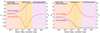Fig. A.1. Quadratic coefficients (Eq. (2)) that determine the curvature of the Roche potential near the Lagrangian point along the binary axis (A, left) and in the plane normal to the binary axis (B and C, right). The three coefficients are related by B = −(A + 3)/2 and C = B + 1. The red (blue) line represents the coefficients for the inner (outer) Lagrangian point, as a function of the donor mass over the accretor mass. In both panels, a few examples of mass transferring systems are presented in three different mass ratio regimes such as stellar extreme mass ratio inspiral (EMRI), even though the boundaries among these regimes are not clearly defined.

While a fitting formula for A was already provided in previous work (for instance, Eq. (10) in Jackson et al. 2017), we also provide a fitting formula for A sharing the same mathematical form of the fitting formulas for θ, $\dot{\stackrel{\sim }{M}}/{\dot{\stackrel{\sim }{M}}}_{\mathrm{analytic}}$, and ℱ₁, accurate within 6%

$$\begin{array}{c}\hfill A=a+btanh{[c{log}_{10}(q)+d]}^e,\end{array}$$(A.2)

where

$$\begin{array}{cc}& a=-16.8,b=7.53,c=0.67,d=0,e=2\text{for}{L}_{\mathrm{in}}\hfill \end{array}$$(A.3)

$$\begin{array}{cc}& a=-5.87,b=-2.87,c=-0.68,d=-0.67,e=1\text{for}{L}_{\mathrm{out}}.\hfill \end{array}$$(A.4)

Using Eq. (A.3), B = −(A + 3)/2 and C = −(A + 1)/2 can be estimated.

A.2. Hydrostatic equilibrium solutions in the Roche potential

We first derive hydrostatic equilibrium solutions for the internal structure of a contact binary in the Roche potential ϕ (Eq. (2)), assuming a polytropic relation P = Kρ^γ with a constant K and a constant γ. The hydrostatic equilibrium condition can be written as

$$\begin{array}{c}\hfill \mathrm{\Delta }\varphi +\gamma K{\rho }^{\gamma -2}\mathrm{\Delta }\rho =0.\end{array}$$(A.5)

Because the expression for ρ is different, depending on whether γ > 1 or γ = 1, we derive the expression for each case separately. Accordingly, based on the functional form of each solution, we introduce different scaling factors to non-dimensionlize both the equilibrium solution and ϕ. While the scaling factors are different, the expression for the scaled ϕ remains the same in both cases as

$$\begin{array}{c}\hfill \stackrel{\sim }{\varphi }(\stackrel{\sim }{x},\stackrel{\sim }{y},\stackrel{\sim }{z})=\frac{1}{2}(A{\stackrel{\sim }{x}}^2+B{\stackrel{\sim }{y}}^2+C{\stackrel{\sim }{z}}^2).\end{array}$$(A.6)

The tilde symbol, such as $\stackrel{\sim }{\varphi }$, indicates dimensionless quantities in this paper.

A.2.1. Adiabatic case with γ > 1

This case corresponds to overflowing streams that are optically thick (for instance, photosphere outside RL). Eq. (A.5) can be rewritten as

$$\begin{array}{c}\hfill \mathrm{\Delta }(\varphi +\frac{\gamma }{\gamma -1}K{\rho }^{\gamma -1})=0,\end{array}$$(A.7)

or

$$\begin{array}{c}\hfill \varphi +\frac{\gamma }{\gamma -1}K{\rho }^{\gamma -1}=\zeta ,\end{array}$$(A.8)

where ζ is a constant with the same dimension as ϕ. ζ corresponds to the potential at the surface of the donor (ϕ at ρ = 0), which is equivalent to the overfilling factor of the donor star. Using Eq. (2), and scaling the distance by ${\mathrm{\Omega }}^{-1}\sqrt{|\zeta |}$ and the density by (γK/(γ − 1)|ζ|)^{1/(γ − 1)}, we obtain the scaled expression for Eq. (A.8)

$$\begin{array}{c}\hfill \stackrel{\sim }{\varphi }+{\stackrel{\sim }{\rho }}^{\gamma -1}=\xi ,\end{array}$$(A.9)

where, ξ is either 1, corresponding to the overfilling case, or -1, corresponding to the underfilling case. Because we are interested in the overfilling case, we set ξ = 1 from now on. Using Eq. (A.6), we find the expression for $\stackrel{\sim }{\rho }$

$$\begin{array}{c}\hfill \stackrel{\sim }{\rho }={[1-\frac{A}{2}{\stackrel{\sim }{x}}^2-\frac{B}{2}{\stackrel{\sim }{y}}^2-\frac{C}{2}{\stackrel{\sim }{z}}^2]}^{\frac{1}{\gamma -1}}.\end{array}$$(A.10)

We have formulated the problem such that the potential at the surface of the overfilling donor (ξ), or equivalently the overfilling factor, acts as a scaling factor. As mentioned previously, this formulation allows us to scale our results to an arbitrarily small overfilling factor. However, the relationships between the overfilling factor and other scaling factors become less obvious in the scaled equations when interpreting our hydrodynamics simulation results in code units (see Sect. B). As an example, we illustrate how the relative overfilling factor α scales with the distance scaling factor for L_in in Fig. A.2. For a given α, we estimate ϕ at the donor surface relative to ϕ at the Lagrangian point using the higher-order expansion of the equipotential derived by Jackson et al. (2017). We also estimate R_d using the same expression for the potential. The distance scaling factor, in units of R_d, depends weakly on α, namely, ≃(0.6 − 1)×10⁻²(α/10⁻⁵)^0.5 for L_in within 10⁻⁶ ≲ q ≲ 10.

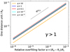Fig. A.2. Ratio of one distance code unit (${\mathrm{\Omega }}^{-1}\sqrt{|\xi |}$) to the effective size of the donor Rd, as a function of the relative overfilling factor α, defined as α = (Rd − RL)/RL. Here, RL is the effective RL size. We consider the inner Lagrangian point for this conversion.

A.2.2. Isothermal case with γ = 1

The isothermal case corresponds to the scenario where the transferring mass is optically thin (for instance, photosphere inside RL), maintaining the same sound speed. For this case, the equivalent form of Eq. (A.7) is

$$\begin{array}{c}\hfill \mathrm{\Delta }(\varphi +Kln\rho )=0,\end{array}$$(A.11)

which yields

$$\begin{array}{c}\hfill \rho ={\rho }_{0}exp(-\varphi /K).\end{array}$$(A.12)

Scaling the distance by $\sqrt{K}{\mathrm{\Omega }}^{-1}$ and the density by the arbitrary factor ρ₀, we obtain

$$\begin{array}{c}\hfill \stackrel{\sim }{\rho }=exp[-\frac{A}{2}{\stackrel{\sim }{x}}^2-\frac{B}{2}{\stackrel{\sim }{y}}^2-\frac{C}{2}{\stackrel{\sim }{z}}^2].\end{array}$$(A.13)

Because of the infinite extent of the envelope, such donors always overfill the RL.

A.3. Stationary solutions for mass overflow rate

In this section, we follow the assumptions made in Ritter (1988) for the isothermal case and Kolb & Ritter (1990) for the adiabatic case to derive the stationary solutions for the mass overflow rate. In the following derivation, we do not include the Coriolis force.

A.3.1. Adiabatic case with γ > 1

We start by considering the mass transfer rate exactly at the Lagrangian point. The corresponding 1D continuity equation integrates to

$$\begin{array}{c}\hfill \rho v={\dot{M}}_{\mathrm{L}}=\mathrm{constant}.\end{array}$$(A.14)

Notice that Ṁ_L in Eq. (A.14) has the same units as mass flux [mass / time / area ], not [mass / time]. However, for notational consistency, we continue to use the symbol Ṁ_L. Using Eq. (A.14) and assuming the polytropic relation, the momentum equation can be rewritten as

$$\begin{array}{cc}\hfill \frac{D}{\mathit{Dt}}\left(\frac{{\dot{M}}_{\mathrm{L}}}{\rho }\right)& =-\mathrm{\nabla }(\varphi +\frac{\gamma }{\gamma -1}K{\rho }^{\gamma -1}),\hfill \end{array}$$(A.15)

$$\begin{array}{cc}\hfill 0& =-\mathrm{\nabla }(\varphi +\frac{\gamma }{\gamma -1}K{\rho }^{\gamma -1}+\frac{{\dot{M}}_{\mathrm{L}}^2}{2}{\rho }^{-2}),\hfill \end{array}$$(A.16)

where D/Dt = ∂/∂t + v∂/∂x. As this is a full derivative we obtain

$$\begin{array}{c}\hfill \varphi +\frac{\gamma }{\gamma -1}K{\rho }^{\gamma -1}+\frac{{\dot{M}}_{\mathrm{L}}^2}{2}{\rho }^{-2}={\varphi }_0=\mathrm{constant}.\end{array}$$(A.17)

This is known as the Bernoulli equation. Notice that ϕ₀ = ζ when Ṁ = 0 (hydrostatic equilibrium, Eq. (A.8)). At the given Lagrangian point (either L_in or L_out), the condition ∇ϕ = 0 gives

$$\begin{array}{c}\hfill {\dot{M}}_{\mathrm{L}}^2={({\rho }_{\mathrm{L}}{c}_{\mathrm{s},\mathrm{L}})}^2=\gamma K{\rho }_{\mathrm{L}}^{\gamma +1},\end{array}$$(A.18)

where ρ_L is the density and c_s, L is the sound speed, defined as $\sqrt{\gamma P_{\mathrm{L}}/{\rho }_{\mathrm{L}}}$, at the Lagrangian point. Note that ∇ϕ = 0 indicates that Eq. (A.18) expresses the maximum Ṁ_L, where the transferring stream speed equal the sound speed, or v_L = c_s, L. This further implies that if v_L ≠ c_s, L (either sub or supersonic), the resulting flux will be smaller than that estimated using Eq. (A.18).

Inserting the expression for Ṁ_L into Eq. (A.17), we finally obtain

$$\begin{array}{c}\hfill {\rho }_{\mathrm{L}}={\left[\frac{2(\gamma -1)}{\gamma (\gamma +1)}\frac{{\varphi }_0-{\varphi }_{\mathrm{L}}}{K}\right]}^{\frac{1}{\gamma -1}},\end{array}$$(A.19)

$$\begin{array}{c}\hfill v_{\mathrm{L}}^x=\sqrt{\frac{2(\gamma -1)}{\gamma +1}({\varphi }_0-{\varphi }_{\mathrm{L}})},\end{array}$$(A.20)

and

$$\begin{array}{c}\hfill {\dot{M}}_{\mathrm{L}}={({\varphi }_0-{\varphi }_{\mathrm{L}})}^{\frac{\gamma +1}{2(\gamma -1)}}{\left(\gamma K\right)}^{-\frac{1}{\gamma -1}}{\left[\frac{2(\gamma -1)}{\gamma +1}\right]}^{\frac{\gamma +1}{2(\gamma -1)}}.\end{array}$$(A.21)

It is worth pointing out that the mass flux is independent of the shape of the potential ϕ, but depends only on the difference in the potential ϕ₀ − ϕ_L. This can be compared with an order-of-magnitude estimate for the mass flux Ṁ_L,approx as the product of the hydrostatic solutions for the density and the sound speed at the Lagrangian point (using Eq. (A.8) rather than Eq.A.17), resulting in the ratio of Ṁ_L/Ṁ_L,approx as

$$\begin{array}{c}\hfill \frac{{\dot{M}}_{\mathrm{L}}}{{\dot{M}}_{\mathrm{L},\mathrm{approx}}}={\left(\frac{2}{\gamma +1}\right)}^{\frac{\gamma +1}{2(\gamma -1)}}.\end{array}$$(A.22)

For γ = 5/3, the hydrostatic equilibrium condition overestimates the overflowing rate by a factor of 1.78.

Now the mass overflow rate across the plane, normal to the binary axis, intersecting the Lagrangian point can be expressed as

$$\begin{array}{c}\hfill {\dot{M}}_{\mathrm{L}}={\displaystyle \int \int \rho }{(y,z)}_{\mathrm{L}}{v}^{\mathrm{x}}{(y,z)}_{\mathrm{L}}\mathrm{d}y\mathrm{d}z.\end{array}$$(A.23)

If the Bernoulli constant is the same across the overflowing stream, we can still use the same expression for ρ_L and $v_{\mathrm{L}}^{\mathrm{x}}$ as Eqs. A.19 and A.20, respectively, with ϕ_L dependent on y and z. The mass overflow rate is

$$\begin{array}{cc}\hfill {\dot{M}}_{\mathrm{L}}& =4\pi \left(\frac{\gamma -1}{3\gamma -1}\right){\left(\gamma K\right)}^{-\frac{1}{\gamma -1}}·{\left(\frac{2(\gamma -1)}{\gamma +1}\right)}^{\frac{\gamma +1}{2(\gamma -1)}}\frac{{({\varphi }_0-{\varphi }_{\mathrm{L}})}^{\frac{3\gamma -1}{2(\gamma -1)}}}{\sqrt{\mathit{BC}}}.\hfill \end{array}$$(A.24)

The scaled overflow rate is

$$\begin{array}{c}\hfill {\dot{\stackrel{\sim }{M}}}_{\mathrm{L}}=\frac{4\pi }{\sqrt{\mathit{BC}}}\left[\frac{{(\gamma -1)}^{3/2}}{3\gamma -1}\right]{\left[\frac{2}{\gamma +1}\right]}^{\frac{\gamma +1}{2(\gamma -1)}}.\end{array}$$(A.25)

A.3.2. Isothermal case with γ = 1

We derive the solution for the isothermal case in a similar way for the adiabatic case with γ > 1. The 1D Bernoulli equation for γ = 1 is

$$\begin{array}{c}\hfill \varphi +Kln\rho +\frac{{\dot{M}}_{\mathrm{L}}^2}{2}{\rho }^{-2}={\varphi }_0=\mathrm{constant},\end{array}$$(A.26)

which gives

$$\begin{array}{c}\hfill {\dot{M}}_{\mathrm{L}}^2=K{\rho }_{\mathrm{L}}^2,\end{array}$$(A.27)

and

$$\begin{array}{c}\hfill {\rho }_{\mathrm{L}}={\rho }_{0}exp[\frac{{\varphi }_0-{\varphi }_{\mathrm{L}}-K/2}{K}].\end{array}$$(A.28)

Similarly to the adiabatic case, Eq. (A.27) expresses the maximum rate, where the Mach number of the transferring stream is unity at the Lagrangian point. Extending this solution to that for the stream through the 2D plane intersecting the Lagrangian point in a manner similar to what we have done for the adiabatic case, we find

$$\begin{array}{c}\hfill {\dot{M}}_{\mathrm{L}}=\frac{2\pi {\rho }_0{K}^{3/2}}{{\mathrm{\Omega }}^2\sqrt{\mathit{BC}}}exp[{\varphi }_0/K-1/2],\end{array}$$(A.29)

and the scaled rate is

$$\begin{array}{c}\hfill {\dot{\stackrel{\sim }{M}}}_{\mathrm{L}}=\frac{2\pi \sqrt{e}}{\sqrt{\mathit{BC}}}.\end{array}$$(A.30)

While Ritter (1988) introduced a fitting formula (F(q) in their Eq. A9) for estimating $\sqrt{\mathit{BC}}$, we compute the term numerically.

A.4. Scaling factors

We summarize the scaling factors introduced above:

• The adiabatic case P = Kρ^γ with γ > 1: $\sqrt{\zeta }$ for velocity, Ω⁻¹ for time, ${\mathrm{\Omega }}^{-1}\sqrt{|\zeta |}$ for distance, and ${\left[\frac{(\gamma -1)|\zeta |}{\gamma K}\right]}^{1/(\gamma -1)}$ for density.

• The isothermal case P = Kρ: $\sqrt{K}$ for velocity, Ω⁻¹ for time, ${\mathrm{\Omega }}^{-1}\sqrt{K}$ for distance, and ρ₀ for density.

Using these scaling relations, scaled quantities can be converted into physical units.

Appendix B: Numerical methods

B.1. Code setup

To find numerical solutions for the mass overflow, we solved 3D hydrodynamics equations with the scaled Roche potential (Eq. (A.6)) and the Coriolis force near the Lagrangian point in the corotating frame, using the finite-volume adaptive mesh refinement magnetohydrodynamics code ATHENA++ (Stone et al. 2008, 2020). In this work, we did not include magnetic fields. We adopted the 3rd order spatial reconstruction scheme – the highest order supported with adaptive mesh refinement – with the 3rd-order Runge-Kutta time integration algorithm.

The computational domain is a rectangular cuboid, with extents along the y and z axes longer than that along the x axis. Fig. B.1 depicts the location and shape of the domain around the L_in and L_out points. While the Lagrangian point is always located at the coordinate origin, it is not always positioned at the geometric center of the domain. The x-extent toward the donor’s center (${\stackrel{\sim }{x}}_{\min }$) determines the validity of our approximate potential and the density range covered in the domain. For γ = 5/3, the left boundary is located at $\stackrel{\sim }{x}=-3$ and the right boundary at $\stackrel{\sim }{x}=1$, independent of q. For this size, the departure of the approximate potential from the exact value generally ≲1% for an overfilling factor ≲10⁻². For γ = 1, the density increases much more sharply, causing the density range to become too wide across the domain. For example, at $\stackrel{\sim }{x}=-3$, ${\stackrel{\sim }{\rho }}_{\stackrel{\sim }{x}=-3}/{\stackrel{\sim }{\rho }}_{\stackrel{\sim }{x}=0}\simeq {10}^{33}$. Such a wide density range naturally leads to higher computational costs. So, we determined ${\stackrel{\sim }{x}}_{\min }$ such that the maximum density is 10³ − 10⁴. For both adiabatic and isothermal cases, we extended the domain along $\stackrel{\sim }{y}$ and $\stackrel{\sim }{z}$ to fully enclose the gas at $\stackrel{\sim }{x}={\stackrel{\sim }{x}}_{\min }$.

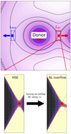Fig. B.1. Schematic diagram for the location of our computational domain and transition from a hydrostatic solution to Roche lob overflow. The top panel depicts the shape of the Roche-lobe equipotential surfaces, along with the approximate locations of our computational domains (rectangles) around Lin (red cross) and Lout (blue cross). The arrows indicate the direction of overflowing gas. The diagram is drawn not to scale. The bottom panels depict the density change, with denser regions shown in darker colors, during the transition from a contact binary in hydrostatic equilibrium to overflow by imposing an outflow boundary condition (BC) along the right x boundary. The dashed diagonal orange lines depict the shape of the RL.

To resolve the overflowing stream and stably maintain its steady state deep inside the donor, we adaptively refined the cells with $\stackrel{\sim }{\rho }>{10}^{-3}$. The base-level resolution and refinement levels (up to 2 levels for γ = 1 and 3 levels for γ = 5/3) were determined to reach the convergent gas morphology and mass overflow rate. At the base-level, we placed 10 − 20 cells across the width of the stream crossing over the Lagrangian point, which increased by a factor of 2 − 4 at the highest level of refinement in each direction. This resolution at the highest level of refinement corresponds to at least 30 − 50 cells and 10 − 30 cells per pressure scale height (P/(dP/dR)) inside the donor for the adiabatic and isothermal cases, respectively. We performed resolution tests for the equal-mass, L_in adiabatic and isothermal cases by varying the resolution at the highest level of refinement, and we confirmed that the resolution used in the simulations presented in the paper yield converged results.

We adopted a simple Γ equation of state, P = (Γ − 1)u with Γ = 5/3 for γ = 5/3, and an isothermal equation of state for γ = 1.

B.2. From a contact binary to RL overflow – Mapping, relaxation, and boundary conditions

We first mapped the solution for a contact binary onto a 3D domain using Eq. (A.10) for γ = 5/3 or Eq. (A.13) for γ = 1, and then relaxed it without the Coriolis force. The solution for γ = 5/3 has a sharp edge at which $\stackrel{\sim }{\rho }=0$. For numerical stability, we impose a density floor of $\stackrel{\sim }{\rho }={10}^{-7}$, effectively extending the edge only down to this floor value. In addition, the rest of the domain is filled with low-density gas at the floor value, with the pressure determined by the polytropic relation. The solution for γ = 1 does not have a sharp edge. But we still impose a density floor of 10⁻¹⁰.

To efficiently damp the motion of gas during the relaxation phase and in the transition phase once the gas begins to flow, we employed an isotropic viscosity, which depends on time and location, such that

$$\begin{array}{c}\hfill \nu (\stackrel{\sim }{t},\stackrel{\sim }{r})=\frac{tanh[-3(sign(\stackrel{\sim }{x})\stackrel{\sim }{r}+1)]+1}{2}[{\nu }_0(tanh(-{\stackrel{\sim }{t}}^2/t_{\nu })+1)+{\nu }_{\min }],\end{array}$$(B.1)

where $\stackrel{\sim }{r}$ is the radial distance from the Lagrangian point. The first term determines the location dependence of ν. The first term is of order unity in the inside of the donor ($\stackrel{\sim }{r}>1$ and $sign(\stackrel{\sim }{x})=-1$), which approaches zero toward the accretor ($sign(\stackrel{\sim }{x})=1$). The second term considers the temporal evolution of ν such that the viscosity deceases from ν₀ to ν_min over a timescale of t_nu. To maintain reasonable step-sizes, we employed super-time-stepping method with the second order Runge-Kutta-Legendre integrator. We took ν₀ ≃ 0.1 − 0.5, t_ν = 3 − 4, and v_min = 10⁻² − 10⁻³, depending on q and whether it is for the L_in or L_out point. These values for viscosity, which were chosen based on comprehensive test simulations, are initially high enough to efficiently damp the transient motion of gas in a transition phase and then quickly drops so that the overflowing rate reaches a steady state. If the viscosity remains high for too long, the overflow rate tends to continuously decrease, rather than reaching a steady state solution.

Under these conditions, relaxation usually took around $\stackrel{\sim }{t}\simeq 2-3$ to damp numerical oscillations of gas within the domain. The Mach number of fully relaxed gas was ≲10⁻² in the domain. The boundary conditions at this stage were given such that the ghost cells were filled, following the analytic solutions (Eq. (A.10) or (A.13)) if the “real” gas initially touched the boundary, and with zero-gradient extrapolation for the rest of the boundaries.

Once the gas was fully relaxed, we applied the outflow boundary condition to the positive x-boundary (toward the accretor) and included the Coriolis force, while the density floor values and the rest of the boundary conditions remained the same. This effectively emulates the RL overflow in a semi-detached binary by driving gas outflows beyond the Lagrangian point from an overfilling donor through the positive x-boundary. The transition from a contact binary to RL overflow is shown in the bottom panels in Fig. B.1. The transferring gas and the donor’s surface typically underwent a transition phase before reaching a steady state typically within $\stackrel{\sim }{t}\simeq 5-15$, which is sufficiently shorter than the duration of simulations ($\stackrel{\sim }{t}\gtrsim 50$ for q ≤ 1 and 25 − 30 for q > 1).

All Tables

All Figures

Fig. 1. Curvature of the gravitational (Roche) potential near the inner and outer Lagrangian points around the donor star. The middle panel depicts an overall shape of the Roche potential in a binary in the corotating frame. The inner and outer Lagrangian points of the donor, indicated by a violet star and magenta cross, respectively, are where our computational domain is located. The $\stackrel{\sim }{x}$ axis of the domain is aligned with the binary axis and the z axis is parallel to the binary orbit axis. The left panels illustrate the significantly steeper curvature and shallower potential depth – both perpendicular (top) and parallel (bottom) to the binary axis – near the inner Lagrangian point than the outer Lagrangian point for a system where the donor and accretor have comparable masses (for instance, stellar binaries). The right panels show the same quantities for a case where the donor mass is significantly smaller than the accretor mass (for example, stellar extreme mass ratio inspiral). In this case, similar to the comparable mass ratio case, the potential near the outer Lagrangian point exhibits shallower curvature. However, the depths become comparable. In fact, the depths become equal as the ratio of the donor mass to the accretor mass approaches zero. The curvature of the potential near the Lagrangian points is primarily determined by the coefficients of the quadratic terms in the Taylor expansion of the Roche potential (Eq. (2)).

In the text

Fig. 2. Trajectories of particles for a steady state solution of an equal-mass adiabatic case (left: without Coriolis force and middle: with Coriolis force) and an equal-mass isothermal case (right) in the midplane around the inner Lagrangian point, plotted over the density distribution. The particles are initially distributed following the same distribution of the initial density profile over a region with ${10}^{-3}\lesssim \stackrel{\sim }{\rho }\lesssim 20$ and their trajectories are integrated for $\stackrel{\sim }{t}\simeq 20$ since the flow reaches a steady state, assuming the particles are advected with the gas. Crosses at one end of the lines indicate the initial locations of the particles. We distinguish particles that reach beyond the Lagrangian point (yellow) from those that remain inside the donor (orange) over the integration duration.

In the text

Fig. 3. Shape and location of the sonic surface near the inner Lagrangian point. The 3D images of the binary near the Lagrangian point in the center show the orientation of the 2D plane in which the 2D distribution of Mach number is depicted – mid- (top) and vertical (bottom) slices. The panels on the left show the distributions for the equal-mass adiabatic case, while those on the right correspond to the equal-mass isothermal case. In the panels showing the Mach number distribution, the dashed diagonal orange lines depict the shape of the Roche lobe.

In the text

Fig. 4. Vertical and lateral motion of overflowing stream, relative to the motion toward the accretor, in the plane normal to the binary axis and intersecting the Lagrangian point (magenta cross), with the Coriolis force. Gas with $\stackrel{\sim }{\rho }<{10}^{-3}$ (white background), which contributes negligibly to the overflowing stream, is masked out for better visualization. ${\stackrel{\sim }{v}}^i$ (i = x, y, z) is the ith velocity component relative to the Lagrangian point. In both cases – adiabatic (left) and isothermal (right), we assume an equal-mass binary. The hatched areas indicate the velocity ratios less than 0.05, suggesting that the gas may be assumed to be in hydrostatic equilibrium. The arrows show the overall motion of the stream.

In the text

Fig. 5. Angle of the transferring stream relative to the binary axis for adiabatic (left) and isothermal cases (right) in the presence of the Coriolis force. The angle is defined as $tan\theta =⟨{\stackrel{\sim }{v}}^{\mathit{y}}⟩/⟨{\stackrel{\sim }{v}}^x⟩$, where $⟨{\stackrel{\sim }{v}}^x⟩$ and $⟨{\stackrel{\sim }{v}}^{\mathit{y}}⟩$ are mass-weighted averages of ${\stackrel{\sim }{v}}^x$ and ${\stackrel{\sim }{v}}^{\mathit{y}}$ measured at the right x-boundary. The solid curves following the dots indicate the fitting formulae given in Eq. (3). The vertical solid gray lines indicate equal-mass binary. In the right panel, the dotted curves indicates the predictions of the tilt angle for the isothermal case by Lubow & Shu (1975).

In the text

Fig. 6. Ratio of the numerically estimated mass transfer rate $\dot{\stackrel{\sim }{M}}$ in the presence of the Coriolis force to the analytic estimates ${\dot{\stackrel{\sim }{M}}}_{\mathrm{analytic}}$ (Eq. (A.25) for for the adiabatic case (left) and Eq. (A.30) for the isothermal case (right)). The solid curves following the dots indicate the fitting formulae given in Eq. (A.2). The solid vertical gray lines indicate equal-mass binary. Note that no assumption for the overfilling factor is made for this comparison as the overfilling factor is a scaling factor (see Eqs. (A.25) and (A.30)). We refer to Fig. 9 for a comparison of $\dot{\stackrel{\sim }{M}}$ between Lin and Lout for a given overfilling factor.

In the text

Fig. 7. Comparison between numerical (orange) and analytic solutions (gray lines). We compare density $\stackrel{\sim }{\rho }$ (top row), velocity toward the accretor ${\stackrel{\sim }{v}}^x$ (middle row), and $\stackrel{\sim }{\rho }{\stackrel{\sim }{v}}^x$ (bottom row) from our simulations along the $\stackrel{\sim }{\mathit{y}}$ axis intersecting the inner Lagrangian point ($\stackrel{\sim }{\mathit{y}}=0$) to the corresponding analytic solutions. We consider equal-mass binaries for both adiabatic – without (left column) and with (middle column) the Coriolis force – and isothermal cases with the Coriolis force (right column).

In the text

Fig. 8. Dynamical term ℱ1 accounting for the stream cross-section, hydrodynamical effects and the Coriolis force (colored lines) in the calculation of the mass transfer rate. In the bottom panel, the solid gray line represents the term only accounting for the potential geometry for the inner Lagrangian point introduced in Ritter (1988), who also provided a fitting formula (dashed gray line). The thick colored lines show the improved dynamical term for the adiabatic (dot-dashed lines) and isothermal (dashed lines) cases and the Roche potential geometry for the inner (red) and outer (blue) Lagrangian points. The fitting formula (thinner solid lines), closely overlapping with the thicker lines, reproduces the factors within 2.5% across the full range of mass ratio considered.

In the text

Fig. 9. Onset of outflow through the outer Lagrangian point and the ratio of the mass transfer rate between the inner (Ṁin) and outer (Ṁout) Lagrangian points. The solid (dashed) lines represent the ratios predicted by the extension of Kolb & Ritter (1990) with (without) our correction factors. The star markers on the zero line indicate the characteristic relative overfilling factors at which outflow through the Lout point begins. The colored regions represent the range of overfilling factors for which outflow occurs through both Lagrangian points, as well as the maximum rate ratio over the range of parameters considered.

In the text

Fig. A.1. Quadratic coefficients (Eq. (2)) that determine the curvature of the Roche potential near the Lagrangian point along the binary axis (A, left) and in the plane normal to the binary axis (B and C, right). The three coefficients are related by B = −(A + 3)/2 and C = B + 1. The red (blue) line represents the coefficients for the inner (outer) Lagrangian point, as a function of the donor mass over the accretor mass. In both panels, a few examples of mass transferring systems are presented in three different mass ratio regimes such as stellar extreme mass ratio inspiral (EMRI), even though the boundaries among these regimes are not clearly defined.

In the text

	Fig. A.2. Ratio of one distance code unit (${\mathrm{\Omega }}^{-1}\sqrt{|\xi |}$) to the effective size of the donor Rd, as a function of the relative overfilling factor α, defined as α = (Rd − RL)/RL. Here, RL is the effective RL size. We consider the inner Lagrangian point for this conversion.
In the text

Fig. B.1. Schematic diagram for the location of our computational domain and transition from a hydrostatic solution to Roche lob overflow. The top panel depicts the shape of the Roche-lobe equipotential surfaces, along with the approximate locations of our computational domains (rectangles) around Lin (red cross) and Lout (blue cross). The arrows indicate the direction of overflowing gas. The diagram is drawn not to scale. The bottom panels depict the density change, with denser regions shown in darker colors, during the transition from a contact binary in hydrostatic equilibrium to overflow by imposing an outflow boundary condition (BC) along the right x boundary. The dashed diagonal orange lines depict the shape of the RL.

In the text

References

- Armitage, P. J., & Livio, M. 1996, ApJ, 470, 1024 [NASA ADS] [CrossRef] [Google Scholar]
- Belczynski, K., Kalogera, V., & Bulik, T. 2002, ApJ, 572, 407 [NASA ADS] [CrossRef] [Google Scholar]
- Belczynski, K., Ryu, T., Perna, R., et al. 2017, MNRAS, 471, 4702 [Google Scholar]
- Bisikalo, D. V., Boyarchuk, A. A., Chechetkin, V. M., Kuznetsov, O. A., & Molteni, D. 1998, MNRAS, 300, 39 [NASA ADS] [CrossRef] [Google Scholar]
- Bobrick, A., Davies, M. B., & Church, R. P. 2017, MNRAS, 467, 3556 [NASA ADS] [CrossRef] [Google Scholar]
- Burbidge, E. M., & Sandage, A. 1958, ApJ, 128, 174 [Google Scholar]
- Casares, J., Jonker, P. G., & Israelian, G. 2017, in Handbook of Supernovae, eds. A. W. Alsabti, & P. Murdin, 1499 [Google Scholar]
- Cehula, J., & Pejcha, O. 2023, MNRAS, 524, 471 [NASA ADS] [CrossRef] [Google Scholar]
- Chen, Z., Frank, A., Blackman, E. G., Nordhaus, J., & Carroll-Nellenback, J. 2017, MNRAS, 468, 4465 [NASA ADS] [CrossRef] [Google Scholar]
- Church, R. P., Dischler, J., Davies, M. B., et al. 2009, MNRAS, 395, 1127 [Google Scholar]
- de Mink, S. E., Langer, N., Izzard, R. G., Sana, H., & de Koter, A. 2013, ApJ, 764, 166 [Google Scholar]
- de Mink, S. E., Sana, H., Langer, N., Izzard, R. G., & Schneider, F. R. N. 2014, ApJ, 782, 7 [Google Scholar]
- de Vries, N., Portegies Zwart, S., & Figueira, J. 2014, MNRAS, 438, 1909 [NASA ADS] [CrossRef] [Google Scholar]
- Dickson, D. 2024, ApJ, 975, 130 [Google Scholar]
- Dorozsmai, A., & Toonen, S. 2024, MNRAS, 530, 3706 [NASA ADS] [CrossRef] [Google Scholar]
- D’Souza, M. C. R., Motl, P. M., Tohline, J. E., & Frank, J. 2006, ApJ, 643, 381 [CrossRef] [Google Scholar]
- Eggleton, P. 2006, Evolutionary Processes in Binary and Multiple Stars (Cambridge: Cambridge University Press) [Google Scholar]
- Ferraro, F. R., Sabbi, E., Gratton, R., et al. 2006, ApJ, 647, L53 [NASA ADS] [CrossRef] [Google Scholar]
- Ge, H., Hjellming, M. S., Webbink, R. F., Chen, X., & Han, Z. 2010, ApJ, 717, 724 [NASA ADS] [CrossRef] [Google Scholar]
- Hamers, A. S., & Dosopoulou, F. 2019, ApJ, 872, 119 [NASA ADS] [CrossRef] [Google Scholar]
- Han, Z., Podsiadlowski, P., Maxted, P. F. L., Marsh, T. R., & Ivanova, N. 2002, MNRAS, 336, 449 [Google Scholar]
- Hellier, C. 2001, Cataclysmic Variable Stars (Springer Praxis Books) [Google Scholar]
- Hjellming, M. S., & Webbink, R. F. 1987, ApJ, 318, 794 [Google Scholar]
- Huang, S.-S. 1966, ARA&A, 4, 35 [NASA ADS] [CrossRef] [Google Scholar]
- Hubová, D., & Pejcha, O. 2019, MNRAS, 489, 891 [Google Scholar]
- Ivanova, N., Justham, S., Chen, X., et al. 2013, A&ARv, 21, 59 [Google Scholar]
- Ivanova, N., Justham, S., & Ricker, P. 2020, Common Envelope Evolution [Google Scholar]
- Ivanova, N., Kundu, S., & Pourmand, A. 2024, ApJ, 971, 64 [NASA ADS] [CrossRef] [Google Scholar]
- Jackson, B., Arras, P., Penev, K., Peacock, S., & Marchant, P. 2017, ApJ, 835, 145 [NASA ADS] [CrossRef] [Google Scholar]
- Jermyn, A. S., Bauer, E. B., Schwab, J., et al. 2023, ApJS, 265, 15 [NASA ADS] [CrossRef] [Google Scholar]
- Joss, P. C., & Rappaport, S. A. 1984, ARA&A, 22, 537 [Google Scholar]
- Kadam, K., Motl, P. M., Marcello, D. C., Frank, J., & Clayton, G. C. 2018, MNRAS, 481, 3683 [Google Scholar]
- King, A. R. 1996, Ap&SS, 237, 169 [Google Scholar]
- Kippenhahn, R. 1969, A&A, 3, 83 [NASA ADS] [Google Scholar]
- Kippenhahn, R., & Meyer-Hofmeister, E. 1977, A&A, 54, 539 [NASA ADS] [Google Scholar]
- Kolb, U., & Ritter, H. 1990, A&A, 236, 385 [NASA ADS] [Google Scholar]
- Kopal, Z. 1959, Close Binary Systems (New York: Wiley) [Google Scholar]
- Kruszewski, A. 1967, Acta Astron., 17, 297 [NASA ADS] [Google Scholar]
- Lajoie, C.-P., & Sills, A. 2011, ApJ, 726, 67 [Google Scholar]
- Lanzafame, G., Belvedere, G., & Molteni, D. 2006, A&A, 453, 1027 [NASA ADS] [CrossRef] [EDP Sciences] [Google Scholar]
- Lubow, S. H., & Shu, F. H. 1975, ApJ, 198, 383 [NASA ADS] [CrossRef] [Google Scholar]
- Marchant, P., Pappas, K. M. W., Gallegos-Garcia, M., et al. 2021, A&A, 650, A107 [NASA ADS] [CrossRef] [EDP Sciences] [Google Scholar]
- McCrea, W. H. 1964, MNRAS, 128, 147 [Google Scholar]
- Meyer, F., & Meyer-Hofmeister, E. 1983, A&A, 121, 29 [NASA ADS] [Google Scholar]
- Misra, D., Fragos, T., Tauris, T. M., Zapartas, E., & Aguilera-Dena, D. R. 2020, A&A, 642, A174 [NASA ADS] [CrossRef] [EDP Sciences] [Google Scholar]
- Nariai, K., & Sugimoto, D. 1976, PASJ, 28, 593 [NASA ADS] [Google Scholar]
- Nelson, C. A., & Eggleton, P. P. 2001, ApJ, 552, 664 [NASA ADS] [CrossRef] [Google Scholar]
- Nomoto, K. 1982, ApJ, 253, 798 [Google Scholar]
- Norton, A. J., Butters, O. W., Parker, T. L., & Wynn, G. A. 2008, ApJ, 672, 524 [NASA ADS] [CrossRef] [Google Scholar]
- Oka, K., Nagae, T., Matsuda, T., Fujiwara, H., & Boffin, H. M. J. 2002, A&A, 394, 115 [NASA ADS] [CrossRef] [EDP Sciences] [Google Scholar]
- Olejak, A., Stegmann, J., de Mink, S. E., et al. 2025, ArXiv e-prints [arXiv:2503.21995] [Google Scholar]
- Paczyński, B. 1965, Acta Astron., 15, 89 [NASA ADS] [Google Scholar]
- Paczyński, B. 1971, ARA&A, 9, 183 [Google Scholar]
- Paczyński, B., & Sienkiewicz, R. 1972, Acta Astron., 22, 73 [NASA ADS] [Google Scholar]
- Pavlovskii, K., & Ivanova, N. 2015, MNRAS, 449, 4415 [Google Scholar]
- Pavlovskii, K., Ivanova, N., Belczynski, K., & Van, K. X. 2017, MNRAS, 465, 2092 [Google Scholar]
- Paxton, B., Cantiello, M., Arras, P., et al. 2013, ApJS, 208, 4 [Google Scholar]
- Paxton, B., Marchant, P., Schwab, J., et al. 2015, ApJS, 220, 15 [Google Scholar]
- Podsiadlowski, P., Rappaport, S., & Pfahl, E. D. 2002, ApJ, 565, 1107 [NASA ADS] [CrossRef] [Google Scholar]
- Prendergast, K. H., & Burbidge, G. R. 1968, ApJ, 151, L83 [Google Scholar]
- Rajamuthukumar, A. S., Bauer, E. B., Justham, S., et al. 2024, ArXiv e-prints [arXiv:2411.08099] [Google Scholar]
- Reichardt, T. A., De Marco, O., Iaconi, R., Tout, C. A., & Price, D. J. 2019, MNRAS, 484, 631 [NASA ADS] [CrossRef] [Google Scholar]
- Ritter, H. 1988, A&A, 202, 93 [NASA ADS] [Google Scholar]
- Roche, E. 1873, Mem. Acad. Sci. Montpellier, 8, 235 [Google Scholar]
- Sana, H., de Mink, S. E., de Koter, A., et al. 2012, Science, 337, 444 [Google Scholar]
- Sana, H., de Koter, A., de Mink, S. E., et al. 2013, A&A, 550, A107 [NASA ADS] [CrossRef] [EDP Sciences] [Google Scholar]
- Sandage, A. R. 1953, AJ, 58, 61 [Google Scholar]
- Scherbak, P., Lu, W., & Fuller, J. 2025, ArXiv e-prints [arXiv:2505.21264] [Google Scholar]
- Schneider, F. R. N., Ohlmann, S. T., Podsiadlowski, P., et al. 2019, Nature, 574, 211 [Google Scholar]
- Stone, J. M., Gardiner, T. A., Teuben, P., Hawley, J. F., & Simon, J. B. 2008, ApJS, 178, 137 [NASA ADS] [CrossRef] [Google Scholar]
- Stone, J. M., Tomida, K., White, C. J., & Felker, K. G. 2020, ApJS, 249, 4 [NASA ADS] [CrossRef] [Google Scholar]
- Tauris, T. M., & van den Heuvel, E. P. J. 2006, in Compact stellar X-ray Sources, eds. W. H. G. Lewin, & M. van der Klis, 39, 623 [Google Scholar]
- Tauris, T. M., & van den Heuvel, E. P. J. 2023, Physics of Binary Star Evolution. From Stars to X-ray Binaries and Gravitational Wave Sources (Princeton: Princeton University Press) [Google Scholar]
- Temmink, K. D., Pols, O. R., Justham, S., Istrate, A. G., & Toonen, S. 2023, A&A, 669, A45 [NASA ADS] [CrossRef] [EDP Sciences] [Google Scholar]
- Thomas, D. M., & Wood, M. A. 2015, ApJ, 803, 55 [NASA ADS] [CrossRef] [Google Scholar]
- Toyouchi, D., Hotokezaka, K., Inayoshi, K., & Kuiper, R. 2024, MNRAS, 532, 4826 [NASA ADS] [CrossRef] [Google Scholar]
- van den Heuvel, E. P. J., Portegies Zwart, S. F., & de Mink, S. E. 2017, MNRAS, 471, 4256 [Google Scholar]
- van Son, L. A. C., de Mink, S. E., Renzo, M., et al. 2022, ApJ, 940, 184 [NASA ADS] [CrossRef] [Google Scholar]
- Wang, C., & Ryu, T. 2024, ArXiv e-prints [arXiv:2410.10314] [Google Scholar]
- Warner, B. 1995, Cataclysmic Variable Stars,, 28 (Cambridge: Cambridge University Press) [Google Scholar]
- Whelan, J., & Iben, I., Jr 1973, ApJ, 186, 1007 [Google Scholar]
- Woods, T. E., & Ivanova, N. 2011, ApJ, 739, L48 [NASA ADS] [CrossRef] [Google Scholar]
- Zhilkin, A. G., & Bisikalo, D. V. 2010, Astron. Rep., 54, 840 [Google Scholar]