| Issue |
A&A
Volume 702, October 2025
|
|
|---|---|---|
| Article Number | A113 | |
| Number of page(s) | 15 | |
| Section | Extragalactic astronomy | |
| DOI | https://doi.org/10.1051/0004-6361/202555679 | |
| Published online | 17 October 2025 | |
The slow evolution of dark matter halos from cusp to core naturally produces extended stellar core-like distributions
1
Instituto de Astrofísica de Canarias, La Laguna, Tenerife, E-38200, Spain
2
Departamento de Astrofísica, Universidad de La Laguna, Spain
3
CeBio y Departamento de Ciencias Básicas, Universidad Nacional del Noroeste de la Prov. de Buenos Aires, UNNOBA, CONICET, Roque Saenz Peña 456, Junin, Argentina
⋆ Corresponding authors: This email address is being protected from spambots. You need JavaScript enabled to view it.
, This email address is being protected from spambots. You need JavaScript enabled to view it.
, This email address is being protected from spambots. You need JavaScript enabled to view it.
Received:
27
May
2025
Accepted:
14
August
2025
Abstract
Motivated by the observation of extended stellar cores in dark matter (DM)-dominated dwarf galaxies, this study investigates a simple mechanism by which stellar cores can form as a result of DM halo expansion. Several non-CDM models predict that the DM distribution thermalizes over time, transforming initially cuspy halos into cores. This transformation weakens the gravitational potential, allowing the stellar component to expand and form diffuse, core-like structures. Using analytical models and adiabatic invariants, we examine stellar systems with purely tangential, purely radial, and isotropic orbits evolving under a slowly changing potential. Across a wide range of initial and final conditions, we find that stellar cores form relatively easily, though their properties depend sensitively on these conditions. Orbit types preserve their nature during the DM halo expansion: tangential and radial orbits remain so, while isotropic orbits remain nearly isotropic in the central regions. Systems with circular orbits develop stellar cores when the initial stellar density logarithmic slope lies between −0.5 and −1.2, whereas radial systems do not form cores. Isotropic systems behave similarly to tangential ones, producing cores that are isotropic in the center but develop increasing radial anisotropy outward; the anisotropy parameter β grows from 0.07 at the core radius to ∼0.5 at three core radii. The theoretical and observational literature suggests initial DM profiles with steep slopes and stellar distributions that are shallower and isotropic at the center. Given these conditions, the mechanism predicts stellar cores with radii at least 40% that of the DM core and inner logarithmic slopes shallower than 0.6.
Key words: galaxies: dwarf / galaxies: evolution / galaxies: halos / galaxies: stellar content / dark matter
© The Authors 2025
 Open Access article, published by EDP Sciences, under the terms of the Creative Commons Attribution License (https://creativecommons.org/licenses/by/4.0), which permits unrestricted use, distribution, and reproduction in any medium, provided the original work is properly cited.
This article is published in open access under the Subscribe to Open model. This email address is being protected from spambots. You need JavaScript enabled to view it. to support open access publication.
1. Introduction
Although faint low-surface-brightness galaxies with extended stellar distributions have been known since the 1980s (Binggeli et al. 1984; Caldwell & Bothun 1987), a new generation of deep surveys is disclosing a large number of them. They receive several names depending on the technique of observation and galaxy mass, including ultra-diffuse galaxies (UDGs; e.g., van Dokkum et al. 2015; Román & Trujillo 2017; Conselice 2018; Müller et al. 2018; Trujillo 2021) or ultra-faint galaxies (UFDs; e.g., Simon 2019; Richstein et al. 2024; Arias et al. 2025). They tend to be satellites of nearby larger galaxies, but this is probably an observational bias given the difficulties in detecting faint low-surface-brightness sources at large distances in low-density fields. One of their more conspicuous features is the lack of a clear concentration of stars marking the center of the stellar distribution not obvious at first sight. An extreme case is the galaxy Nube (Montes et al. 2024), with a large half-mass radius (6.9 kpc) and a mass distribution with a central plateau of low mass surface density (∼1 M⊙ pc−2), but there are many other examples (Mihos et al. 2015; Carlsten et al. 2022; Arias et al. 2025). According to the standard picture, these spread-out stellar distributions could be caused by stellar feedback in low-mass dark matter (DM) halos (e.g., Di Cintio et al. 2017; Campbell et al. 2017; Lazar et al. 2020). However, the presence of these stellar density plateaus or cores have been detected in objects too small for the stellar feedback mechanism to operate Sánchez Almeida et al. (2024b). The question arises of whether mechanisms other than the stellar feedback can also produce the observed extended stellar cores.
Here we analyze a conceptually simple physical mechanism to produce spread-out stellar cores in DM-dominated halos with stars. If internal processes make the DM evolve with time to create a core, then the gravitational force that maintains the stellar system drops. The stellar system expands dragged along by the expansion of DM creating a diffuse system of stars with a core. A number of physical models of DM going beyond CDM produce the described slow expansion; for instance, self-interacting DM (SIDM; Spergel & Steinhardt 2000) turns cusps into cores within a timescale of the order of the Hubble time (tH; e.g., Outmezguine et al. 2023). The timescale for the evolution of warm DM halos is similar to the formation of CDM halos, and so, also around tH (Colín et al. 2000; Bode et al. 2001). Fuzzy DM (Schive et al. 2014), self-interacting fuzzy DM (Indjin et al. 2025), and Bose-Einstein condensates (Delgado & Muñoz Mateo 2023) all lead to the formation of cores on timescales shorter than in SIDM, but still longer than the dynamical timescale (e.g., Mocz et al. 2017). Fermionic DM evolves on cosmological timescales (Argüelles et al. 2023), whereas late-time DM decay (Chu & Garcia-Cely 2018) leads to the gradual formation of DM cores at late times. These are just illustrative examples, however, we stress that the mechanism is independent of the actual DM model ultimately responsible for the expansion. In a sense, it is inverse to the adiabatic contraction suffered by CDM halos early on, when the sinking of baryons toward the center of the potential drives the compaction of the DM halos (Blumenthal et al. 1986; Gnedin et al. 2004). In our case the expansion of the DM halo drives the expansion of the stellar system.
Our work aims to show that the hypothetical mechanism seems to work in practice. We use a number of simplified spherically symmetric analytical models showing that the expansion of almost any DM halo giving rise to a core drags along the preexisting stars, often producing a core-like structure in the inner stellar distribution. Depending on the initial conditions, this core is comparable in size with the DM core, a fact consistent with the observations of some early-type dwarf galaxies having the two radii available (Sánchez Almeida et al. 2024a,b, 2025).
Since the underlying assumption is that variations in the DM distribution occur slowly, on a timescale much longer than the period of stellar orbits, action variables remain constant, simplifying the study of the process (e.g., Binney & Tremaine 2008). The final stellar distribution depends only on the initial and final distribution of DM and on the initial distribution of stars, being independent of the actual pathway from initial to final.
The paper is organized as follows: Sect. 2 describes three types of analytical spherically symmetric systems with different and extreme velocity anisotropies covering all possibilities, from purely tangential to purely radial orbits. Section 2.1 treats models with circular orbits that have only tangential velocities, characterized by a velocity anisotropy parameter β = −∞ (β is defined in Eq. (1)). In general, the action variables are not analytical, however, the Henon’s isochrone potential (Henon 1959b; Binney & Tremaine 2008) is especially useful in our context because the action variables can be expressed in closed analytical form. We use it in Sect. 2.2 to study initially isotropic stellar orbits (β = 0). Finally, purely radial orbits are considered in Sect. 2.3 (β = 1). (Appendix A also shows how numerically handle arbitrary potentials.) We discuss the behavior under a broad range of initial and final conditions, finding that stellar cores are easily produced for a wide range of initial conditions. However, the properties of the induced stellar cores depend on the initial conditions. Thus, in Sect. 3 we revise the existing literature on the initial conditions to be expected, including the DM and stellar mass density distributions as well as the velocity anisotropy of the stars. Appendix C analyzes the expected relative half-mass radii of DM and stars when halos first formed in the early Universe. The constraints set by the expected initial conditions on the resulting stellar core-like structures are discussed in Sect. 4. Finally, the results and conclusions to be extracted from our simple modeling are summarized in Sect. 5. All the analysis neglects the self-gravity of the stars, which is well justified for some objects (e.g., Sánchez Almeida et al. 2024b) but not in general. The impact of the self-gravity of the stars is briefly addressed in Sect. 5. Appendix B addresses why the relative expansion of the stellar cores induced by the mechanism agrees with the expansion of the DM core.
2. Analytical models to treat the adiabatic expansion of the stellar system
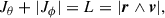
We consider three types of spherically symmetric systems with different and extreme velocity anisotropies covering all possibilities. As it was mentioned in the introduction (Sect. 1), the assumed slow variation in the DM distribution makes it possible to describe the time evolution using adiabatic invariants, which remain conserved throughout the process. The contribution of the stars to the potential is in all cases assumed to be negligible. Thus, our modeling is meant to describe dwarf galaxies fully dominated by DM at all times. The main difference between models is the anisotropy of the stellar orbits with are usually described using the anisotropy parameter, β, defined as
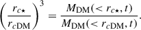
 (1)
(1)
with σt2 the dispersion of tangental velocities and σr2 the dispersion of radial velocities at a given radial distance (e.g., Binney & Tremaine 2008). Stellar systems with circular orbits have σr2 = 0 and so are characterized by β = −∞, systems with isotropic orbits have β = 0, and systems with pure radial orbits have β = 1. They are treated in Sects. 2.1, 2.2, and 2.3, respectively. The general case of arbitrary potential and β is put forward in Appendix A. As it was mentioned above, the self-gravity of the stars is neglected, but the impact of the self-gravity of the stars is briefly considered in Sect. 5.
2.1. Circular stellar orbits in arbitrary spherical potentials
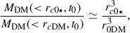
Here, we consider spherically symmetric stellar systems with purely tangential orbits living in an externally imposed potential which is time dependent but always spherical. Since the potential is spherical and there are no initial radial velocities, the initial orbits are circular and depend only on the radial coordinate r. In this idealized situation, the gravitational forces are perfectly balanced with the centrifugal forces so that
 (2)
(2)
with v⋆ the circular velocity of the stars and MDM(< r, t) the DM mass internal to r,
 (3)
(3)
which is assumed to be distributed with a volume density ρDM(r, t). As usual, G stands for the gravitational constant. In the case of circular orbits, the radial invariant is zero (Eq. (A.1), with rmin = rmax = r). Since the adiabatic invariants are conserved, it is also zero in the final orbits, so that the initial circular orbits remain circular, and the balance given by Eq. (2) is maintained at any time t. The angular momentum of the orbits is also conserved, so that the plane of each orbit remains invariant. Thus, a star starting at t0 with an orbit of radius r0 and ending at t with an orbit of radius r has to comply with the condition
 (4)
(4)
The stellar mass is also conserved during expansion, therefore, if a stellar shell at t0 becomes another shell at t then
 (5)
(5)
with ρ⋆(r, t) the density in the shell at r and t and Δr0 and Δr the widths of the initial and final shells. Given Eqs. (2) and (4), the radii of the orbits have to scale as
 (6)
(6)
which also sets the ratio between the width of the shells used in Eq. (5),
![Mathematical equation: $$ \begin{aligned}&\Delta r \left[M_{\rm DM}(<r,t)+4\pi r^3\rho _{\rm DM}(r,t)\right] = \nonumber \\&\qquad \Delta r_0 \left[M_{\rm DM}( < r_0,t_0)+4\pi r_0^3\rho _{\rm DM}(r_0,t_0)\right]. \end{aligned} $$](/articles/aa/full_html/2025/10/aa55679-25/aa55679-25-eq7.gif) (7)
(7)
Equations (5), (6), and (7) provide the relationship between the initial distribution of stars at t0 and the final one,
![Mathematical equation: $$ \begin{aligned} \rho _\star (r,t) = \rho _\star (r_0,t_0)\times \left[\frac{M_{\rm DM}(<r,t)}{M_{\rm DM}(<r_0,t_0)}\right]^2\times \nonumber \\ \left[\frac{M_{\rm DM}(<r,t)+4\pi r^3\rho _{\rm DM}(r,t)}{M_{\rm DM}( < r_0,t_0)+4\pi r_0^3\rho _{\rm DM}(r_0,t_0)}\right],\end{aligned} $$](/articles/aa/full_html/2025/10/aa55679-25/aa55679-25-eq8.gif) (8)
(8)
once the initial and final distribution of DM are set. Specific examples are given in Sect. 2.1.2.
2.1.1. Densities following power laws
The inner parts of the density profiles used to represent DM and stellar distributions are often power laws, including the Navarro–Frenk–White (NFW; Navarro et al. 1997) profile characteristic of CDM halos, the polytropes representing self-gravitating systems of maximum entropy (Plastino & Plastino 1993; Sánchez Almeida et al. 2020), the early DM halos (see Sect. 3), as well the abc profiles commonly used to model mass density profiles in galaxies (Hernquist 1990; Merritt et al. 2006),
![Mathematical equation: $$ \begin{aligned} \rho (r) = \frac{\rho _{\rm s}}{(r/r_{\rm s})^c\,\left[1+(r/r_{\rm s})^a\right]^{(b-c)/a}}. \end{aligned} $$](/articles/aa/full_html/2025/10/aa55679-25/aa55679-25-eq9.gif) (9)
(9)
This abc profile is defined by a characteristic density and radius (ρs and rs, respectively) and three exponents (a, b, and c). The coefficient c sets the inner logarithmic slope of the profile since
 (10)
(10)
If the initial and final DM profiles as well as the initial stellar distribution are of this kind, then the final stellar profile is also a power law whose slope is
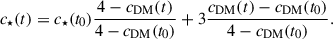 (11)
(11)
The previous expression considers that the inner slope of the DM, cDM(t), and the stars, c⋆(t), vary with time, and it can be derived from Eqs. (3) and (8). In the case of interest, the DM profile ends up with a core, i.e., cDM(t) = 0. Then the stars also end up with an inner core, c⋆(t) = 0, when
 (12)
(12)
Note also that according to Eq. (11), the final slope of the stars may be positive, c⋆(t) < 0, provided the difference of initial inner slopes between stars and DM is large enough,
 (13)
(13)
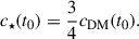
A positive final stellar slope implies the possibility of generating an inner depresion in the stellar distribution due to the expansion of the DM halo. In case the initial DM and stellar profiles have the same inner slope, c⋆(t0) = cDM(t0), then the final stellar slope is positive but much smaller than the original one,
 (14)
(14)
In the case of an initial NFW distribution, cDM(t0) = 1 and therefore c⋆(t) = 1/3. All the above properties are illustrated in Sect. 2.1.2.
2.1.2. Examples of systems with circular orbits
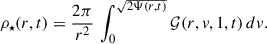
We have used Eqs. (3), (6), and (8), plugging in specific density profiles, to see the effect on the stars of the DM halo expansion. Figure 1a is used for reference and illustrates the physical process. The DM halo begins as a NFW profile (initial a, b, cDM[t0] = 1, 3, 1) and ends as a cored abc profile where only the inner slope has changed (final a, b, cDM[t] = 1, 3, 0). The final total mass has been scaled to be equal to the initial one. The initial stellar profile is also an abc profile with the inner slope tuned so that at the end it reaches a stellar profile with a perfect core (initial a, b, c⋆[t0] = 1, 3, 0.75; see Eq. (12)). The initial (dashed red line) and final (solid red line) DM profiles as well as for the initial stellar density profile (dashed blue line), all are assumed to have the same scale radius rs. To quantify the relative expansion between DM and stars, we use a core radius rc defined as the radius where the logarithmic slope of the profile reaches the mean between the maximum and the minimum logarithmic slopes, which are well defined in abc profiles (Eq. (9)). Explicitly, rc follows from
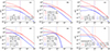 |
Fig. 1. Examples of the impact of the DM core formation (from the initial dashed red lines to the final solid red lines) on the formation of a stellar core (the solid blue lines) evolving from an originally concentrated stellar distribution (the dashed blue lines). The vertical dotted lines indicate the radius of the formed cores in DM (red) and stars (blue). The initial stars are assumed to follow circular orbits. For details on the types of profiles represented in the different panels, see Sect. 2.1.2. Arbitrary global scale factors affect both densities and radii. |
![Mathematical equation: $$ \begin{aligned} \frac{d\log \rho (r_{\rm c})}{d\log r}=\frac{1}{2}\left[\frac{d\log \rho (r)}{d\log r}\Big |_{\rm max}+\frac{d\log \rho (r)}{d\log r}\Big |_{\rm min}\right]. \end{aligned} $$](/articles/aa/full_html/2025/10/aa55679-25/aa55679-25-eq15.gif) (15)
(15)
As Fig. 1a shows, the final stellar distribution (solid blue line; from Eq. (8)) has a core produced by the DM expansion (vertical dotted blue line) similar in size to the final DM profile (vertical dotted red line). For the sake of representation, the stellar mass is assumed to be a hundredth of the DM mass, but this scaling is irrelevant provided the stellar mass is negligible with respect to the DM mass. The final DM and stellar profiles show almost exactly the same rc, so that the stellar core is a fair representation of the extent of the DM core.
Figure 1b is identical to Fig. 1a except that the initial stellar distribution has a characteristic scale rs ten times smaller. In this case the stellar core resulting from the expansion is 5 times smaller than the final DM core. The original difference has been reduced but not much. The reason why is analyzed in Appendix B.
Figure 1c is similar to Fig. 1a except for the inner slope of the initial DM profile, cDM(t0) = 1.5, chosen to be close to the primitive DM halos (see Sect. 3), and for the initial inner slope of the stars, chosen to be c⋆(t0) = 1. In addition, the coefficient a, which sets the shape of the transition between centers and outskirts in abc profiles, was set to two in the final DM density profile. Note that the inner slope of the final stellar distribution has become slightly positive, in agreement with Eq. (13).
We also tried three other types of profiles relevant for the work. The first one is shown in Fig. 1d and corresponds to the evolution of an initial NFW profile to a piecewise profile having an inner Plummer-Schuster profile1 and the outskirts of the original NFW profile. This kind of evolution is expected in models of DM where the DM particles also interact through forces besides gravity that allow them to collide and thermalize, thus creating an inner core (Robertson et al. 2021; Sánchez Almeida & Trujillo 2021; Sánchez Almeida 2025). In this particular case, the initial distribution of stars is assumed to be more concentrated than the DM and the system evolves to produce a stellar core around five times smaller than the DM core. The radii where the two pieces merge to form the final DM profile is taken to be three times the characteristic scale of the initial NFW DM halo.
Figure 1e includes an initial exponential stellar distribution, i.e., lnρ⋆ ∝ −r, with the length scale of the exponential much smaller than the scale of the initial DM profile. The expansion of DM creates an inner drop in the stellar mass distribution.
Finally, Fig. 1f shows the effect of DM core formation when the DM is described by a Henon’s isochrone potential. It is relevant for the present work because the adiabatic invariants in a Henon’s potential are analytical, thus, it allows the analytical study of systems with a wide range of velocity anisotropies. We take advantage of this in Sect. 2.2 to represent stars with isotropic velocities. The functional form of the Henon’s isochrone gravitational potential is simple (Henon 1959b,a; Hénon 1960; Binney & Tremaine 2008),
 (16)
(16)
where riso corresponds to a scale length and A2 = riso2 + r2. The density profile that generates the isochrone potential is (e.g., Binney & Tremaine 2008)
![Mathematical equation: $$ \begin{aligned} \rho (r) \, = M_{\rm iso} \left[ \frac{3(r_{\rm iso}+A) A^2 - r^2(r_{\rm iso}+3A)}{4\pi (r_{\rm iso} + A)^3 A^3} \right]. \end{aligned} $$](/articles/aa/full_html/2025/10/aa55679-25/aa55679-25-eq17.gif) (17)
(17)
The symbol Miso in Eqs. (16) and (17) stands for the total mass of the density associated with the potential. The density given by Eq. (17) has a core that vanishes in the limit riso → 0, and that can be made arbitrarily large increasing riso. Small riso has been used to represent the initial DM and stellar profiles in Fig. 1f; the dashed red and blue lines, respectively. The generation of the DM core by increasing riso (the solid red line) induces a stellar core (the solid blue line) that is, however, significantly smaller (compare the vertical dotted blue and red lines).
The density profiles in Fig. 1 just provide a glimpse of the effect the DM expansion induces on the stellar distribution. In order to get a more general picture, we carried out a series of simulations varying the properties of the stellar profile for a constant DM density profile variation (same starting and end DM profiles). The results are shown in Fig. 2. Each color represents the effect on the stellar distribution of a single pair of initial–final DM profiles. The actual values are given in the inset next to the top panel. Two parameters are used to characterize the expansion; the ratio between the stellar and DM core radii (Fig. 2, top panel) and the final inner slope of the resulting stellar profile (Fig. 2, bottom panel). Both parameters are represented against the initial inner slope of the stellar distribution. The main results are: (1) if the initial DM is described by a NFW profile, then the final stellar density profile develops a core-like feature (i.e., c⋆ Final ≡ c⋆[t]∼0) provided the initial stellar distribution has an inner slope in the range between 0.5 and 1.2 (i.e., c⋆ Initial ≡ c⋆[t0]∈[0.5, 1.2]). (2) The final stellar distribution develops a sort of inner dip or region deprived of stars when the initial stellar inner slope is well below the 0.5 limit. (3) The final stellar to DM core radius ratio scales with the initial ratio between the characteristic sizes of DM and stellar distributions, so that the process produces similar DM and stellar cores if the original distributions were of similar in size. In other words, the expansion rate of the DM is similar to the expansion rate it induces on the stars (see Appendix B for a detailed explanation). Thus, the process of DM expansion can also produce stellar cores smaller and larger than the DM cores depending on the initial conditions.
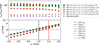 |
Fig. 2. Summary of the effect of the DM halo expansion on the stellar distribution when the orbits are circular (β = −∞). Two parameters are used to characterize the result: the ratio between the stellar and DM cores (top panel) and the final inner slope of the resulting stellar profile (bottom panel). Both are represented against the initial inner slope of the stellar distribution. The inset next to the top panel describes the initial and final DM profiles, with a, b, cDM referring to the parameters defining the ρabc profiles in Eq. (9). The solid black line labeled “Theory” in the bottom panel represents Eq. (11). The vertical dashed lines mark the initial cDM and follows the same color code as the upper panel. For further details, see Sect. 2.1.2. The region shaded in gray represents the approximate location of an observed stellar core. |
2.2. Initially isotropic stellar orbits in a Henon’s isochrone potential
Henon’s isochrone potential is defined in Eq. (16). The parameter riso controls its shape, which can go from the Kepler potential produced by a point mass (∝r−1 when riso → 0) to the harmonic potential characteristic of a system with constant mass density (∝r2 when riso → ∞). Thus, the density profile that generates the isochrone potential, given in Eq. (17), has a plateau when r ≪ riso and becomes a power law (∝r−4) when r ≫ riso (e.g., Binney & Tremaine 2008).
Here we consider a dynamical process in which a distribution of stars evolves under the effect of a changing isochrone potential. We assume an initial stellar phase-space distribution F(r, v, t0), which is a stationary distribution corresponding to an initial value riso(t0). The symbol v stands for the velocity vector. If the parameter riso changes slowly into a final value riso(t), the stellar distribution evolves into a corresponding final distribution F(r, v, t), which is a stationary distribution corresponding to another isochrone potential. Our aim is to determine the form of the final stellar distribution F(r, v, t), so that the final stellar density can be computed as
 (18)
(18)
If one expresses the initial star distribution as a distribution function (DF) of the action variables, then (e.g., Binney & Tremaine 2008)
 (19)
(19)
where 𝒟 is the DF providing the number of stars having actions in the ranges (Jr, Jr + dJr), (Jθ, Jθ + dJθ), and (Jϕ, Jϕ + dJϕ). The key fact used to determine the final star distribution is that, for a slowly changing potential, Jr, Jθ, and Jϕ are conserved, therefore, 𝒟(Jr, Jθ, Jϕ) is also conserved, and the final stellar distributions becomes
 (20)
(20)
We use r′ and v′ rather than r and v to evidence that the relation between the action variables and the position and velocity is not the same at t0 and t, even though Jr, Jθ, and Jϕ are time invariant. In the case of the Henon’s isochrone potential, the action variables can be written in closed analytical form in terms of the total energy, E, the total angular momentum, L, and one of the components of the angular momentum, Lz (Saha 1991; Binney & Tremaine 2008),
![Mathematical equation: $$ \begin{aligned} J_r&= \frac{GM_{\rm iso}}{\sqrt{-2E}} - \frac{1}{2} \left[ L + \sqrt{L^2 + 4G M_{\rm iso} r_{\rm iso}} \right], \end{aligned} $$](/articles/aa/full_html/2025/10/aa55679-25/aa55679-25-eq21.gif) (21)
(21)
 (22)
(22)
 (23)
(23)
Assuming isotropic velocities for the initial phase-space stellar DF, then the initial DF depends on r and v only through the energy (e.g., Binney & Tremaine 2008) so that
![Mathematical equation: $$ \begin{aligned} F(r,\boldsymbol{v},t_0) \, = \, \mathcal{F} [\varepsilon (t_0)], \end{aligned} $$](/articles/aa/full_html/2025/10/aa55679-25/aa55679-25-eq24.gif) (24)
(24)
where ε(t0) is the relative energy of a star per unit mass in the initial potential at t0 (i.e., ε[t0]= − E).
The strategy to study the time evolution of the stellar DF consists of translating the initial DF into a distribution for the action variables Jr, Jθ, and Jϕ (Eq. [19]). This distribution preserves its form during the slow change of the parameter riso. Then, at the final time, the action-variables distribution is translated back into a DF of r′ and v′ (Eq. [20]). In practice, because of Eq. (24), ε(t0) has to be expressed in terms of the action variables in the initial potential, and then these action variables have to be replaced by the expressions that they adopt in the final potential. We note that the functional dependence of ε(t0) on the action variables explicitly involves riso(t0) for the initial potential and riso(t) for the final potential. Thus, following this strategy and keeping in mind Eqs. (21)–(23) with the equivalence
 (25)
(25)
and
 (26)
(26)
with Ψ(r, t) = − Φ(r, t), v = |v|, and η the angle between r and v, ε(t0) can be written in terms of the actions expressed in the coordinates of the final potential, namely,
![Mathematical equation: $$ \begin{aligned}&\varepsilon (t_0) = \nonumber \\&\quad \frac{ \Psi (r\prime ,t)-v{\prime }^2/2}{\left[1+\frac{\sqrt{2\Psi (r\prime ,t)-v{\prime }^2}}{2GM_t} \Big (\mathcal{B} [r\prime ,v\prime ,\eta ,t_0]-\mathcal{B} [r\prime ,v\prime ,\eta ,t]\Big )\right]^2} \end{aligned} $$](/articles/aa/full_html/2025/10/aa55679-25/aa55679-25-eq27.gif) (27)
(27)
where,
 (28)
(28)
Then, the final stellar DF is just
![Mathematical equation: $$ \begin{aligned} F(r\prime ,\boldsymbol{v}\prime ,t) = \mathcal{F} [\varepsilon (t_0)], \end{aligned} $$](/articles/aa/full_html/2025/10/aa55679-25/aa55679-25-eq29.gif) (29)
(29)
with ε(t0) given in Eq. (27).
We assume a polytropic dependence for ℱ,
![Mathematical equation: $$ \begin{aligned} \mathcal{F} (\varepsilon ) = C\,\left\{ \Pi \left[\varepsilon -\Psi (r_{\rm cut},t_0)\right]\right\} ^{m-3/2}, \end{aligned} $$](/articles/aa/full_html/2025/10/aa55679-25/aa55679-25-eq30.gif) (30)
(30)
with Π(x) the step function,
 (31)
(31)
The assumption about the shape of ℱ(ε) is driven more by mathematical simplicity than by deep physical motivation. However, it is also a common assumption in theoretical work (e.g., Binney & Tremaine 2008) and naturally appears in the context of self-gravitating systems of maximum entropy (Plastino & Plastino 1993). (The general case, which does not rely on this assumption, is addressed in Appendix A.) The constant −Ψ(rcut, t0) in Eq. (30) represents the maximum energy of a star in the initial configuration. Note that all energies are negative and since Ψ is a decreasing function of radius, rcut actually represents the largest radius that a star can reach at t0. The symbol m stands for the polytropic index and C is a scaling constant assumed to be one in the next equations.
After some lengthy but otherwise straightforward calculation, one can show that the initial density profile arising from Eqs. (18), (27), and (30) is given by
![Mathematical equation: $$ \begin{aligned}&\rho _\star (r,t_0) = \nonumber \\&\quad \pi \, 2^{7/2}\, [\Psi (r,t_0) - \Psi (r_{cut},t_0)]^m \,\int _0^1 (1-x^2)^{m-3/2}x^2dx, \end{aligned} $$](/articles/aa/full_html/2025/10/aa55679-25/aa55679-25-eq32.gif) (32)
(32)
where we have used that d3v = 4πv2dv since ε(t0) just depend on the amplitude of the velocity distribution when t = t0 (Eq. (27)).
Similarly, in the case of the final stellar density, Eqs. (18), (27), and (30) yield
 (33)
(33)
where we have used d3v = 2πv2 sin η dvdη and also employ the change of variable u = cos η. The function 𝒢 is just ℱ[ε(t0)] except that all variables are brought up explicitly,
![Mathematical equation: $$ \begin{aligned} \mathcal{G} (r,v,u,t) = \mathcal{F} [\varepsilon (t_0)], \end{aligned} $$](/articles/aa/full_html/2025/10/aa55679-25/aa55679-25-eq34.gif) (34)
(34)
with ℱ and ε(t0) given in Eqs. (30) and (27), respectively.
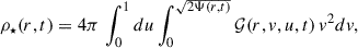
The initial velocity distribution was assumed to be isotropic, which allowed us to express the DF in terms of the original energy ε(t0) (Eq. [24]). However, the energy of a stellar orbit is not conserved during the expansion (![Mathematical equation: $ \varepsilon[t]\not= \varepsilon[t_0] $](/articles/aa/full_html/2025/10/aa55679-25/aa55679-25-eq35.gif) ) which, together with the conservation of the adiabatic invariants leads to final stellar orbits that are not isotropic. Following the arguments above, one can also compute the final velocity anisotropy parameter (Eq. (1)). Since the mean tangential and radial velocities are zero, the tangential and radial velocity dispersions are (e.g., Binney & Tremaine 2008)
) which, together with the conservation of the adiabatic invariants leads to final stellar orbits that are not isotropic. Following the arguments above, one can also compute the final velocity anisotropy parameter (Eq. (1)). Since the mean tangential and radial velocities are zero, the tangential and radial velocity dispersions are (e.g., Binney & Tremaine 2008)
 (35)
(35)
and
 (36)
(36)
which are formally identical to Eq. (18) except for the factors (v sin η)2 and (v cos η)2. Thus, the integration is identical to Eq. (33), except for these factors, leading to
 (37)
(37)
and
 (38)
(38)
The above equations are used in the next section to evaluate stellar density profiles and anisotropy parameters characteristic of stellar system with isotropic velocity distributions.
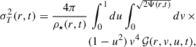
2.2.1. Examples of systems with initial isotropic orbits
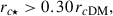
After setting the parameters that define the initial and the final DM profiles, Eqs. (1), (32), (33), (37), and (38) are used to evaluate the final stellar density profiles and the anisotropy parameters shown in Fig. 3. The single and double integrals in the equations were evaluated numerically at each radius r using the routine simpson from the Python package SciPy (Virtanen et al. 2020).
 |
Fig. 3. Simulations corresponding to an initially isotropic stellar distribution being hosted in a DM halo set by Henon’s isochrone potential. Each figure is split into two panels with the anisotropy parameter on top and the density profiles and core radii at the bottom. The color and line-type code for the densities (bottom panels) is the same as that used in Fig. 1 and 6. The inset in the top panel includes the actual value of β at the core radius rc of the final stellar distribution, as well as rc/2, 2 rc, and 3 rc. (a) The DM expands by a factor of 20. The polytropic index m is set to 5, and the cutoff radius of the initial stellar distribution to 1. The cutoff of the final stellar distribution is marked with a vertical dashed green line. (b) Same as (a) except for the initial cutoff, set to 1000. (c) Same as (a) except for the initial cutoff, set to 100, and the polytropic index, set to 2. (d) Same as (a) except for the DM expansion factor, which this time is about 350 (riso goes from 0.03 to 10). For reference, the four panels include an Osipkov-Merrit (OM) anisotropy distribution (the solid green lines), where β(r) = r2/(r2 + rOM2). In general, OM does a fair job when the characteristic radius, rOM, is tuned to a value much larger than the DM core radius. For further details on the types of line in the density sub-panels, see the caption of Fig. 1. |
The top panel within each sub-figure of Fig. 3 shows the anisotropy parameter of the final stellar distribution, whereas the bottom panel contains the relevant densities and core radii. By construction, the DM density creating the potential has a core whose size is set by riso and can be made small to represent initial conditions and large to represent the final ones (see the dashed and solid red lines in the bottom panels of Fig. 3). The DM cores are inherited by both the initial and the final stellar distributions (dashed blue lines and solid blue lines, respectively). We parameterize the expansion rate, for DM and for stars, as the ratio between the initial and final core radii defined in Eq. (15). The typical expansion rates of the stars are large but smaller than the expansion rate of the DM distribution that causes the stellar expansion. Stars expand about half the expansion of the DM, as it is registered in the inset of the different panels. The final stellar velocity anisotropy happens to be isotropic in the stellar core (β ≃ 0 for r ≲ rc) and becomes radially biased in the outskirts of the stellar profile (β ≳ 0 for r ≳ rc). Such radial anisotropy is never large within potentially observable radii. The shape resembles the Osipkov-Merrit anisotropy used in analytic studies, where β(r) = r2/(r2 + rOM2) with rOM a characteristic length scale; see the green curve in the top panels of Fig. 3.
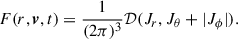
In order to quantify more precisely the velocity anisotropy produced by the DM expansion, we carried out a series of simulations where β is evaluated at different radii of the resulting stellar profile: at the core radius rc, within the core radius at rc/2, and outside the core at 2 rc and 3 rc radii. The results are condensed in Fig. 4, where β is represented against the free parameter that is varied in the simulation. We vary the polytropic index (2 ≤ m ≤ 6; the blue lines), the stellar cutoff radii (rcut, the orange lines), and the final DM core radius (riso, with rcut fixed to 1 and 100; the red and green lines, respectively). The simulations show that within the core β ≃ 0, with a typical value at rc around 0.07. Outside a core, β is positive and increases to typical values between 0.2 and 0.5.
 |
Fig. 4. Variation in the anisotropy parameter β at selected radii of the final stellar profile: at the core radius rc (the solid lines), within the core radius at rc/2 (the dotted lines) and outside the core at 2 rc and 3 rc radii (the dashed and dash-dotted lines, respectively). Different colors represent different varying parameter as indicated in the inset. The absolute variation, given in the inset, has been normalized so that if p is the varying parameter then the abscissa represents (p − minp)/(maxp − minp). The gravitational potential set by DM is an Henon’s isochrone with an initial stellar velocity distribution that is isotropic (Sect. 2.2). |
As far as the stellar density is concerned, the general behavior is summarized in Fig. 5. It shows the final core radius ratio ⋆ rc/DM rc (the solid lines), the final over initial core ratio of DM (the dashed lines), and the final over initial core ratio of the stars (the dotted lines). They are presented against the variation of the polytropic index (the blue lines), the cutoff radius of the initial stellar distribution (the orange lines), the initial core radius of DM (the green lines), and the initial core radius of DM but assuming circular orbits as worked out in Sect. 2.1 (the red lines). The main result is that the stellar expansion is smaller but of the same magnitude as that DM expansion driving it, and that the resulting stellar core is smaller but of similar size as the final DM core.
 |
Fig. 5. Ratio between radii characterizing the effect of the expansion of the DM halo on an initially isotropic stellar velocity distribution. It shows final core radius ratio ⋆ rc/DM rc (the solid lines), the final over initial core ratio of DM (the driving expansion rate, given by the dashed lines), and the final over initial core ratio of the stars (the resulting stellar expansion rate, given by the dotted lines). They are presented versus the variation of the polytropic index (the blue lines), the cutoff radius of the initial stellar distribution (the orange lines), the initial core radius of DM (the green lines), and the initial core radius of DM but assuming circular orbits (Sect. 2.1; the red lines). The gravitational potential is an Henon’s isochrone, and the varying parameter has been normalized as explained in the caption of Fig. 4. |
We argue in Appendix B that the expansion rate of the stars scales with the expansion rate of DM as a power law, with an exponent close to one (around 0.85; see Eq. (B.4)).
2.3. Radial stellar orbits in arbitrary spherical potentials
In stellar systems with radial orbits, the angular momentum is zero (L in Eq. (26)) since the radial vector and the velocity are defined to be parallel. Because the angular momentum is conserved during the assumed adiabatic expansion of the DM halo, the final stellar distribution also has radial orbits. Since L = 0, the dependence of both the initial and the final DF on L is through a Dirac δ+(L2) function (Fridman & Polyachenko 1984; Binney & Tremaine 2008, problem 4.9), explicitly,
![Mathematical equation: $$ \begin{aligned} F(r,\boldsymbol{v}) = \delta _+(L^2)\, \mathcal{F} ({\epsilon }) = \delta _+(L^2) \mathcal{F} [\Psi (r) - v^2/2]. \end{aligned} $$](/articles/aa/full_html/2025/10/aa55679-25/aa55679-25-eq40.gif) (39)
(39)
It follows directly from the above DF, by integrating over the velocities, that the spatial density is
![Mathematical equation: $$ \begin{aligned} \rho _\star (r) = \frac{2\pi }{r^2} \int _0^{\sqrt{2\Psi (r)}} dv\, \mathcal{F} [\Psi (r) - v^2/2]. \end{aligned} $$](/articles/aa/full_html/2025/10/aa55679-25/aa55679-25-eq41.gif) (40)
(40)
We then see that stellar systems with purely radial orbits do not admit stellar cores, since the density scales as ρ(r)∝r−2. These stellar systems are, however, rather artificial. Small perturbations lead to orbits that are not strictly radial that blur the central cusp.
For the purpose of illustration, we worked out the initial and final densities in a Henon’s potential (Eq. (16)), which allows for radial stellar orbits. In this case, Eq. (39) becomes,
![Mathematical equation: $$ \begin{aligned} F(r,\boldsymbol{v},t) = \delta _+(L^2)\,\mathcal{F} [\varepsilon (t_0)], \end{aligned} $$](/articles/aa/full_html/2025/10/aa55679-25/aa55679-25-eq42.gif) (41)
(41)
where we also assume a dependence of the DF on Jr identical to that used in Sect. 2.2. Inserting the DF, Eq. (41), into Eq. (18), one can show that the initial density is
![Mathematical equation: $$ \begin{aligned}&\rho _\star (r,t_0) = \frac{\pi \, 2^{3/2}}{r^2}\times \nonumber \\&\quad \left[\Psi (r,t_0)-\Psi (r_{cut},t_0)\right]^{m-1}\,\int ^1_0(1-x^2)^{m-3/2}dx, \end{aligned} $$](/articles/aa/full_html/2025/10/aa55679-25/aa55679-25-eq43.gif) (42)
(42)
whereas the final density is
 (43)
(43)
Setting u = 1 in 𝒢 (see the definition in Eq. (34)) corresponds to sin η = 0 and, consequently, to L = 0 (Eq. (26)).
Examples based on solving numerically Eqs. (42) and (43) are shown in Fig. 6. Contrarily to what happens with circular orbits (Fig. 1) and isotropic orbits (Fig. 3), the inner slope of the final stellar distribution never forms a core (the solid blue lines) despite the fact that the final DM profile has it (the solid red lines).
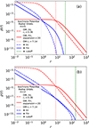 |
Fig. 6. Similar to Figs. 1 and 3, except that the orbits are radial, thus preventing the formation of a stellar core (see the solid blue lines, which behave as r−2 at small radii). The potential was assumed to be of the type Henon’s isochrone. (a) The DM expands a factor of 20, from riso = 0.5 to riso = 10. The polytropic index m is set to 5, and the cutoff radius of the initial stellar distribution to 10. The cutoff of the final stellar distribution is marked with a vertical dashed green line. (b) Same as (a) except for the initial cutoff, set to 100, and the polytropic index, set to 2. For further details, see the caption of Fig. 1. |
3. Initial conditions to be expected
As was described in Sect. 2, under quite general circumstances, the expansion of the DM halo forces the expansion of the initial stellar distribution that forms a core-like feature. However, the properties of the resulting stellar cores depend on the initial conditions of the distribution of DM and stars, including their relative size and the anisotropy of the stellar orbits. Thus, we address the question of which initial conditions can be expected, based on the existing literature. The result is discussed next and also summarized in Table 1.
Constraints on the expected initial and final conditions
Constraints on the initial DM distribution: According to the existing CDM numerical simulations, the first DM haloes have a power-law mass density distribution with the inner slope, cDM(t0), being around 1.5 or 2 (Tasitsiomi et al. 2004; Diemand et al. 2005; Yajima et al. 2017; Colombi 2021; Delos & White 2023a,b), which is significantly larger than the NFW slope (c = 1 in Eq. (9)). These high-redshift halos are also small, with typical concentrations (rs/rvir) around ∼5 independently of the DM halo mass (Anderhalden & Diemand 2013; Ishiyama 2014; Dutton & Macciò 2014; Correa et al. 2015; Sorini et al. 2025). The symbol rvir stands for the virial radius which depends on the total halo mass and the cosmological parameters so that, for the current cosmology and for halo mass from 106 to 108 M⊙, 0.3 < rvir < 1.3 kpc at redshift ten2 Thus, the typical initial scale radii, rs, span from 60 to 260 pc. These estimates are included in Table 1.
These conditions are derived from CDM simulations and, in principle, may not directly apply to other DM models where the expansion is significant (Sect. 1). However, the expansion we propose unfolds over long timescales, suggesting that the physical mechanism behind it is unlikely to play a major role until later epochs. At least, this is our working hypothesis so that the CDM initial conditions are assumed to hold for other types of DM.
Initial stellar distribution. There is no clear consensus in the literature regarding the stellar distribution that emerges as DM halos first form stars. In relatively massive objects going through major star formation episodes, the stellar surface density seems to be a power law at all times, with an exponent as negative as −2 (Lapiner et al. 2023). It remains to be determined how representative these starbursts are of star formation in smaller DM halos. As for the size, several recent numerical simulation impose stellar distributions with half-mass radius similar to the size of the DM distribution mentioned in the previous paragraph. For example, Ricotti et al. (2022) assume the stellar half-mass radius to DM virial radius of 0.15. With the typical concentrations of high-redshift DM halos (∼5), this ratio is equivalent to a ratio between stars and DM radii of ∼0.75, signaling their similarity. Ricotti et al. (2022) consider uncertainties exploring ratios in the range between 0.15 and 1.5. Querci et al. (2025) use initial (redshift 7) stellar distributions between 15 and 150 pc when the DM halo mass spans from 107.5 to 108 M⊙. Thus, the assumed initial stellar distribution is smaller but of the order of the rs defining the DM distribution. In short, the stellar distribution is likely a power law with negative exponent and a spatial extent smaller but not very different from the extent of the DM halos. These constraints agree with our argument in Appendix C that the half-mass radius of the initial stellar distribution has to be larger than 0.4 times the half-mass radius of the initial DM halo.
Another independent physical constraint on the original stellar distribution comes from the newborn star forming regions observed locally. We focus on large H II regions because they likely reflect the physical conditions characteristic of the early Universe, with abundant high-density gas ready to form stars. Thus, local analogs to high-redshift star formation could be the so-called super star clusters (SSC) observed to happen in, for example, major mergers of gas rich galaxies (Whitmore & Schweizer 1995). These SSCs are young (100 Myr), have stellar masses of around 105 M⊙ (Melo et al. 2005), and cored light distributions with half-light radii from a 3 to 10 pc (Cuevas-Otahola et al. 2020). Compared to the sizes of the initial DM distributions described above, these stellar radii represent a fraction going from approximately 0.1 to 1.5 times the DM radii. These estimates are included in Table 1.
Stellar velocity anisotropy: One of the conclusions reached in Sect. 2 is that an initial tangential or radial velocity anisotropy remains tangential or radial after the expansion. However, initially isotropic velocity distributions turn into isotropic in the formed core but radially biased beyond the core radius (Sect. 2.2 and Fig. 3). Thus, according to the DM expansion mechanism, the final anisotropy of the stellar velocity keeps memory of the initial conditions. Therefore, the question arises of what the observed anisotropy is. The velocity anisotropy observed in dwarf late type galaxies is quite uncertain and rely on modeling the velocity and mass distribution in dSph and UFDs. However, the consensus is that galaxies with cores have isotropic stellar velocities at the center (β ∼ 0; Łokas 2009, 2002; Zhu et al. 2016; Pascale et al. 2018; Kacharov et al. 2022; Kowalczyk & Łokas 2022). In order to be consistent with the proposed mechanism, the initial stellar velocity distribution should be close to isotropic. In the outskirts, outside the core, the observational situation is more complex with claims of observed tangential (Kowalczyk et al. 2019; Kacharov et al. 2022), radial (Pascale et al. 2018; Massari et al. 2020), or even mixed anisotropies depending on the axis of symmetry, the stellar component under study, or else (Zhu et al. 2016; Leung et al. 2021; Vitral et al. 2024).
A tendency to be isotropic in the center (β ∼ 0) and then radially biased (β > 0) is also found in cosmological CDM zoom-in simulations of the smallest galaxies (El-Badry et al. 2017; González-Samaniego et al. 2017; Orkney et al. 2023). The self-driven expansion of the DM halo is not expected to occur in these simulations and so the reason has to be other than the expansion. It is thought to be due to stellar feedback that produces episodic gas outflows, dropping the inner potential and placing stars on predominantly radial orbits (El-Badry et al. 2017). Although this sudden changes are irreversible and more effective, in a sense resemble the production of radial orbits described in Sect. 2.2. Galaxy mergers may also produce radial orbits (Orkney et al. 2023).
4. Discussion
The expected initial conditions described in Sect. 3 and Table 1 restrict the outcome of the mechanism in terms of the allowed stellar inner core-like structures, their extension and inner slope. The impact of these constraints is analyzed in the present section.
As we argue in Sect. 2, the physical process of DM expansion approximately conserves the anisotropy of the velocity distribution, at least in the innermost regions of the stellar profile. The observed dwarf galaxies seem to favor star with isotropic orbits in their center, therefore, using isotropy as initial conditions seems to be a reasonable guess. As is shown in Appendix B, even for initially isotropic orbits, the ratio between the final stellar and DM core sizes (rc⋆/rcDM) is approximately the same as the original one (rc0⋆/r0DM) except for a factor of order one (see Eq. (B.4)),
![Mathematical equation: $$ \begin{aligned} \frac{r_{c\star }}{r_{\mathrm{cDM}}} \simeq \frac{r_{c0\star }}{r_{0\mathrm{DM}}}\times \left[\frac{r_{\mathrm{c DM}}}{r_{0\mathrm{DM}}}\right]^{-0.15}. \end{aligned} $$](/articles/aa/full_html/2025/10/aa55679-25/aa55679-25-eq45.gif) (44)
(44)
When the DM expansion factor rcDM/r0DM varies from 5 to 15, the multiplying factor varies from 0.8 to 0.7. If we use the constraint that rc0⋆ > 0.4 r0DM (as worked out in Sect. 3 and Appendix C) then the expected initial conditions favor
 (45)
(45)
so that having rc⋆ ∼ rcDM or even rc⋆ > rcDM cannot be discarded.
The initial DM density is predicted to follow a power law with the exponent around −cDM(t0)∼ − 1.5 or a bit more negative. Since our study of the initial isotropic velocity distribution does not contemplate pure power law density profiles, we use here the constraint derived for circular orbits (Sect. 2.1). The stellar distribution is uncertain but is expected to be shallower than the DM, namely, c⋆(t0) < cDM(t0) (Table 1). This constraint, together with Eq. (11), implies the final stellar inner slope to be,
 (46)
(46)
where we have used the expected values for the initial and final DM slopes; cDM(t0) = 1.5 and cDM(t) = 0, respectively. Moreover, the stars will form perfect cores, c⋆(t) = 0, if the initial stellar slope is c⋆(t0)≃1 (see Eq. (12)).
5. Conclusions
Motivated by the observation of extended stellar cores, we explore a conceptually simple mechanism to form them in DM-dominated dwarf galaxies. A number of physical models of DM beyond CDM predict the thermalization of the DM distribution over time, which implies the expansion of an originally small cuspy DM halo to produce a core (see Sect. 1). This expansion reduces the gravitational force that holds the stars in the halo and drives its expansion to generate diffuse stellar system. Our analysis shows that this hypothetical mechanism works in practice.
We have studied three types of spherically symmetric systems with different velocity anisotropies covering all extremes, from purely tangential to purely radial orbits. Action adiabatic invariants allow us to study the behavior of a stellar distribution that evolves under the effects of a slowly changing potential, generated by a distribution of DM with an original cusp that turns into a core. We discuss the behavior under a broad range of initial and final conditions, finding that stellar cores are produced relatively easily. However, the properties of the induced stellar cores depend on these conditions. Thus, we reviewed the literature on the initial conditions expected from theoretical considerations, numerical simulations, and observational data, including the DM and stellar density profiles, as well as the stellar velocity anisotropy.
The main results of our analysis and the subsequent numerical solution of the relevant equations are:
– The conservation of the radial action variable implies that, for slowly changing central potentials, circular orbits (for which Jr = 0) remain circular. On the other hand, the conservation of angular momentum implies that purely radial orbits (for which L = 0) stay radial. Initially isotropic orbits remain approximately isotropic, at least in the central part of the stellar distribution (Sect. 2.2).
– When the orbits are circular (Sect. 2.1), initial DM NFW profiles produce stellar density profiles with core-like structure (i.e., c⋆[t]∼0) provided the initial stellar distribution has an inner slope (i.e., c⋆[t0]) in the range between 0.5 and 1.2. The stellar distribution can develop a central region lacking stars when they start off with an inner slope shallower than 0.5. The expansion rate of the stellar distribution scales with the expansion rate of the DM so that the process can also produce stellar cores smaller and larger than the DM cores depending on the initial conditions.
– The mechanism acting on purely radial orbits does not produce stellar cores because radial orbits evolve into radial orbits, and the density distribution of a system of radial orbits cannot have an inner core (Sect. 2.3).
– Initially isotropic orbits (Sect. 2.2) behave very much like circular orbits. The expansion induces cores with the expansion rate of the stars being similar to that of the DM driving the process. The formed cores remains isotropic but the expansion induces the development of radially biased orbits in the outskirts of the stellar distribution. Using β to parameterize the anisotropy (Eq. (1)), we find that it is approximately zero within the cores, with a typical value of around 0.07 at the core radius. Outside the core, β is positive and increases to typical values between 0.2 and 0.5 at 3 core radii (Figs. 3 and 4). It is qualitatively similar to the Osipkov-Merrit anisotropy.
– Given the sensitivity of the final stellar properties on the initial conditions of the DM and stars, we explore the literature for the expected conditions suggested by theory and observations (Sect. 3). Table 1 summarizes them. The initial density of the DM halos follows a power law of large negative slope (∼ − 1.5). The initial stellar distribution is expected to be shallower than this, but with a size similar to the DM distribution (see also Appendix C). Although the stellar velocities observed in the local universe are very uncertain, the centers of the dwarf galaxies tend to be isotropic. Isotropy is likely the initial condition too provided the expansion mechanism work since it tends to conserve the type of anisotropy of the velocity distribution.
– Given the properties of the stellar distribution after expansion (Sect. 2) and the expected initial conditions (Table 1), the stellar distribution is likely to form a core-like structure of size rc⋆ > 0.30 rcDM, with rcDM the DM core of the final distribution. Thus, stellar cores with the size of the DM distribution or even larger can be produced by the mechanism. In addition, the final inner slope c⋆(t) has to be smaller than ∼0.6. Perfect stellar cores are formed if the initial stellar slope was c⋆(t0)≃1.
We have restricted this study to analytical models, enough to provide physical insight, simple to deal with, but difficult to compare with actual observations. Numerical modeling is needed to treat lack of spherical symmetry or to include the existence of several stellar component formed in different times and with different kinematic properties (Battaglia et al. 2008; Pace et al. 2020; Tolstoy et al. 2023). Numerical modeling is also needed to include the self-gravity of the stars, which has been neglected in our analysis. It is a good approximation for some interesting objects (e.g., Sánchez Almeida et al. 2024b), but not in general. Often baryons contribute significantly to the inner potential and then DM cores can be produced by stellar feedback (Governato et al. 2010; Pontzen & Governato 2012). A fully self-consistent treatment of DM and baryons is technically very challenging, but one can reasonably adopt the rule of thumb used in the CDM framework: stellar feedback is unable to modify the DM halo in galaxies with stellar mass below 105–106 M⊙ (e.g., Peñarrubia et al. 2012). Moreover, some useful simulations exist already. We note the existence of cosmological numerical simulation of galaxy formation that considers the DM to be self-interacting so that the DM halos develop inner cores over time driven by DM – DM particle collisions (SIDM; e.g., Elbert et al. 2015; Outmezguine et al. 2023; Correa et al. 2025). In these simulations, the stars form cores that trace the evolution of the SIDM halos, in line with what we find. In particular, the size of the formed stellar cores is closely related to the size of the DM cores (e.g. Vogelsberger et al. 2014; Zhang et al. 2024).
Ultimately, we would like to compare the predictions of the mechanism with observed properties of stellar cores in dwarf galaxies – for example, the stellar and DM core radii, and their dependence on stellar and DM masses. This comparison requires setting up cosmological numerical simulations with various flavors of DM that take self-consistently into account the baryon driven processes that reshape the distribution of DM and stars. While such a direct comparison remains out of reach, the slow expansion mechanism can, in principle, generate stellar cores of any size in galaxies of arbitrary mass, given suitable initial conditions and DM halo expansions. In the real galaxies, differences in initial conditions and star-formation histories are to be expected. Moreover, the DM expansion factors may be very different for halos of similar mass (e.g., in SIDM, subtle differences determine whether a particular halo expands, and so ends up with a large core, or core-collapses, and then produces a small one – see Kahlhoefer et al. 2019; Nadler et al. 2023). The mechanism likely renders a diversity of stellar cores and, in this broad sense, is consistent with observations.
It is an abc profile with a, b, c = 2, 5, 0.
For the current cosmology, with Ωm = 0.3 and ΩΛ = 0.7, rvir ≃ 9.6 kpc [MDM(< rvir)/108 M⊙]1/3 [0.7 + 0.3 (1 + z)3]−1/3, with z the redshift and MDM(< rvir) the DM halo mass within the virial radius (e.g., see Querci et al. 2025).
Following the notation in Sect. 2.1.1, cDM should formally be written as cDM(t0). However, for the sake of brevity, we omit the explicit t0 dependence for this and other variables throughout this appendix, without any loss of clarity.
Acknowledgments
Thanks are due to Claudio Dalla Vecchia for insightful discussions on various issues addressed in the manuscript, and to Giuseppina Battaglia for comments and references on the observed β. We also thank the anonymous referee for comments that helped clarify the arguments. The research of JSA is partly funded through grant PID2022-136598NB-C31 (ESTALLIDOS 8) by the Spanish Ministry of Science and Innovation (MCIN/AEI/10.13039/501100011033) and “ERDF A way of making Europe”. The three authors have been supported by the European Union through the grant “UNDARK” of the Widening participation and spreading excellence programe (project number 101159929). IT acknowledges support from the ACIISI, Consejería de Economía, Conocimiento y Empleo del Gobierno de Canarias and the European Regional Development Fund (ERDF) under a grant with reference PROID2021010044 and from the State Research Agency (AEI-MCINN) of the Spanish Ministry of Science and Innovation under the grant PID2022-140869NB-I00 and IAC project P/302302, financed by the Ministry of Science and Innovation, through the State Budget and by the Canary Islands Department of Economy, Knowledge, and Employment, through the Regional Budget of the Autonomous Community. He also acknowledges support from the European Union through the grant “Excellence in Galaxies – Twinning the IAC” of the EU Horizon Europe Widening Actions programmes (project numbers 101158446). Funding for this research was provided by the European Union (MSCA EDUCADO, GA 101119830). Views and opinions expressed are however those of the author only and do not necessarily reflect those of the European Union or European Research Executive Agency (REA). Neither the European Union nor the granting authority can be held responsible for them.
References
- Anderhalden, D., & Diemand, J. 2013, JCAP, 2013, 009 [Google Scholar]
- Argüelles, C. R., Becerra-Vergara, E. A., Rueda, J. A., & Ruffini, R. 2023, Universe, 9, 197 [CrossRef] [Google Scholar]
- Arias, J. M., Bell, E. F., Gozman, K., et al. 2025, ApJ, 982, L3 [Google Scholar]
- Battaglia, G., Helmi, A., Tolstoy, E., et al. 2008, ApJ, 681, L13 [NASA ADS] [CrossRef] [Google Scholar]
- Binggeli, B., Sandage, A., & Tarenghi, M. 1984, AJ, 89, 64 [NASA ADS] [CrossRef] [Google Scholar]
- Binney, J., & Tremaine, S. 2008, Galactic Dynamics, 2nd edn. (Princeton: Princeton University Press) [Google Scholar]
- Blumenthal, G. R., Faber, S. M., Flores, R., & Primack, J. R. 1986, ApJ, 301, 27 [Google Scholar]
- Bode, P., Ostriker, J. P., & Turok, N. 2001, ApJ, 556, 93 [Google Scholar]
- Caldwell, N., & Bothun, G. D. 1987, AJ, 94, 1126 [Google Scholar]
- Campbell, D. J. R., Frenk, C. S., Jenkins, A., et al. 2017, MNRAS, 469, 2335 [Google Scholar]
- Carlsten, S. G., Greene, J. E., Beaton, R. L., Danieli, S., & Greco, J. P. 2022, ApJ, 933, 47 [CrossRef] [Google Scholar]
- Chu, X., & Garcia-Cely, C. 2018, JCAP, 2018, 013 [Google Scholar]
- Colín, P., Avila-Reese, V., & Valenzuela, O. 2000, ApJ, 542, 622 [NASA ADS] [CrossRef] [Google Scholar]
- Colombi, S. 2021, A&A, 647, A66 [NASA ADS] [CrossRef] [EDP Sciences] [Google Scholar]
- Conselice, C. J. 2018, Res. Notes Am. Astron. Soc., 2, 43 [Google Scholar]
- Correa, C. A., Schaller, M., Schaye, J., et al. 2025, MNRAS, 536, 3338 [Google Scholar]
- Correa, C. A., Wyithe, J. S. B., Schaye, J., & Duffy, A. R. 2015, MNRAS, 452, 1217 [CrossRef] [Google Scholar]
- Cuevas-Otahola, B., Mayya, Y. D., Puerari, I., & Rosa-González, D. 2020, MNRAS, 492, 993 [NASA ADS] [CrossRef] [Google Scholar]
- Delgado, V., & Muñoz Mateo, A. 2023, MNRAS, 518, 4064 [Google Scholar]
- Delos, M. S., & White, S. D. M. 2023a, MNRAS, 518, 3509 [Google Scholar]
- Delos, M. S., & White, S. D. M. 2023b, JCAP, 2023, 008 [CrossRef] [Google Scholar]
- Di Cintio, A., Brook, C. B., Dutton, A. A., et al. 2017, MNRAS, 466, L1 [NASA ADS] [CrossRef] [Google Scholar]
- Diemand, J., Moore, B., & Stadel, J. 2005, Nature, 433, 389 [Google Scholar]
- Dutton, A. A., & Macciò, A. V. 2014, MNRAS, 441, 3359 [Google Scholar]
- El-Badry, K., Wetzel, A. R., Geha, M., et al. 2017, ApJ, 835, 193 [NASA ADS] [CrossRef] [Google Scholar]
- Elbert, O. D., Bullock, J. S., Garrison-Kimmel, S., et al. 2015, MNRAS, 453, 29 [NASA ADS] [CrossRef] [Google Scholar]
- Fridman, A. M., & Polyachenko, V. L. 1984, Physics of Gravitating Systems. I. Equilibrium and Stability [Google Scholar]
- Gnedin, O. Y., Kravtsov, A. V., Klypin, A. A., & Nagai, D. 2004, ApJ, 616, 16 [Google Scholar]
- González-Samaniego, A., Bullock, J. S., Boylan-Kolchin, M., et al. 2017, MNRAS, 472, 4786 [CrossRef] [Google Scholar]
- Governato, F., Brook, C., Mayer, L., et al. 2010, Nature, 463, 203 [NASA ADS] [CrossRef] [Google Scholar]
- Henon, M. 1959a, Ann. d’Astrophys., 22, 491 [Google Scholar]
- Henon, M. 1959b, Ann. d’Astrophys., 22, 126 [Google Scholar]
- Hénon, M. 1960, Ann. d’Astrophys., 23, 474 [Google Scholar]
- Hernquist, L. 1990, ApJ, 356, 359 [Google Scholar]
- Indjin, M., Liu, I. K., Proukakis, N. P., & Rigopoulos, G. 2025, ArXiv e-prints [arXiv:2502.04838] [Google Scholar]
- Ishiyama, T. 2014, ApJ, 788, 27 [Google Scholar]
- Kacharov, N., Alfaro-Cuello, M., Neumayer, N., et al. 2022, ApJ, 939, 118 [NASA ADS] [CrossRef] [Google Scholar]
- Kahlhoefer, F., Kaplinghat, M., Slatyer, T. R., & Wu, C.-L. 2019, JCAP, 2019, 010 [CrossRef] [Google Scholar]
- Kowalczyk, K., & Łokas, E. L. 2022, A&A, 659, A119 [NASA ADS] [CrossRef] [EDP Sciences] [Google Scholar]
- Kowalczyk, K., del Pino, A., Łokas, E. L., & Valluri, M. 2019, MNRAS, 482, 5241 [NASA ADS] [CrossRef] [Google Scholar]
- Lapiner, S., Dekel, A., Freundlich, J., et al. 2023, MNRAS, 522, 4515 [NASA ADS] [CrossRef] [Google Scholar]
- Lazar, A., Bullock, J. S., Boylan-Kolchin, M., et al. 2020, MNRAS, 497, 2393 [NASA ADS] [CrossRef] [Google Scholar]
- Leung, G. Y. C., Leaman, R., Battaglia, G., et al. 2021, MNRAS, 500, 410 [Google Scholar]
- Łokas, E. L. 2002, MNRAS, 333, 697 [CrossRef] [Google Scholar]
- Łokas, E. L. 2009, MNRAS, 394, L102 [NASA ADS] [CrossRef] [Google Scholar]
- Massari, D., Helmi, A., Mucciarelli, A., et al. 2020, A&A, 633, A36 [NASA ADS] [CrossRef] [EDP Sciences] [Google Scholar]
- Melo, V. P., Muñoz-Tuñón, C., Maíz-Apellániz, J., & Tenorio-Tagle, G. 2005, ApJ, 619, 270 [Google Scholar]
- Merritt, D., Graham, A. W., Moore, B., Diemand, J., & Terzić, B. 2006, AJ, 132, 2685 [Google Scholar]
- Mihos, J. C., Durrell, P. R., Ferrarese, L., et al. 2015, ApJ, 809, L21 [Google Scholar]
- Mocz, P., Vogelsberger, M., Robles, V. H., et al. 2017, MNRAS, 471, 4559 [Google Scholar]
- Montes, M., Trujillo, I., Karunakaran, A., et al. 2024, A&A, 681, A15 [NASA ADS] [CrossRef] [EDP Sciences] [Google Scholar]
- Müller, O., Jerjen, H., & Binggeli, B. 2018, A&A, 615, A105 [Google Scholar]
- Nadler, E. O., Yang, D., & Yu, H.-B. 2023, ApJ, 958, L39 [NASA ADS] [CrossRef] [Google Scholar]
- Navarro, J. F., Frenk, C. S., & White, S. D. M. 1997, ApJ, 490, 493 [Google Scholar]
- Orkney, M. D. A., Taylor, E., Read, J. I., et al. 2023, MNRAS, 525, 3516 [NASA ADS] [CrossRef] [Google Scholar]
- Outmezguine, N. J., Boddy, K. K., Gad-Nasr, S., Kaplinghat, M., & Sagunski, L. 2023, MNRAS, 523, 4786 [NASA ADS] [CrossRef] [Google Scholar]
- Pace, A. B., Kaplinghat, M., Kirby, E., et al. 2020, MNRAS, 495, 3022 [NASA ADS] [CrossRef] [Google Scholar]
- Pascale, R., Posti, L., Nipoti, C., & Binney, J. 2018, MNRAS, 480, 927 [Google Scholar]
- Peñarrubia, J., Pontzen, A., Walker, M. G., & Koposov, S. E. 2012, ApJ, 759, L42 [CrossRef] [Google Scholar]
- Planck Collaboration XIII 2016, A&A, 594, A13 [NASA ADS] [CrossRef] [EDP Sciences] [Google Scholar]
- Plastino, A. R., & Plastino, A. 1993, Phys. Lett. A, 174, 384 [NASA ADS] [CrossRef] [Google Scholar]
- Pontzen, A., & Governato, F. 2012, MNRAS, 421, 3464 [NASA ADS] [CrossRef] [Google Scholar]
- Querci, L., Pallottini, A., Branca, L., & Salvadori, S. 2025, A&A, 694, A17 [NASA ADS] [CrossRef] [EDP Sciences] [Google Scholar]
- Richstein, H., Kallivayalil, N., Simon, J. D., et al. 2024, ApJ, 967, 72 [NASA ADS] [CrossRef] [Google Scholar]
- Ricotti, M., Polisensky, E., & Cleland, E. 2022, MNRAS, 515, 302 [CrossRef] [Google Scholar]
- Robertson, A., Massey, R., Eke, V., Schaye, J., & Theuns, T. 2021, MNRAS, 501, 4610 [NASA ADS] [CrossRef] [Google Scholar]
- Román, J., & Trujillo, I. 2017, MNRAS, 468, 4039 [Google Scholar]
- Saha, P. 1991, MNRAS, 248, 494 [NASA ADS] [CrossRef] [Google Scholar]
- Sánchez Almeida, J. 2025, Galaxies, 13, 6 [Google Scholar]
- Sánchez Almeida, J., & Trujillo, I. 2021, MNRAS, 504, 2832 [CrossRef] [Google Scholar]
- Sánchez Almeida, J., Trujillo, I., & Plastino, A. R. 2020, A&A, 642, L14 [NASA ADS] [CrossRef] [EDP Sciences] [Google Scholar]
- Sánchez Almeida, J., Plastino, A. R., & Trujillo, I. 2024a, A&A, 690, A151 [NASA ADS] [CrossRef] [EDP Sciences] [Google Scholar]
- Sánchez Almeida, J., Trujillo, I., & Plastino, A. R. 2024b, ApJ, 973, L15 [Google Scholar]
- Sánchez Almeida, J., Trujillo, I., Montes, M., & Plastino, A. R. 2025, A&A, 694, A283 [NASA ADS] [CrossRef] [EDP Sciences] [Google Scholar]
- Schive, H.-Y., Chiueh, T., & Broadhurst, T. 2014, Nat. Phys., 10, 496 [NASA ADS] [CrossRef] [Google Scholar]
- Simon, J. D. 2019, ARA&A, 57, 375 [NASA ADS] [CrossRef] [Google Scholar]
- Sorini, D., Bose, S., Pakmor, R., et al. 2025, MNRAS, 536, 728 [Google Scholar]
- Spergel, D. N., & Steinhardt, P. J. 2000, Phys. Rev. Lett., 84, 3760 [NASA ADS] [CrossRef] [Google Scholar]
- Tasitsiomi, A., Kravtsov, A. V., Gottlöber, S., & Klypin, A. A. 2004, ApJ, 607, 125 [NASA ADS] [CrossRef] [Google Scholar]
- Tolstoy, E., Skúladóttir, Á., Battaglia, G., et al. 2023, A&A, 675, A49 [NASA ADS] [CrossRef] [EDP Sciences] [Google Scholar]
- Trujillo, I. 2021, Nat. Astron., 5, 1182 [Google Scholar]
- van Dokkum, P. G., Abraham, R., Merritt, A., et al. 2015, ApJ, 798, L45 [NASA ADS] [CrossRef] [Google Scholar]
- Virtanen, P., Gommers, R., Oliphant, T. E., et al. 2020, Nat. Methods, 17, 261 [Google Scholar]
- Vitral, E., van der Marel, R. P., Sohn, S. T., et al. 2024, ApJ, 970, 1 [Google Scholar]
- Vogelsberger, M., Zavala, J., Simpson, C., & Jenkins, A. 2014, MNRAS, 444, 3684 [CrossRef] [Google Scholar]
- Whitmore, B. C., & Schweizer, F. 1995, AJ, 109, 960 [NASA ADS] [CrossRef] [Google Scholar]
- Yajima, H., Nagamine, K., Zhu, Q., Khochfar, S., & Dalla Vecchia, C. 2017, ApJ, 846, 30 [Google Scholar]
- Zhang, X., Yu, H.-B., Yang, D., & An, H. 2024, ApJ, 968, L13 [NASA ADS] [CrossRef] [Google Scholar]
- Zhu, L., van de Ven, G., Watkins, L. L., & Posti, L. 2016, MNRAS, 463, 1117 [Google Scholar]
Appendix A: General central potentials
In the main text, we treat circular, isotropic, and radial stellar orbits as separate cases. Nevertheless, the method is versatile and can be applied to general central potentials with any anisotropy, as outlined in here.
Let us consider a general central potential, Φ(r, p), which depends on one or more parameters collectively denoted by p. Because of the spherical symmetry assumption, the three action variables are Jr, Jθ = L − |Lz|, and Jϕ = Lz (e.g., Binney & Tremaine 2008, Sect. 3.5.2). There is no closed analytical expression for the action Jr, which has to be evaluated numerically. For an orbit of a particle moving in the potential Φ(r, p) with total energy E, the action Jr is given by the integral
![Mathematical equation: $$ \begin{aligned} J_r = \frac{1}{\pi } \int _{r_{min}}^{r_{max}} \, dr \, \sqrt{2 \Big [ E-\Phi (r,p) \Bigr ] - \frac{L^2}{r^2}}, \end{aligned} $$](/articles/aa/full_html/2025/10/aa55679-25/aa55679-25-eq48.gif) (A.1)
(A.1)
where
rmax and rmin are the two roots of
![Mathematical equation: $$ \begin{aligned} 2 \Bigl [E-\Phi (r,b) \Bigl ] - \frac{L^2}{r^2} \, = \, 0. \end{aligned} $$](/articles/aa/full_html/2025/10/aa55679-25/aa55679-25-eq49.gif) (A.2)
(A.2)
To study the behavior of the stellar distribution when the potential changes slowly, one has first to choose a distribution in action space defined through the action variables,
 (A.3)
(A.3)
The distribution in action space stays invariant during the slow evolution of the potential from an initial potential given by parameters p(t0) to a final one given by parameters p(t). To evaluate the initial phase-space density in a point (r, v), one first computes E and L. We note that the distribution depends only on the radial coordinate r, but depends on the full vector velocity, v, so that there is no restriction on its anisotropy. Then, though the numerical evaluation of the integral in Eq. (A.1), using the initial parameters p(t0), one computes Jr as a function of r and v. Then, keeping in mind that
 (A.4)
(A.4)
one evaluates 𝒟(Jr, Jθ + |Jϕ|). This procedure gives the value of 𝒟 at any point (r, v). Once 𝒟(Jr, Jθ + |Jϕ|) is known, one evaluates numerically the two-dimensional definite integral required to determine the initial mass density profile (Eq. [18]),
![Mathematical equation: $$ \begin{aligned} \rho _{\star }(r,t_0) = 4\pi \int _0^1 du \int _0^{\sqrt{2\Psi (r,t_0)}} dv \, v^2 \,\times \nonumber \\ \mathcal{D} \left( J_r\left[ E = E(t_0), L = rv \sqrt{1-u^2}, p = p(t_0) \right], L = rv \sqrt{1-u^2} \right), \\ \end{aligned} $$](/articles/aa/full_html/2025/10/aa55679-25/aa55679-25-eq52.gif) (A.5)
(A.5)
where
and
![Mathematical equation: $$ \begin{aligned} \Psi (r,t) =-\Phi [r,p(t)]. \end{aligned} $$](/articles/aa/full_html/2025/10/aa55679-25/aa55679-25-eq54.gif)
To clarify the meaning of the above equation, a few comments are in order. One regards Jr as a function of u, and v through E = E(t0) and  . So does 𝒟, which depends on L in two ways, explicitly, and though Jr. The same procedure is used to evaluate the final density profile ρ⋆(r, t), with the same 𝒟(Jr, Jθ + |Jϕ|) but using the set of parameters p(t) corresponding to the final potential. That is,
![Mathematical equation: $$ \begin{aligned} \rho _{\star }(r,t) = 4\pi \int _0^1 du \int _0^{\sqrt{2\Psi (r,t)}} dv \, v^2 \,\times \nonumber \\ \mathcal{D} \left( J_r\left[ E = E(t), L = rv \sqrt{1-u^2}, p = p(t) \right], L = rv \sqrt{1-u^2} \right). \end{aligned} $$](/articles/aa/full_html/2025/10/aa55679-25/aa55679-25-eq56.gif) (A.6)
(A.6)
Appendix B: Does the final stellar core trace the underlying DM core?
The short answer to the question in the title of this appendix is “only when the original DM and stellar distributions have similar sizes”. The expansion in DM and stars is expected to be similar. The argument goes as follows. Considering circular orbits, the expansion of the stars following the DM core formation is controlled by Eq. (6). If a perfect DM core is formed, then the final DM density in the core is equal to
where rcDM is the DM core radius and we have assumed that the mass internal to the final DM core radius has not changed much during the expansion so that

Moreover, because of the existence of the central core,
Using these expressions, Eq. (6) can be re-written as,
![Mathematical equation: $$ \begin{aligned} \frac{r_{c\star }}{r_{c\mathrm{DM}}}=\left(\frac{r_{c0\star }}{r_{c\mathrm{DM}}}\right)^{1/4} \left[\frac{M_{\rm DM}(<r_{c0\star },t_0)}{M_{\rm DM}( < r_{c\mathrm{DM}},t_0)}\right]^{1/4} , \end{aligned} $$](/articles/aa/full_html/2025/10/aa55679-25/aa55679-25-eq60.gif) (B.1)
(B.1)
with rc0⋆ the original radius of the stars that end at the final stellar core radius rc⋆. Assuming that the original DM distribution has a characteristic density with a size r0DM, then
 (B.2)
(B.2)
which allows us to re-write Eq. (B.1) as
![Mathematical equation: $$ \begin{aligned} \frac{r_{c\star }}{r_{c0\star }} \simeq \left[\frac{r_{c\mathrm{DM}}}{r_{0\mathrm{DM}}}\right]^{3/4} . \end{aligned} $$](/articles/aa/full_html/2025/10/aa55679-25/aa55679-25-eq62.gif) (B.3)
(B.3)
Equation (B.3) tells that the expansion rate of the DM ∼rcDM/r0DM, is similar to the expansion rate produced on the stars, rc⋆/rc0⋆. Thus, if the sizes of the original stellar and DM distribution are similar, the resulting cores are similar too. However, the process can also produce stellar cores smaller and larger than the DM cores. It all depends on the original ratio between the stellar and DM distributions. This dependence can be seen in Fig. 2, top panel; compare the final axial ratio with original sizes parameterized by rs⋆/rsDM.
The above derivation assumes circular stellar orbits, but it also holds approximately for the isotropic velocities worked out in Sect. 2.2. The symbols in Fig. B.1 show a scatter plot of rc⋆/rc0⋆ versus rcDM/r0DM for the various types of potentials and expansions considered in Figs. 4 and 5. The stellar expansion ratio rc⋆/rc0⋆ approximately scales with the DM expansion ratio rcDM/r0DM driving the evolution. As the solid red line in Fig. B.1 shows, the expansion is approximately given by
![Mathematical equation: $$ \begin{aligned} \frac{r_{c\star }}{r_{c0\star }} \simeq \left[\frac{r_{c\mathrm{DM}}}{r_{0\mathrm{DM}}}\right]^{0.85} . \end{aligned} $$](/articles/aa/full_html/2025/10/aa55679-25/aa55679-25-eq63.gif) (B.4)
(B.4)
with the exponent in between 0.75 (as in Eq. [B.3], represented by the dashed blue line) and 0.95 (the dashed green line).
 |
Fig. B.1. Scatter plot of stellar expansion rate, rc⋆/rc0⋆, versus the DM expansion rate, rcDM/r0DM, for the various types of isotropic velocity distributions analyzed in Figs. 4 and 5. The color code of the symbols and the labels are inherited from these two previous figures. The relationship is approximately a power law of exponent 0.85 (the solid red line). Two other exponents are shown for reference; in particular, 0.75 represents the scaling derived for circular orbits and given in Eq. (B.3). |
Appendix C: Size of the initial stellar distribution relative to the DM
As discussed in Sect. 3, the first DM halos have a power law density distribution,
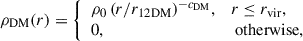 (C.1)
(C.1)
with r12DM the half-mass radius and ρ0 = ρDM(r12DM). Independently of the halo mass (and so of the virial radius rvir), the exponent3cDM is expected to be in the range 1.5 – 2. Keeping in mind that the total mass up to a radius r (< rvir) given by Eq. (C.1) is
![Mathematical equation: $$ \begin{aligned} M_{\rm DM}( < r) = \frac{4\pi \rho _0\,r_{12\mathrm{DM}}^3}{3-c_{\rm DM}}\left[\frac{r}{r_{12\mathrm{DM}}}\right]^{3-c_{\rm DM}}, \end{aligned} $$](/articles/aa/full_html/2025/10/aa55679-25/aa55679-25-eq65.gif) (C.2)
(C.2)
then the half-mass radius satisfies
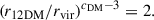 (C.3)
(C.3)
The DM halos forming stars for the first time collapse from material having the cosmic baryon fraction, fb ≃ 0.16 (e.g., Planck Collaboration XIII 2016). The baryons arrive as gas from which stars form and from which stars inherit proper motions and spatial distribution. As the gas radiates energy away, it cools and tends to sink toward the center of the gravitational potential, leading to a partial segregation from the DM. The gas also experiences hydrodynamical forces, which help reaching thermodynamic equilibrium and forming a core-like feature in the central region of its distribution (e.g., Binney & Tremaine 2008). For the sake of finding simple mathematical relations, this centrally concentrated cored gas distribution is approximated here as a top-hat function of half-mass radius r12g,
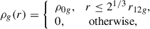 (C.4)
(C.4)
but more general gas distributions are used below. The total DM mass for the density in Eq. (C.1) is
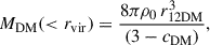 (C.5)
(C.5)
whereas the mass of the gas from Eq. (C.4) is
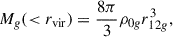 (C.6)
(C.6)
provided 21/3 r12g < rvir. Pieced together, the two previous equations lead to
![Mathematical equation: $$ \begin{aligned} \frac{M_g(<r_{\rm vir})}{M_{\rm DM}( < r_{\rm vir})}=\frac{f_b}{1-f_b} = (1-c_{\rm DM}/3)\left[\frac{r_{12g}}{r_{12\mathrm{DM}}}\right]^3\frac{\rho _{0g}}{\rho _0}. \end{aligned} $$](/articles/aa/full_html/2025/10/aa55679-25/aa55679-25-eq70.gif) (C.7)
(C.7)
If we ask the DM to be more important than the gas at all radii, as expected in DM dominated systems, this imposes
![Mathematical equation: $$ \begin{aligned} \rho _{0g} < \rho _0\,\left[\frac{2^{1/3}\,r_{12g}}{r_{12\mathrm{DM}}}\right]^{-c_{\rm DM}}, \end{aligned} $$](/articles/aa/full_html/2025/10/aa55679-25/aa55679-25-eq71.gif) (C.8)
(C.8)
which, together with Eqs. Eq. (C.3) and (C.7), lead to a lower limit for the gas half-mass radius,
![Mathematical equation: $$ \begin{aligned} r_{12g}> r_{12\mathrm{DM}}\,\left[\frac{f_b}{1-f_b}\frac{2^{c_{\rm DM}/3}}{(1-c_{\rm DM}/3)}\right]^{1/(3-c_{\rm DM})}. \end{aligned} $$](/articles/aa/full_html/2025/10/aa55679-25/aa55679-25-eq72.gif) (C.9)
(C.9)
Using typical values for the two relevant parameters (fb = 0.16 and cDM = 1.5), one gets
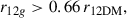 (C.10)
a limit pretty insensitive to variation of the parameters within expected boundaries.
The limit in Eq. (C.10) is similar to those found when, rather than a top-hat function, smooth more realistic functions are used to represent ρg(r). For example, for a NFW profile (Eq. [9], with a, b, c = 2, 3, 1) one finds r12g > 0.55 r12DM, for a Schuster-Plummer profile (Eq. [9], with a, b, c = 2, 5, 0) one finds r12g > 0.39 r12DM, and for a profile with a inner slope different form zero (Eq. [9], with a, b, c = 2, 20, 0.5) one finds r12g > 0.37 r12DM. Figure C.1 shows the functions used in the third example. The above values have been found numerically using Eqs. (C.3), (C.5), and (C.7), and then determining the smallest r12g which stills allows ρDM(r) > ρg(r) for all r.
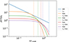 |
Fig. C.1. Example of the DM and gas densities used to represent the initial DM halos. For the DM to dominate at all radii, the sizes of the DM and gas distributions have to be comparable. The power-law DM density profile is shown as the solid blue line, with the virial radius marked as a vertical dashed blue line. The gas profiles are shown in different colors with the half-mass radii shown as vertical dotted lines with the color corresponding to the gas profile. Radii are normalized to the half mass radius of the DM distribution r12DM. The half-mass radii of the gas distribution has to be larger than 0.37 times the half-mass radius for the DM density to be larger than the gas density. The solid orange line shows this limiting case. |
In short, if the initial stellar distribution inherits its extent from the gas distribution from which it was born, then the extent of the stars and the extent of DM are expected to be similar (Eq. [C.10]).
All Tables
All Figures
|
Fig. 1. Examples of the impact of the DM core formation (from the initial dashed red lines to the final solid red lines) on the formation of a stellar core (the solid blue lines) evolving from an originally concentrated stellar distribution (the dashed blue lines). The vertical dotted lines indicate the radius of the formed cores in DM (red) and stars (blue). The initial stars are assumed to follow circular orbits. For details on the types of profiles represented in the different panels, see Sect. 2.1.2. Arbitrary global scale factors affect both densities and radii. |
| In the text | |
|
Fig. 2. Summary of the effect of the DM halo expansion on the stellar distribution when the orbits are circular (β = −∞). Two parameters are used to characterize the result: the ratio between the stellar and DM cores (top panel) and the final inner slope of the resulting stellar profile (bottom panel). Both are represented against the initial inner slope of the stellar distribution. The inset next to the top panel describes the initial and final DM profiles, with a, b, cDM referring to the parameters defining the ρabc profiles in Eq. (9). The solid black line labeled “Theory” in the bottom panel represents Eq. (11). The vertical dashed lines mark the initial cDM and follows the same color code as the upper panel. For further details, see Sect. 2.1.2. The region shaded in gray represents the approximate location of an observed stellar core. |
| In the text | |
|
Fig. 3. Simulations corresponding to an initially isotropic stellar distribution being hosted in a DM halo set by Henon’s isochrone potential. Each figure is split into two panels with the anisotropy parameter on top and the density profiles and core radii at the bottom. The color and line-type code for the densities (bottom panels) is the same as that used in Fig. 1 and 6. The inset in the top panel includes the actual value of β at the core radius rc of the final stellar distribution, as well as rc/2, 2 rc, and 3 rc. (a) The DM expands by a factor of 20. The polytropic index m is set to 5, and the cutoff radius of the initial stellar distribution to 1. The cutoff of the final stellar distribution is marked with a vertical dashed green line. (b) Same as (a) except for the initial cutoff, set to 1000. (c) Same as (a) except for the initial cutoff, set to 100, and the polytropic index, set to 2. (d) Same as (a) except for the DM expansion factor, which this time is about 350 (riso goes from 0.03 to 10). For reference, the four panels include an Osipkov-Merrit (OM) anisotropy distribution (the solid green lines), where β(r) = r2/(r2 + rOM2). In general, OM does a fair job when the characteristic radius, rOM, is tuned to a value much larger than the DM core radius. For further details on the types of line in the density sub-panels, see the caption of Fig. 1. |
| In the text | |
|
Fig. 4. Variation in the anisotropy parameter β at selected radii of the final stellar profile: at the core radius rc (the solid lines), within the core radius at rc/2 (the dotted lines) and outside the core at 2 rc and 3 rc radii (the dashed and dash-dotted lines, respectively). Different colors represent different varying parameter as indicated in the inset. The absolute variation, given in the inset, has been normalized so that if p is the varying parameter then the abscissa represents (p − minp)/(maxp − minp). The gravitational potential set by DM is an Henon’s isochrone with an initial stellar velocity distribution that is isotropic (Sect. 2.2). |
| In the text | |
|
Fig. 5. Ratio between radii characterizing the effect of the expansion of the DM halo on an initially isotropic stellar velocity distribution. It shows final core radius ratio ⋆ rc/DM rc (the solid lines), the final over initial core ratio of DM (the driving expansion rate, given by the dashed lines), and the final over initial core ratio of the stars (the resulting stellar expansion rate, given by the dotted lines). They are presented versus the variation of the polytropic index (the blue lines), the cutoff radius of the initial stellar distribution (the orange lines), the initial core radius of DM (the green lines), and the initial core radius of DM but assuming circular orbits (Sect. 2.1; the red lines). The gravitational potential is an Henon’s isochrone, and the varying parameter has been normalized as explained in the caption of Fig. 4. |
| In the text | |
|
Fig. 6. Similar to Figs. 1 and 3, except that the orbits are radial, thus preventing the formation of a stellar core (see the solid blue lines, which behave as r−2 at small radii). The potential was assumed to be of the type Henon’s isochrone. (a) The DM expands a factor of 20, from riso = 0.5 to riso = 10. The polytropic index m is set to 5, and the cutoff radius of the initial stellar distribution to 10. The cutoff of the final stellar distribution is marked with a vertical dashed green line. (b) Same as (a) except for the initial cutoff, set to 100, and the polytropic index, set to 2. For further details, see the caption of Fig. 1. |
| In the text | |
|
Fig. B.1. Scatter plot of stellar expansion rate, rc⋆/rc0⋆, versus the DM expansion rate, rcDM/r0DM, for the various types of isotropic velocity distributions analyzed in Figs. 4 and 5. The color code of the symbols and the labels are inherited from these two previous figures. The relationship is approximately a power law of exponent 0.85 (the solid red line). Two other exponents are shown for reference; in particular, 0.75 represents the scaling derived for circular orbits and given in Eq. (B.3). |
| In the text | |
|
Fig. C.1. Example of the DM and gas densities used to represent the initial DM halos. For the DM to dominate at all radii, the sizes of the DM and gas distributions have to be comparable. The power-law DM density profile is shown as the solid blue line, with the virial radius marked as a vertical dashed blue line. The gas profiles are shown in different colors with the half-mass radii shown as vertical dotted lines with the color corresponding to the gas profile. Radii are normalized to the half mass radius of the DM distribution r12DM. The half-mass radii of the gas distribution has to be larger than 0.37 times the half-mass radius for the DM density to be larger than the gas density. The solid orange line shows this limiting case. |
| In the text | |
Current usage metrics show cumulative count of Article Views (full-text article views including HTML views, PDF and ePub downloads, according to the available data) and Abstracts Views on Vision4Press platform.
Data correspond to usage on the plateform after 2015. The current usage metrics is available 48-96 hours after online publication and is updated daily on week days.
Initial download of the metrics may take a while.