| Issue |
A&A
Volume 702, October 2025
|
|
|---|---|---|
| Article Number | A148 | |
| Number of page(s) | 14 | |
| Section | Galactic structure, stellar clusters and populations | |
| DOI | https://doi.org/10.1051/0004-6361/202555681 | |
| Published online | 16 October 2025 | |
Unified deep learning approach for estimating the metallicities of RR Lyrae stars using light curves from Gaia Data Release 3
1
INAF - Osservatorio di Astrofisica e Scienza dello Spazio di Bologna, via Piero Gobetti 93/3, 40129 Bologna, Italy
2
University of Bologna, Department of Astrophysics and Cosmology, via Piero Gobetti 93/2, 40129 Bologna, Italy
★ Corresponding author: This email address is being protected from spambots. You need JavaScript enabled to view it.
Received:
27
May
2025
Accepted:
3
September
2025
Abstract
Context. RR Lyrae stars (RRLs) are old population pulsating variables that serve as useful metallicity tracers due to the correlation between their metal abundances and the shape of their light curves. With the advent of ESA’s Gaia mission Data Release 3 (DR3), which provides light curves for approximately 270 000 RRLs, it has become crucial to develop a machine learning technique for estimating metallicities for large samples of RRLs directly from their light curves.
Aims. We extend our previous methodological study on RRab stars by developing and validating a unified deep learning (DL) framework capable of accurately estimating metallicities for both fundamental mode (RRab) and first-overtone (RRc) pulsators using their Gaia DR3 G-band light curves. Our goal is to create a single, consistent model to produce a large, homogeneous metallicity catalogue.
Methods. We employed a gated recurrent units (GRUs)-based neural network architecture optimised for time-series extrinsic regression. The framework incorporates a rigorous pre-processing pipeline (including phase-folding, smoothing, and sample weighting) and is trained using Gaia DR3 G-band light curves and photometric metallicities of RRLs available in the literature. The model architecture and training implicitly handle the morphological differences between RRab and RRc light curves.
Results. Our unified GRU model achieves high predictive accuracy. It successfully confirms the high precision for RRab stars reported in our previous work (RMSE = 0.0765 dex, R2 = 0.9401) and, crucially, demonstrates even stronger performance for the more challenging RRc stars (RMSE = 0.0720 dex, R2 = 0.9625). This represents a significant improvement over previous DL benchmarks. We also present a key finding: a clear positive correlation between the number of photometric data points in a light curve and the precision of the final metallicity estimate; this correlation quantifies the value of well-sampled observations.
Conclusions. Crucially, we demonstrate that prediction accuracy scales with the number of photometric epochs, establishing that this framework is poised to deliver unprecedented precision with richer future datasets. Applying this methodology to the enhanced light curves from Gaia DR4 and the Vera C. Rubin Observatory will enable us to produce metallicity catalogues of unprecedented scale and fidelity, paving the way for next-generation studies in Galactic archaeology and chemo-dynamics.
Key words: methods: data analysis / stars: abundances / stars: variables: RR Lyrae
© The Authors 2025
 Open Access article, published by EDP Sciences, under the terms of the Creative Commons Attribution License (https://creativecommons.org/licenses/by/4.0), which permits unrestricted use, distribution, and reproduction in any medium, provided the original work is properly cited.
This article is published in open access under the Subscribe to Open model. This email address is being protected from spambots. You need JavaScript enabled to view it. to support open access publication.
1 Introduction
RR Lyrae stars (RRLs) are low-mass (M < 1 M⊙), core heliumburning variables characterised by radial pulsations, with periods typically ranging from 0.2 to 1 day (Smith 2004). Even though recent studies suggest that relatively young and metalrich RRLs formed through the evolution of close binary systems (Bobrick et al. 2024), the vast majority of RRLs are old (>10 Gyr), metal-poor stars associated with the Milky Way (MW) halo and old stellar systems such as globular clusters, dwarf spheroidal galaxies, and ultra-faint dwarfs (e.g. Dall’Ora et al. 2006; Clementini et al. 2012; Garofalo et al. 2013; Sesar et al. 2014; Molnár et al. 2015; Muraveva et al. 2020; Garofalo et al. 2021). RRLs are classified into three pulsation modes: fundamental mode (RRab), first-overtone (RRc), and doublemode (RRd) stars. Their distinct pulsation characteristics and their occurrence in ancient systems make them powerful tools for studying the structure, formation history, and chemical evolution of the MW and Local Group galaxies (Drake et al. 2013; Belokurov et al. 2018; Iorio & Belokurov 2019, 2021).
RR Lyrae stars serve as useful metallicity ([Fe∕H]) tracers. The most direct method for measuring their metal abundances is through high-resolution spectroscopy (R ≥ 20 000), which yields metallicities with an accuracy of ~0.1 dex but requires significant telescope time. To date, metallicities from high-resolution spectra are available for only a limited number of RRLs (e.g. Clementini et al. 1995; Nemec et al. 2013; Pancino et al. 2015; Chadid et al. 2017), although this number has increased to a couple hundred in recent years (Crestani et al. 2021; Gilligan et al. 2021; D’Orazi et al. 2024). The metallicities of RRLs can also be measured from low-resolution spectra using the ∆S method (Preston 1959), which is based on the ratio of the equivalent widths of Ca and H lines. This approach extends the number of RRLs with available metallicities to thousands (e.g. Liu et al. 2020; Crestani et al. 2021; Fabrizio et al. 2021), though with lower precision (typical uncertainties of ~0.2-0.3 dex).
The metallicities of RRLs can also be determined using only photometric observations, as there is a correlation between RRL metallicity and the shape of the light curve. Jurcsik & Kovacs (1996) found a linear relation between the metallicity of RRab stars and the Fourier parameter (φ31) of their light curves in the V band, along with the pulsation period. Morgan et al. (2007) derived a similar relation for RRc stars. Several authors later calibrated these relations in different passbands (e.g. Smolec 2005; Nemec et al. 2013; Iorio & Belokurov 2021; Li et al. 2023). These relations offer a pathway to estimate metallicities for large samples of RRLs using only photometric data, thereby bypassing the need for time-intensive spectroscopy. However, accurately calibrating these photometric metallicity relations across different photometric bands has proven challenging. Since high-resolution spectroscopic metallicities are available for only a few hundred RRLs, many calibrations have relied either on low-resolution spectroscopic estimates or on transferring empirical formulae calibrated in one photometric band to another via Fourier parameter transformations (Skowron et al. 2016; Clementini et al. 2019). Both approaches introduce potential systematic errors and biases, arising from intermediate calibration steps or from the intrinsic noise and metallicity dependence of the parameter transformations (Dékány et al. 2021). These limitations have often resulted in discrepancies and systematic offsets between metallicity estimates from different methods (Dékány & Grebel 2022).
A promising solution to this problem is the direct estimation of RRL metallicities from light curves using machine learning (ML) and deep learning (DL) techniques. These approaches allow non-linear relationships between light-curve morphologies and metallicities to be modelled, potentially bypassing intermediate calibration steps and enabling the direct use of raw time-series data. Predicting metallicity directly from photometric light curves using DL techniques offers several key advantages. First, it enables the analysis of large datasets without the need for time-consuming and costly spectroscopic observations. Second, it minimises the introduction of biases or noise that can arise from relying on multiple empirical relations or calibrations across different passbands. Third, it enables more consistent and homogeneous metallicity estimates across diverse datasets, enhancing our ability to trace stellar populations of different metallicities in the MW and Local Group galaxies.
Recent studies have explored ML and DL approaches to predicting RRL metallicities, either through regression on Fourier parameters (Hajdu et al. 2018; Dékány et al. 2021; Muraveva et al. 2025) or by leveraging the full light-curve information using architectures such as recurrent neural networks (RNNs), including long short-term memory (LSTM) and gated recurrent units (GRUs), as well as convolutional neural networks (Dékány & Grebel 2022; Monti et al. 2024). ML methods have also demonstrated remarkable success in capturing complex patterns in time-series data, such as the light curves of variable stars (Belokurov et al. 2003, 2004; Wozniak et al. 2004; Willemsen & Eyer 2007; Debosscher et al. 2007; Mahabal et al. 2008; Richards et al. 2011). Furthermore, techniques such as transfer learning have been employed to extend well-calibrated models from one photometric band to others with minimal additional noise (Dékány & Grebel 2022).
The application of DL directly to light curves has become both crucial and timely with the advent of the ESA Gaia mission (Gaia Collaboration 2016) Data Release 3 (DR3; Gaia Collaboration 2023), which, among other data products, includes a catalogue of 271 779 RRLs across the whole sky (Clementini et al. 2023). This catalogue provides time-series photometry in the G, GBP, and GRP bands, as well as pulsation parameters (periods and amplitudes) for all RRLs in the sample. However, photometric metallicities were made available for only 133 577 RRLs (49% of the sample), for which the Fourier parameter (φ31) was calculated. Thus, retrieving metallicities directly from the G-band light curves by means of DL methods would not only reduce systematics introduced by intermediate calibrations, but also nearly double the number of RRLs with known photometric metallicities. This approach will become even more relevant with the advent of Gaia Data Release 4 (DR4), currently expected in the second half of 2026, which will include time-series photometry for 2 billion stars.
In our recent work, Monti et al. (2024, hereafter Paper I), we introduced and provided technical details of a DL algorithm for estimating photometric metallicities from the light curves of RRab stars. The scope of Paper I was intentionally methodological; we presented the algorithmic framework and its implementation, focusing on the technical robustness of the approach rather than on a broad scientific validation.
This paper (hereafter Paper II) significantly expands upon Paper I in both scope and scientific application. We move beyond the initial proof-of-concept in three key ways. First, we extend our analysis to include RRc pulsators. Second, we develop a novel, unified DL model capable of processing the light curves of both RRab and RRc stars within a single, consistent framework. This unified approach represents a fundamental improvement, as it ensures a homogeneous metallicity scale across different pulsation modes. Third, we shift the primary focus from technical development to rigorous scientific validation and exploration, leveraging our model to generate accurate metallicity predictions for both RRab and RRc stars from their Gaia DR3 G-band light curves.
The paper is organised as follows: Section 2 describes the dataset and pre-processing steps. Section 3 outlines the architecture and training process of the DL models. We also present strategies for model selection and optimisation, along with performance results, including evaluations of the model’s accuracy. In Sect. 4 we validate the derived metallicities. Finally, Sect. 5 summarises our findings and discusses directions for future research.
2 Photometric data and pre-processing
This study frames the prediction of photometric metallicity from light curves as a time-series extrinsic regression (TSER) problem, following the definition by Tan et al. (2021) and as applied in Monti et al. (2024). TSER aims to establish a mapping from an entire time series (the light curve) to a continuous scalar value (metallicity). Building upon the definition by Tan et al. (2021), TSER specifically addresses the task of predicting a single, static, continuous scalar value (the ‘extrinsic’ property) based on the characteristics of an entire input time series. This contrasts fundamentally with time-series forecasting, where the goal is typically to predict future values within the sequence itself. In our context, metallicity is an intrinsic, time-invariant property of RRLs.
Essentially, the TSER model must learn the complex, potentially non-linear function f : T → R, where T is the space of possible light-curve sequences (after appropriate pre-processing and standardisation) and R represents the continuous metallic-ity scale. This involves identifying and utilising patterns across the entire time series relevant to the extrinsic target variable. Thus, framing our problem as TSER accurately reflects the objective: regressing an extrinsic scalar property ([Fe∕H]) from the complete photometric time series representing the star’s pulsation.
2.1 Data selection and initial cleaning
The Gaia DR3 catalogue includes 270 891 RRLs analysed and confirmed by the Specific Object Study pipeline for Cepheids and RRLs (Clementini et al. 2023). The catalogue provides, among other parameters, pulsation periods, epochs of maximum light, mean magnitudes, and Fourier decomposition parameters of the G-band light curves, along with time-series photometry in the G, GBP, and GRP bands. In Muraveva et al. (2025), we cleaned the sample of RRLs from the Gaia DR3 catalogue and presented new relations between the RRL metallicities, their pulsation periods, and the Fourier decomposition parameters published in DR3. These relations were calibrated using the spectroscopic metallicities available in the literature (Crestani et al. 2021; Liu et al. 2020). A feature selection algorithm was employed to identify the most relevant features for metallicity estimation. To fit the relations, we adopted a Bayesian approach, accounting for parameter uncertainties and the intrinsic scatter in the data. As a result, photometric metallicity estimates were derived for 134 769 RRLs (114 468 RRab and 20 001 RRc) from the clean Gaia DR3 sample.
For both Papers I and II, we used the time-series photometry of RRLs in the G-band from the Gaia archive1, along with pulsation periods from the vari_rrlyrae table (Clementini et al. 2023), for a cleaned sample of RRLs with available photometric metallicities from Muraveva et al. (2025). To ensure a high-quality dataset suitable for DL models, we applied stringent selection criteria to the RRL sample, targeting RRc stars:
The uncertainty in the photometric metallicity estimate from Muraveva et al. (2025) (σ[Fe/H]) was constrained to be ≤0.4 dex, ensuring reliable metallicity labels.
The peak-to-peak amplitude in the Gaia G-band (AmpG) was limited to ≤1.4 mag to exclude potential outliers or misclassified variables with unusually large amplitudes.
Each light curve required a minimum of 50 observed epochs (Nepochs ≥ 50) in the G-band to ensure adequate phase coverage for reliable characterisation.
These criteria filter out sources with low-quality metallicity estimates or poorly sampled/characterised light curves, yielding a robust dataset. The final datasets satisfying these criteria consisted of 6002 RRab stars (4801 for training, 1201 for validation) and 6613 RRc stars (5290 for training, 1323 for validation). An illustrative example of the data structure is provided in Table A.1. Figure 1 displays the amplitude in the G band versus period diagram (Bailey diagram) for the selected RRab and RRc development datasets, colour-coded by their [Fe/H] values. The diagram clearly illustrates the well-known dependence of amplitude on period and metallicity for RRLs (e.g. Clementini et al. 2023).
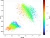 |
Fig. 1 Distributions of RRab stars considered in Paper I and RRc stars from our selected development datasets on the amplitude in the G band versus period diagram, colour-coded by metallicity. |
2.2 Phase-folding and alignment
A fundamental step in analysing periodic variable stars is phase-folding. The phase (Φ) for each observational transit was calculated using the following equation:
 (1)
(1)
where T represents the observation time (that is, the heliocentric Julian day of observation), and Epochmax and P correspond to the epoch of maximum light and the pulsation period, respectively, as provided in the Gaia DR3 vari_rrlyrae table (Clementini et al. 2023). This process aligned the light curves to a common phase reference, facilitating direct comparisons across multiple cycles of variability. Aligning the light curves to the phase of maximum light is crucial, especially for the asymmetric RRab stars, ensuring consistent feature representation for the subsequent modelling steps (see e.g. Dékány & Grebel 2022 for a detailed discussion on phase alignment).
2.3 Smoothing spline interpolation and standardisation
Gaia DR3 light curves often have uneven sampling and varying numbers of data points in the G-band, ranging from 51 to 256 in our development datasets. To create uniform input sequences suitable for DL models and to reduce observational noise, a smoothing spline interpolation was applied to each phase-folded light curve using the SciPy library’s UnivariateSpline function (Virtanen et al. 2020). In more detail, this technique is used for fitting a smooth curve to a dataset, striking a balance between accurately representing the data and minimising noise or fluctuations while standardising the number of data points across all light curves. In this context, the data consist of light curves characterised by magnitude and phase, with each light curve containing a varying number of data points. The method involves determining a function that passes near the data points while minimising the overall roughness or curvature of the curve. This approach is especially valuable when the data contain random noise, as it provides a clearer representation of underlying trends or patterns.
The smoothing spline achieves this by minimising the sum of squared deviations between the fitted curve and the data points, while imposing a penalty on the curve’s curvature. Mathematically, the problem is formulated as
 (2)
(2)
Here, f (x) is the smooth function being fitted, (xi,yi) are the data points, λ is a smoothing parameter that controls the tradeoff between adherence to the data and smoothness of the curve, and f (f″ (x))2dx penalises excessive curvature by integrating the squared second derivative of the function. The result is a continuous representation of the light curve, from which we sampled a fixed number of points (264 points for RRab and 265 points for RRc stars, uniformly distributed in phase) to standardise the length of all input sequences. This process effectively reduces noise while preserving the underlying shape of the light curve.
Following the spline interpolation and resampling, the magnitudes of each light curve were standardised. This crucial step was performed using the StandardScaler from the Scikit-learn library2 (Pedregosa et al. 2011). For each light curve, this process involves subtracting its mean magnitude (μm) and then dividing by its standard deviation of magnitudes (σm). From an astrophysical perspective, subtracting the mean magnitude effectively removes the star’s average apparent magnitude over its pulsation cycle, thus centring the light curve around zero. This allows the subsequent analysis to be independent of the star’s intrinsic luminosity, distance, and interstellar extinction, contributing to the observed mean magnitude. Subsequently, dividing by the magnitudes’ standard deviation normalises the light variation’s amplitude. This ensures that all light curves are compared on a similar scale of variability, making the model focus on the shape and morphological characteristics of the light curve (e.g. skewness, acuteness of maxima/minima) rather than the absolute amplitude of pulsation, which can vary significantly even within the same class of variable stars. This standardisation yields light curves with a mean of zero and a unit standard deviation, making them more suitable for training DL models by preventing features with larger numerical ranges from dominating the learning process. The resulting standardised light curves of RRc from our development dataset are shown in Fig. 2.
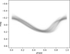 |
Fig. 2 Normalised splined G-band light curves of 6613 RRc stars from our development dataset. |
2.4 Sample weights for imbalanced data
The photometric metallicity distribution of the RRLs in our development dataset is significantly unbalanced, with a pronounced peak around —1.3 dex for RRc stars (see Fig. 3). This imbalance can bias model training, as regions of the parameter space with fewer sources contribute less to the loss function during optimisation. To address this issue, we introduced density-dependent sample weights during training.
The sample weights (wd) were computed using a Gaussian kernel density estimation approach:
 (3)
(3)
where ρ̃(x) is the normalised density estimate of the metallicity distribution at a given point (x). Gaussian kernels were used to estimate the density (ρ̃), ensuring that areas with lower data density received higher weights. These weights were normalised to ensure the sum of all weights equals the total number of samples, thereby preserving the overall loss scale.
The sample weights (wd) were integrated into the training pipeline as tensor inputs alongside the light curve data. Specifically:
The input tensor consists of the pre-processed light curve data,
 where X(t) is defined as
 (4)
(4)The sample weights tensor,
 was supplied as an additional input to the model’s loss function. In practice, this means each sample in the dataset contributes to the loss function proportionally to its assigned weight (wd).
Integrating sample weights allows the model to account for the entire range of metallicities, mitigating bias caused by overrepresented regions in the dataset. Figure 3 illustrates the photometric metallicity distribution and the corresponding sample weights for RRc stars.
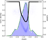 |
Fig. 3 Photometric metallicity distributions and corresponding sample weights (black lines) for RRc stars. Regions with lower data density are assigned higher weights to ensure a balanced contribution during model training. |
2.5 Improved model performance with uniform pre-processing
As demonstrated by Paper I Monti et al. (2024), pre-processing the phase-folded light curves significantly improves model performance. Applying noise reduction techniques, phase alignment, smoothing spline method, and sample weights enhances the predictive accuracy of DL models by ensuring consistent and high-quality input data. These improvements are particularly evident in regression tasks, where the pre-processing pipeline mitigates variability and biases inherent to raw observational data.
Both the RRab stars studied in Paper I and the RRc stars were subjected to the identical pre-processing pipeline, ensuring the same degree of noise reduction, phase alignment, and normalisation. Despite the intrinsic differences in their light curve shapes -sawtooth-shaped for RRab and sinusoidal for RRc, clearly recognizable only in the optical bands, where the pulsation signatures are most prominent - this unified approach guarantees comparable inputs for subsequent modelling, preserving the integrity of their physical and observational characteristics.
3 Predictive modelling
3.1 RNNs
Recurrent neural networks are a class of artificial neural networks designed to model sequential data by leveraging temporal dynamics. Unlike traditional feed-forward neural networks, RNNs incorporate recurrent connections that enable them to maintain a hidden state, capturing information from previous time steps (Williams & Zipser 1989). This capability makes RNNs well suited for tasks where the order and context of data points are critical, such as time-series analysis (Connor et al. 1994), natural language processing (Rodriguez et al. 1999), and speech recognition (Robinson et al. 1996).
Mathematically, the hidden state ht of an RNN at time t is updated as
 (5)
(5)
where xt is the input at time t, Wh and Wx are weight matrices, b is the bias, and f is a non-linear activation function, which introduces non-linearity into the network and allows it to capture complex relationships in the data, typically tanh or ReLU. The output of the RNN can either be a single value (for tasks like regression or classification) or a sequence (for tasks like translation or text generation). However, traditional RNNs face challenges such as the vanishing and exploding gradient problems, which limit their ability to learn long-term dependences in sequences. To address these issues, advanced architectures like LSTM and GRU have been developed. These architectures introduce gating mechanisms that allow the network to selectively store, forget, or update information across time steps.
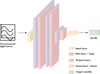 |
Fig. 4 Schematic overview of the GRU-based neural network architecture used for predicting stellar metallicity ([Fe∕H]) from pre-processed light curves. The model comprises an input layer and a sequence of GRU layers with tanh activations, interleaved with dropout layers to prevent overfitting, followed by a dense linear layer that produces the final regression output. |
3.2 GRU neural networks
The GRU, introduced by Cho et al. (2014), is a variant of the RNN designed to address the vanishing gradient problem in sequential data modelling. GRUs, like LSTM networks, capture long-term dependences but are computationally lighter due to their simplified gating mechanism. The architecture of a GRU incorporates two primary gates: the update gate and the reset gate. The update gate zt determines the amount of information from the past to retain, while the reset gate rt controls the degree of forgetting of previous states. The mathematical formulation for GRU is as follows:
![Mathematical equation: z_t &= \sigma(W_z \cdot [h_{t-1}, x_t] + b_z), \\](/articles/aa/full_html/2025/10/aa55681-25/aa55681-25-eq8.png) (6)
(6)
![Mathematical equation: r_t &= \sigma(W_r \cdot [h_{t-1}, x_t] + b_r), \\](/articles/aa/full_html/2025/10/aa55681-25/aa55681-25-eq9.png) (7)
(7)
![Mathematical equation: \tilde{h}_t &= \tanh(W_h \cdot [r_t * h_{t-1}, x_t] + b_h), \\](/articles/aa/full_html/2025/10/aa55681-25/aa55681-25-eq10.png) (8)
(8)
 (9)
(9)
where xt is the input, ht-1 is the hidden state from the previous timestep, W and b are learnable weights and biases, σ is the sigmoid activation function, and tanh is the hyperbolic tangent activation function.
Gated recurrent units are particularly effective for regression tasks involving sequential data, such as time-series prediction. To adapt GRUs for regression, the network is typically structured with a dense output layer that has a linear activation function:
 (10)
(10)
where Wo and bo are the weights and biases of the output layer, and y is the predicted continuous value.
The network is trained to minimise a loss function suitable for regression, such as the mean squared error (MSE):
 (11)
(11)
where yi and ỹi are the ground truth and predicted values, respectively. This formulation ensures that the model learns to reduce the squared deviations between predictions and observations, making it well-suited for continuous-valued targets such as metallicity estimates. The choice of GRU is further supported by our previous findings Monti et al. (2024), where nine different sequential models were evaluated, and the GRU architecture consistently yielded the best performance.
In our architecture shown in Fig. 4, each main block comprises a GRU layer followed by a dropout layer, mitigating overfitting and enhancing the model’s generalisation capabilities. This approach is pivotal in improving the performance and robustness of models handling sequential data. The final configuration of the GRU network includes three such main blocks, followed by a dense layer with linear activation:
 (12)
(12)
Here, n represents the number of main blocks, set to 3 in our design, and GRU_block refers to a block constructed using a GRU layer.
3.3 Strategies for model selection and optimisation
The development of an effective predictive model involves two fundamental stages: training and hyperparameter optimisation. During the training phase, the model’s internal parameters (weights and biases) are adjusted iteratively to minimise a chosen loss function on a dedicated training dataset. For neural networks, this minimisation is typically achieved using gradientbased optimisation algorithms (Goodfellow et al. 2016). Concurrently, hyperparameter optimisation focuses on selecting the best configuration for the model architecture and the training process itself. Hyperparameters - such as the number of layers, the number of neurons per layer, the learning rate, dropout probability, and the type of regularisation - are not learned directly from the training data but are set beforehand. Their optimal values are determined by evaluating the model’s performance on a separate validation dataset, ensuring the chosen configuration generalises well to unseen data.
For efficient hyperparameter exploration across the nine different network architectures considered, we employed the Hyperband algorithm (Li et al. 2018), as implemented in the Scikit-learn library (Pedregosa et al. 2011). The search space included dropout rates in [0.1, 0.2, 0.4, 0.6], learning rates in [0.001, 0.01, 0.1], and batch sizes in [32, 64, 128, 256, 512].
The core of the training process utilised the MSE as the loss function. Crucially, this loss was weighted using the sample weights derived in Sect. 2.4 to counteract the metallicity imbalance inherent in the RRL dataset (Fig. 3). To mitigate the risk of overfitting - where the model learns the training data too well, including its noise, and performs poorly on new data -we incorporated standard regularisation techniques. Specifically, we experimented with kernel regularisation (L1 and L2 penalties, also known as lasso and ridge penalties, applied to network weights; Tibshirani 1996; Hoerl & Kennard 1970) and dropout (Srivastava et al. 2014), which randomly sets a fraction of neuron outputs to zero during training, preventing over-reliance on specific features. The Hyperband search helped identify the optimal combination of these regularisation strategies and their associated parameters (e.g. dropout rate, L1/L2 strength) for each architecture.
Evaluating model performance during hyperparameter tuning and for final assessment requires metrics that accurately reflect prediction quality on unseen data. We used standard regression metrics: root mean squared error (RMSE) and mean absolute error (MAE) along with their weighted counterparts (wRMSE and wMAE), which incorporate the sample weights. These metrics quantify the average prediction error magnitude. Additionally, we considered the coefficient of determination (R2) score:
 (13)
(13)
where yi represents the observed value of the dependent variable for the ith observation, ỹi represents the value of the dependent variable predicted by the model for the ith observation, and ỹ represents the mean of the observed values. The R2 value ranges from 0 to 1, with 1 indicating perfect prediction and 0 indicating that it does not explain any variability in the dependent variable. Higher R2 values suggest a better model fit.
To obtain robust estimates of model performance and generalisation ability, we employed repeated stratified K-fold cross-validation. This technique extends standard K-fold crossvalidation. The dataset is divided into K folds (partitions). In each iteration, K-1 folds are used for training, and the remaining fold is used for validation. Stratification ensures that the distribution of metallicity values (the target value) is approximately preserved in each fold, which is crucial given the imbalanced nature of our data (Sect. 2.4). The entire K-fold process is repeated multiple times with different random shuffles of the data before splitting into folds. This repetition reduces the dependence of the performance estimate on the specific random splits, yielding a more reliable assessment of how the model is likely to perform on new, unseen data.
For the actual parameter updates during training, we utilised the Adam optimisation algorithm (Kingma & Ba 2014), a widely used adaptive learning rate method known for its efficiency and effectiveness in DL tasks. A fixed learning rate of 0.01 was used, selected via the hyperparameter search. Early stopping was employed as an additional regularisation measure: training was halted when performance on the validation fold ceased to improve for a predefined number of epochs, preventing overfitting by stopping before the model starts fitting noise in the training data. A mini-batch size of 256 was used to balance computational efficiency with the stochasticity needed for effective gradient descent, while ensuring that each batch provided a reasonably comprehensive representation of the metallicity range. All code developed for this study is publicly available in the open-source GitHub repository3.
Figure 5 displays the learning curves for our best-performing model (GRU; see Sect. 3.2) during the repeated stratified K-fold cross-validation process. The plots show the evolution of the error’s loss on both the training folds (red lines) and the corresponding validation fold (green lines) over the training epochs. A clear and consistent decrease in both training and validation loss is observed as training progresses, indicating that the model is effectively learning the underlying relationship between the light curve features and metallicity. Importantly, the validation loss closely tracks the training loss without significant divergence, even across different folds (indicated by the overlap and darker colours where lines coincide). This behaviour strongly suggests that the combination of our chosen model architecture (GRU), the pre-processing pipeline (Sect. 2), and the regulari-sation strategies employed (Dropout, L1 and L2 penalties, and early stopping, as discussed in Sect. 3.3) successfully prevents overfitting. The model demonstrates good generalisation capability, performing well not only on the data it was trained on but also on unseen data within the validation folds. The stability of the learning process across the multiple folds and repetitions further underscores the robustness of our training methodology and the resulting predictive model.
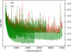 |
Fig. 5 Training (red) and validation (green) loss curves across epochs for each of the five cross-validation folds. A steady decrease in loss function indicates effective model learning, while the close alignment between training and validation loss across folds suggests good generalisation and minimal overfitting. Darker colours denote greater consistency between folds. |
Results for RRab stars, presented in Paper I, and RRc stars across various metrics for training (Train) and validation (Val) datasets using our final GRU model.
3.4 Quantitative performance evaluation
Having established the model architecture (GRU), preprocessing pipeline (Sect. 2), and optimisation strategy (Sect. 3.3), we evaluated the quantitative performance of our final predictive model for TSER of a RRL star’s metallicity. The goal was to assess how accurately the model predicts the photometric [Fe/H] values derived by Muraveva et al. (2025) based solely on the Gaia DR3 G-band light curves. The performance metrics, computed on the training and validation sets obtained through the repeated stratified K-fold cross-validation process described in Sect. 3.3, are summarised in Table 1. The results are presented separately for RRab and RRc stars.
Our optimised GRU model demonstrates high predictive accuracy and robust generalisation. The coefficient of determination R2 values are notably high: reporting from Paper I for RRab stars, R2 = 0.9447 on the training set and R2 = 0.9401 on the validation set. For RRc stars, the performance is even slightly better, with R2 = 0.9668 (training) and R2 = 0.9625 (validation). The close agreement between training and validation R2 scores, along with the high absolute values, indicates that the model effectively captures the variance in metallicity explained by the light curve features and generalises well to unseen data, avoiding significant overfitting.
The error metrics further corroborate the model’s high accuracy. As established in Paper I, the performance for RRab stars is excellent, and we report those key metrics here for completeness. In this work, we now demonstrate that our unified model achieves a similarly high level of precision for RRc stars. The wRMSE, which accounts for the metallicity distribution imbalance (Sect. 2.4), is low for both types: 0.0733 dex (RRab train), 0.0763 dex (RRab validation), 0.0679 dex (RRc train), and 0.0722 dex (RRc validation). Similarly, the wMAE values are also small, around 0.05-0.06 dex for both types and splits. The standard (unweighted) RMSE and MAE metrics show comparable low values, reinforcing the conclusion of high predictive precision across the board.
A crucial aspect of evaluating our model is comparing its performance against the current state-of-the-art. For Gaia G-band data, the relevant benchmark is the BiLSTM model presented by Dékány & Grebel (2022), which was developed exclusively for RRab stars.
As established in Paper I, our GRU model demonstrates a significant performance improvement for RRab stars. For instance, the validation wRMSE achieved by our GRU model (0.0763 dex for RRab stars) is substantially lower than the 0.13 dex reported for the BiLSTM model by Dékány & Grebel (2022), indicating a significant reduction in prediction error with our approach. Similar improvements are seen across other error metrics (wMAE, RMSE, and MAE) when comparing our RRab results in Table 1 with the results in Table 3 of Dékány & Grebel (2022).
The performance improvement over the work of Dékány & Grebel (2022) is multi-faceted, stemming from advantages in our training data, pre-processing pipeline, and model architecture. Fundamentally, our model benefits from a more recent and extensive training set derived from Gaia DR3 and the homogeneous metallicity scale of Muraveva et al. (2025). The richer DR3 data provide better-sampled light curves; as we demonstrate, there is a clear positive correlation between the number of photometric epochs and the final prediction accuracy, suggesting that the intrinsic quality of our input data allows the model to learn metallicity-sensitive features more effectively. Furthermore, our pre-processing pipeline employs techniques distinct from those in previous work. By using smoothing spline interpolation and standardising all light curves to a uniform length, we reduce observational noise and enable the model to focus on subtle morphological features relevant to metallic-ity, a different approach from the binning strategy previously employed. Finally, while our GRU architecture itself is a key component, achieving a relevant validation improvement over their BiLSTM architecture.
The primary contribution of this work, however, is the extension of this high-precision approach to RRc stars and its integration into a unified framework. As shown in Table 1, our model achieves a validation wRMSE of 0.0722 dex for RRc stars.
While a direct comparison with Dékány & Grebel (2022) is not possible for this stellar type, this result establishes a new, robust benchmark for metallicity estimation of RRc stars from light curves.
Visual confirmation of the model’s performance is provided in Fig. 6. These scatter plots compare the true (input) photometric metallicities against the values predicted by the GRU model. The figure places the results for RRab (left panel), first analysed in Paper I, alongside the new results for RRc stars (right panel), visually confirming that our single model performs with exceptional consistency across both pulsation types. In all cases, the data points cluster tightly around the identity line (y=x, shown in red), indicating excellent agreement between predicted and true values. The low amount of scatter visually confirms the low error metrics reported in Table 1 and reinforces the model’s ability to accurately regress metallicity across the studied range.
Overall, the quantitative evaluation demonstrates that our optimised GRU-based model provides highly accurate and robust predictions of photometric metallicity for both RRab and RRc stars using Gaia DR3 G -band light curves, surpassing the performance of previously published DL models for this specific task and dataset.
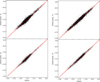 |
Fig. 6 True versus predicted photometric metallicity values from the GRU predictive model for the RRab stars presented in Paper I (left panel) and RRc stars (right panel). In each case, the top and bottom panels correspond to the training (T) and validation (V) datasets, respectively. The red lines denote the identity function. |
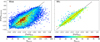 |
Fig. 7 Comparison of true photometric metallicity values from Muraveva et al. (2025) with the metallicity predicted by the GRU model for 108 766 RRab (left panel) and 13 388 RRc stars (right panel) in the test set. The dashed black lines indicate the identity function (y=x). Each point is colour-coded according to the number of G-band epochs (Nepochs) available in the Gaia DR3 catalogue for each star. |
4 Validation of photometric metallicity predictions
Having developed and optimised our GRU-based DL model for the TSER task (Sect. 3.3) and quantitatively assessed its performance using cross-validation (Sect. 3.4), we tested its performance on a final, independent test set. The goal was to understand how the model behaves across the large dataset of RRLs for which target photometric metallicities from Muraveva et al. (2025), including stars that did not meet the strict quality criteria used for training (see Sect. 2.1). In this section we present this test for both RRab and RRc stars. The results for RRab stars, which were first established and discussed in Paper I, are reported here alongside the new results for RRc stars to allow for a direct and comprehensive comparison. We also investigate factors influencing the prediction accuracy, such as pulsation type and observational sampling.
The testing process involves applying the trained GRU model to infer [Fe/H] from the Gaia DR3 G-band light curves (preprocessed as described in Sect. 2) and comparing these predictions against the target photometric metallicity values derived by Muraveva et al. (2025). It is important to recall that these target values, while serving as the ground truth for training and evaluating our specific regression model, are themselves photometric estimates calibrated using spectroscopically measured metallicities from the literature (Crestani et al. 2021; Liu et al. 2020). The comparison thus assesses how well our DL model, which utilises the full time-series information, reproduces the metallicities derived from period-Fourier parameter relations.
The left panel of Fig. 7 presents this comparison for a substantial test set comprising 108 766 RRab stars from the Gaia DR3 catalogue (Clementini et al. 2023), which were not used in model training and for which photometric metallicities are provided by Muraveva et al. (2025). The scatter plot compares the model’s predicted [Fe/H] against the true [Fe/H] values, with points colour-coded according to the number of G-band epochs (Nepochs) available in the Gaia DR3 catalogue for each star. A strong correlation around the identity line (y=x) is evident, confirming the model’s general ability to predict RRab metallicities accurately, consistent with the high R2 value reported in Table 1. However, a noticeable scatter is present, which clearly correlates with Nepochs. Stars with fewer epochs (bluish colours) exhibit significantly larger deviations from the identity line compared to those with higher epoch counts (reddish colours). This trend strongly suggests that denser temporal sampling allows the GRU model to better learn the subtle morphological features of the light curve (e.g. rise time, asymmetry, presence of bumps) that correlate with metallicity. Sparse sampling inevitably leads to poorer phase coverage and increased uncertainty in the light curve representation, hindering the model’s predictive precision. Moreover, it is important to stress that the RRab stars in the test set were not included in the training set and may have larger errors in their metallicities or φ31 parameter, or a small number of epochs (according to the selection criteria described in Sect. 2.1), and thus have less accurate photometric metallicities than the stars in the training set. These less accurate target photometric metallicities may have contributed to the scatter observed in the left panel of Fig. 7. The inherent complexity and star-tostar variability in RRab light curve shapes - for example due to the Blazhko effect (Blažko 1907), although not explicitly modelled here - may also contribute to the baseline scatter even at high epoch counts. Finally, the left panel of Fig. 7 shows an offset between the predicted and true metallicity values for RRab stars, with the predicted values being systematically lower. However, the large overall scatter makes it difficult to determine the exact cause of this offset. A more thorough analysis will be possible once additional epochs become available for each star. Gaia DR4, which will span 66 months of observations (compared to the 34 months of DR3), will almost double the number of available epochs. This will enable us to improve both the GRU model predictions and the underlying photometric metallicity estimates.
The right panel of Fig. 7 shows the analogous comparison for a large sample of 13 388 RRc stars. Visually, the correlation appears tighter, and the overall scatter around the identity line is reduced compared to the RRab sample, partly due to the significantly smaller number of stars for which this comparison was possible. The reduced scatter compared to RRab stars is consistent with the slightly better quantitative metrics obtained for RRc stars (Table 1). The improved performance for RRc stars is likely attributable to their light curve morphology. The light curves of RRc stars are more symmetric and closer to sinusoidal, and likely better sampled thanks to the shorter pulsation periods of RRc compared to RRab stars, hence presenting potentially simpler or more stable features for the model to correlate with [Fe/H]. While RRc stars can also exhibit modulation effects, their fundamental shape is less complex than that of RRab stars. This relative simplicity might make the metallicity inference less sensitive to sparse sampling or observational noise compared to the RRab stars case. Nonetheless, residual dependence on the number of epochs remains visible, although much less pronounced than for RRab stars, with higher Nepochs leading to more precise predictions.
Photometric metallicities calculated using period-Fourier parameters-metallicity relations were provided for 134769 RRLs (114 768 RRab and 20 001 RRc) by Muraveva et al. (2025). The smaller number of RRc stars is due to the limited availability of the Fourier parameter (φ31) for RRc stars in the Gaia DR3 catalogue, which is expected to significantly improve with DR4. By applying our DL model directly to the light curves, we were able to recover metallicities for 258 696 RRLs (169 024 RRab and 89 672 RRc stars) from the cleaned Gaia DR3 catalogue, increasing the number of stars with available metallicities by factors of 1.25 and 4.48 for RRab and RRc stars, respectively. This improvement has the potential to significantly enhance studies of the structure and chemical abundances of the MW and Local Group galaxies. Figure C.1 shows the sky distribution of these 258 696 RRLs, colour-coded by photometric metallic-ities derived by applying the DL model to their light curves. As expected, more metal-rich stars are concentrated in the disc of the Galaxy, while more metal-poor stars are distributed throughout the MW halo. This demonstrates the potential of the method developed in this study for future applications.
The clear dependence of prediction accuracy on the number of observational epochs, demonstrated in Fig. 7, has significant implications. Based on the trends observed in Fig. 7, we anticipate that applying our GRU model (or similar DL approaches) to Gaia DR4 light curves will yield substantially more precise photometric metallicity estimates. The reduced scatter for high-Nepochs stars in the current data suggests that improved phase coverage directly translates to better constraints on metallicity-sensitive light curve features.
More precise and accurate large-scale photometric metal-licity maps, derived from hundreds of thousands of RRLs distributed throughout the Galactic halo, bulge, and satellite systems, will enable unprecedented studies of the MW’s chemical structure, accretion history, and the properties of its oldest stellar populations (Dékány & Grebel 2022; Monti et al. 2024; Muraveva et al. 2025). Furthermore, future high-cadence, deep surveys like the Vera C. Rubin Observatory’s Legacy Survey of Space and Time (LSST) will provide light curves with even better sampling for vast numbers of faint RRLs in the southern hemisphere. These future datasets promise to further refine TSER models, pushing the boundaries of precision achievable for photometric metallicity estimation and enabling detailed chemo-dynamical studies across enormous volumes of the Galaxy.
5 Summary and conclusions
The current era of large-scale astronomical surveys, prominently featuring the Gaia mission, delivers datasets of unprecedented size and richness, necessitating the development of sophisticated computational tools for scientific analysis. RRLs stand out as essential probes of the MW’s old, metal-poor populations. Estimating their metallicity is crucial for understanding Galactic chemical evolution, yet traditional methods for measuring photometric metallicities face limitations in calibrating and capturing the nuances of light curve morphology. Addressing this, and building on the methodological framework we established for RRab stars in Paper I, we have presented and validated a unified DL framework for the TSER of photometric metallicity. Specifically, we applied a single, optimised GRU architecture to Gaia DR3 G-band light curves of both RRab and RRc stars.
Our methodology, whose technical implementation was detailed comprehensively in Paper I, integrates several critical components for robust results. A comprehensive data preparation pipeline ensures data quality through careful selection, phasefolding, and alignment appropriate for pulsating stars, smoothing spline interpolation for noise reduction and standardisation, and density-dependent sample weighting to counteract the natural metallicity imbalance of the Galactic RRL population. Rigorous hyperparameter optimisation using Hyperband, combined with effective regularisation strategies including L1 and L2 penalties, dropout, and early stopping within a repeated stratified K-fold cross-validation framework, leads to the selection of an optimised GRU model.
This final GRU model has high predictive accuracy and strong generalisation capabilities. As first reported in Paper I, the model achieves excellent performance for RRab stars (R2 ≈ 0.94, wRMSE ≈ 0.076 dex). In this work we have shown that our unified model extends these results to RRc stars, achieving an even higher precision (R2 ≈ 0.96, wRMSE ≈ 0.072 dex).
Taken together, these results represent a significant improvement in precision compared to previous DL benchmarks applied to Gaia G-band data (Dékány & Grebel 2022). Furthermore, our test analysis explicitly quantified the positive impact of increased observational sampling; light curves with a higher number of epochs in the G band consistently yield more precise metallicity predictions. Finally, the application of our DL model directly to the light curves allowed us to increase the number of stars with available metallicities by factors of 1.25 and 4.48 for RRab and RRc stars, respectively.
The success of this unified GRU-based TSER approach highlights the broader potential of DL applied to modern astronomical time series. Deriving accurate photometric metallicities directly from light curves offers a scalable and computationally efficient pathway for chemically characterising vast numbers of RRLs, complementing or replacing more resource-intensive spectroscopic methods. This enables the construction of large, homogeneous metallicity catalogues directly linked to Gaia’s photometry and astrometry, facilitating detailed investigations into the structure, formation history, and chemical enrichment patterns of the MW and Local Group galaxies.
Looking forward, the demonstrated dependence on data sampling suggests that substantial gains in precision can be achieved with upcoming datasets. Gaia DR4, with its longer time baseline and a nearly twice the amount of epoch data compared to DR3 (Gaia Collaboration 2023), and the future deep, high-cadence observations from the Vera C. Rubin Observatory’s LSST, will provide significantly richer light curves. Our future work will aim to leverage these resources by expanding the scope of our models to potentially include more different photometric bands, further refining the DL architectures, perhaps through attention mechanisms or transformers, and ultimately applying the derived high-precision metallicity catalogues to pressing questions in Galactic archaeology and chemo-dynamics.
Data availability
Full Table A.1 is available at the CDS via https://cdsarc.cds.unistra.fr/viz-bin/cat/J/A+A/702/A148.
Acknowledgements
This work uses data from the European Space Agency mission Gaia (https://www.cosmos.esa.int/gaia), processed by the Gaia Data Processing and Analysis Consortium (DPAC; https://www.cosmos.esa.int/web/gaia/dpac/consortium). Funding for the DPAC has been provided by national institutions, in particular the institutions participating in the Gaia Multilateral Agreement. Support to this study has been provided by INAF Mini-Grant (PI: Tatiana Muraveva), by the Agenzia Spaziale Italiana (ASI) through contract ASI 2018-24-HH.0 and its Addendum 2018-24-HH.1-2022, and by Premiale 2015, Mining The Cosmos - Big Data and Innovative Italian Technology for Frontiers Astrophysics and Cosmology (MITiC; PI: B.Garilli). This research was also supported by the International Space Science Institute (ISSI) in Bern, through ISSI International Team project #490, ‘SHOT: The Stellar Path to the H0 Tension in the Gaia, Transiting Exoplanet Survey Satellite (TESS), Large Synoptic Survey Telescope (LSST), and James Webb Space Telescope (JWST) Era’ (PI: G. Clementini).
References
- Belokurov, V., Evans, N. W., & Du, Y. L. 2003, MNRAS, 341, 1373 [Google Scholar]
- Belokurov, V., Evans, N. W., & Le Du, Y. 2004, MNRAS, 352, 233 [Google Scholar]
- Belokurov, V., Deason, A., Koposov, S., et al. 2018, MNRAS, 477, 1472 [Google Scholar]
- Blazko, S. 1907, Astron. Nachr., 175, 325 [NASA ADS] [CrossRef] [Google Scholar]
- Bobrick, A., Iorio, G., Belokurov, V., et al. 2024, MNRAS, 527, 12196 [Google Scholar]
- Chadid, M., Sneden, C., & Preston, G. W. 2017, ApJ, 835, 187 [Google Scholar]
- Cho, K., Van Merriënboer, B., Gulcehre, C., et al. 2014, arXiv e-prints [arXiv:1406.1078] [Google Scholar]
- Clementini, G., Carretta, E., Gratton, R., et al. 1995, AJ, 110, 2319 [Google Scholar]
- Clementini, G., Cignoni, M., Contreras Ramos, R., et al. 2012, ApJ, 756, 108 [NASA ADS] [CrossRef] [Google Scholar]
- Clementini, G., Ripepi, V., Molinaro, R., et al. 2019, A&A, 622, A60 [NASA ADS] [CrossRef] [EDP Sciences] [Google Scholar]
- Clementini, G., Ripepi, V., Garofalo, A., et al. 2023, A&A, 674, A18 [NASA ADS] [CrossRef] [EDP Sciences] [Google Scholar]
- Connor, J. T., Martin, R. D., & Atlas, L. E. 1994, IEEE Trans. Neural Netw., 5, 240 [Google Scholar]
- Crestani, J., Fabrizio, M., Braga, V. F., et al. 2021, ApJ, 908, 20 [Google Scholar]
- Dall’Ora, M., Clementini, G., Kinemuchi, K., et al. 2006, ApJ, 653, L109 [CrossRef] [Google Scholar]
- Debosscher, J., Sarro, L., Aerts, C., et al. 2007, A&A, 475, 1159 [NASA ADS] [CrossRef] [EDP Sciences] [Google Scholar]
- Dékány, I., & Grebel, E. K. 2022, ApJS, 261, 33 [CrossRef] [Google Scholar]
- Dékány, I., Grebel, E. K., & Pojmanski, G. 2021, ApJ, 920, 33 [CrossRef] [Google Scholar]
- D’Orazi, V., Storm, N., Casey, A. R., et al. 2024, MNRAS, 531, 137 [CrossRef] [Google Scholar]
- Drake, A., Catelan, M., Djorgovski, S., et al. 2013, ApJ, 763, 32 [NASA ADS] [CrossRef] [Google Scholar]
- Fabrizio, M., Braga, V. F., Crestani, J., et al. 2021, ApJ, 919, 118 [NASA ADS] [CrossRef] [Google Scholar]
- Gaia Collaboration (Prusti, T., et al.) 2016, A&A, 595, A1 [NASA ADS] [CrossRef] [EDP Sciences] [Google Scholar]
- Gaia Collaboration (Vallenari, A., et al.) 2023, A&A, 674, A1 [NASA ADS] [CrossRef] [EDP Sciences] [Google Scholar]
- Garofalo, A., Cusano, F., Clementini, G., et al. 2013, ApJ, 767, 62 [NASA ADS] [CrossRef] [Google Scholar]
- Garofalo, A., Tantalo, M., Cusano, F., et al. 2021, ApJ, 916, 10 [NASA ADS] [CrossRef] [Google Scholar]
- Gilligan, C. K., Chaboyer, B., Marengo, M., et al. 2021, MNRAS, 503, 4719 [Google Scholar]
- Goodfellow, I., Bengio, Y., Courville, A., & Bengio, Y. 2016, Deep learning (Cambridge: MIT Press) [Google Scholar]
- Hajdu, G., Dékány, I., Catelan, M., Grebel, E. K., & Jurcsik, J. 2018, ApJ, 857, 55 [Google Scholar]
- Hoerl, A. E., & Kennard, R. W. 1970, Technometrics, 12, 55 [Google Scholar]
- Iorio, G., & Belokurov, V. 2019, MNRAS, 482, 3868 [NASA ADS] [CrossRef] [Google Scholar]
- Iorio, G., & Belokurov, V. 2021, MNRAS, 502, 5686 [Google Scholar]
- Jurcsik, J., & Kovacs, G. 1996, A&A, 312, 111 [Google Scholar]
- Kingma, D. P., & Ba, J. 2014, arXiv e-prints [arXiv:1412.6980] [Google Scholar]
- Li, L., Jamieson, K., DeSalvo, G., Rostamizadeh, A., & Talwalkar, A. 2018, J. Mach. Learn. Res., 18, 1 [Google Scholar]
- Li, X.-Y., Huang, Y., Liu, G.-C., Beers, T. C., & Zhang, H.-W. 2023, ApJ, 944, 88 [NASA ADS] [CrossRef] [Google Scholar]
- Liu, G. C., Huang, Y., Zhang, H. W., et al. 2020, ApJS, 247, 68 [NASA ADS] [CrossRef] [Google Scholar]
- Mahabal, A., Djorgovski, S., Turmon, M., et al. 2008, Astron. Nachr: Astron. Notes, 329, 288 [Google Scholar]
- Molnár, L., Pál, A., Plachy, E., et al. 2015, ApJ, 812, 2 [Google Scholar]
- Monti, L., Muraveva, T., Clementini, G., & Garofalo, A. 2024, Sensors, 24, 5203 [Google Scholar]
- Morgan, S. M., Wahl, J. N., & Wieckhorst, R. M. 2007, MNRAS, 374, 1421 [NASA ADS] [CrossRef] [Google Scholar]
- Muraveva, T., Clementini, G., Garofalo, A., & Cusano, F. 2020, MNRAS, 499, 4040 [NASA ADS] [CrossRef] [Google Scholar]
- Muraveva, T., Giannetti, A., Clementini, G., Garofalo, A., & Monti, L. 2025, MNRAS, 536, 2749 [Google Scholar]
- Nemec, J. M., Cohen, J. G., Ripepi, V., et al. 2013, ApJ, 773, 181 [CrossRef] [Google Scholar]
- Pancino, E., Britavskiy, N., Romano, D., et al. 2015, MNRAS, 447, 2404 [Google Scholar]
- Pedregosa, F., Varoquaux, G., Gramfort, A., et al. 2011, J. Mach. Learn. Res., 12, 2825 [Google Scholar]
- Preston, G. W. 1959, ApJ, 130, 507 [Google Scholar]
- Richards, J. W., Starr, D. L., Butler, N. R., et al. 2011, ApJ, 733, 10 [NASA ADS] [CrossRef] [Google Scholar]
- Robinson, T., Hochberg, M., & Renals, S. 1996, in Automatic Speech and Speaker Recognition: Advanced Topics (Springer), 233 [Google Scholar]
- Rodriguez, P., Wiles, J., & Elman, J. L. 1999, Connect. Sci., 11, 5 [Google Scholar]
- Sesar, B., Banholzer, S. R., Cohen, J. G., et al. 2014, ApJ, 793, 135 [NASA ADS] [CrossRef] [Google Scholar]
- Skowron, D. M., Soszynski, I., Udalski, A., et al. 2016, Acta Astron., 66, 269 [Google Scholar]
- Smith, H. A. 2004, RR Lyrae Stars (Cambridge University Press) [Google Scholar]
- Smolec, R. 2005, Acta Astron., 55, 59 [NASA ADS] [Google Scholar]
- Srivastava, N., Hinton, G., Krizhevsky, A., Sutskever, I., & Salakhutdinov, R. 2014, J. Mach. Learn. Res., 15, 1929 [Google Scholar]
- Tan, C. W., Bergmeir, C., Petitjean, F., & Webb, G. I. 2021, Data Mining Knowl. Discov., 35, 1032 [Google Scholar]
- Tibshirani, R. 1996, J. Roy. Statist. Soc. Ser. B: Statist. Methodol., 58, 267 [CrossRef] [Google Scholar]
- Virtanen, P., Gommers, R., Oliphant, T. E., et al. 2020, Nat. Methods, 17, 261 [Google Scholar]
- Willemsen, P., & Eyer, L. 2007, arXiv e-prints [arXiv:0712.2898] [Google Scholar]
- Williams, R. J., & Zipser, D. 1989, Neural Computat., 1, 270 [Google Scholar]
- WoZniak, P., Williams, S., Vestrand, W., & Gupta, V. 2004, ApJ, 128, 2965 [Google Scholar]
Appendix A Datasets
Parameters of 6002 RRab (a) and 6613 RRc (b) stars from the Gaia DR3 catalogue (Clementini et al. 2023) selected as discussed in Sect. 2.1 (extract).
Appendix B Computational environment
The training and evaluation of the DL models described in this work were computationally intensive, requiring specialised hardware. All experiments were conducted on a high-performance workstation equipped with an NVIDIA GeForce RTX 4070 graphics processing unit (GPU), featuring 12GB of video RAM (VRAM), specifically chosen for its capability to accelerate the matrix operations inherent in neural network training. The system was further configured with 32GB of DDR5 RAM for efficient data handling and a high-speed non-volatile memory express (NVMe) solid-state drive to minimise data loading bottlenecks during training.
The software environment comprised Python 3.10 with TensorFlow 2.13.0, accessed via the Keras API version 2.13.1, for model definition, training, and evaluation. To leverage the GPU’s computational power, the CUDA Toolkit version 11.8 and the NVIDIA CUDA Deep Neural Network library version 8.6 were used. This specific software stack ensured optimised performance and compatibility between the hardware and the DL libraries, facilitating efficient execution of the training and hyperparameter optimisation procedures outlined in Sect. 3.3.
Appendix C All-sky map of Gaia DR3 RR Lyrae stars by photometric metallicity
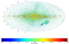 |
Fig. C.1 Sky distribution of 258 696 RRLs from the cleaned Gaia DR3 sample, colour-coded by photometric metallicities derived using the GRUbased predictive model. |
All Tables
Results for RRab stars, presented in Paper I, and RRc stars across various metrics for training (Train) and validation (Val) datasets using our final GRU model.
Parameters of 6002 RRab (a) and 6613 RRc (b) stars from the Gaia DR3 catalogue (Clementini et al. 2023) selected as discussed in Sect. 2.1 (extract).
All Figures
|
Fig. 1 Distributions of RRab stars considered in Paper I and RRc stars from our selected development datasets on the amplitude in the G band versus period diagram, colour-coded by metallicity. |
| In the text | |
|
Fig. 2 Normalised splined G-band light curves of 6613 RRc stars from our development dataset. |
| In the text | |
|
Fig. 3 Photometric metallicity distributions and corresponding sample weights (black lines) for RRc stars. Regions with lower data density are assigned higher weights to ensure a balanced contribution during model training. |
| In the text | |
|
Fig. 4 Schematic overview of the GRU-based neural network architecture used for predicting stellar metallicity ([Fe∕H]) from pre-processed light curves. The model comprises an input layer and a sequence of GRU layers with tanh activations, interleaved with dropout layers to prevent overfitting, followed by a dense linear layer that produces the final regression output. |
| In the text | |
|
Fig. 5 Training (red) and validation (green) loss curves across epochs for each of the five cross-validation folds. A steady decrease in loss function indicates effective model learning, while the close alignment between training and validation loss across folds suggests good generalisation and minimal overfitting. Darker colours denote greater consistency between folds. |
| In the text | |
|
Fig. 6 True versus predicted photometric metallicity values from the GRU predictive model for the RRab stars presented in Paper I (left panel) and RRc stars (right panel). In each case, the top and bottom panels correspond to the training (T) and validation (V) datasets, respectively. The red lines denote the identity function. |
| In the text | |
|
Fig. 7 Comparison of true photometric metallicity values from Muraveva et al. (2025) with the metallicity predicted by the GRU model for 108 766 RRab (left panel) and 13 388 RRc stars (right panel) in the test set. The dashed black lines indicate the identity function (y=x). Each point is colour-coded according to the number of G-band epochs (Nepochs) available in the Gaia DR3 catalogue for each star. |
| In the text | |
|
Fig. C.1 Sky distribution of 258 696 RRLs from the cleaned Gaia DR3 sample, colour-coded by photometric metallicities derived using the GRUbased predictive model. |
| In the text | |
Current usage metrics show cumulative count of Article Views (full-text article views including HTML views, PDF and ePub downloads, according to the available data) and Abstracts Views on Vision4Press platform.
Data correspond to usage on the plateform after 2015. The current usage metrics is available 48-96 hours after online publication and is updated daily on week days.
Initial download of the metrics may take a while.