| Issue |
A&A
Volume 702, October 2025
|
|
|---|---|---|
| Article Number | A150 | |
| Number of page(s) | 9 | |
| Section | The Sun and the Heliosphere | |
| DOI | https://doi.org/10.1051/0004-6361/202555908 | |
| Published online | 20 October 2025 | |
Magnetic interaction analysis of multiple interplanetary coronal mass ejections that led to a historic geomagnetic storm in May 2024
1
NASA Postdoctoral Program Fellow, NASA Goddard Space Flight Center, Greenbelt, MD 20771, USA
2
Heliophysics Science Division, NASA Goddard Space Flight Center, Greenbelt, MD 20771, USA
3
The Catholic University of America, Washington, DC 20064, USA
4
Department of Physics, University of Helsinki, P.O. Box 64 FI-00014 Helsinki, Finland
5
Centre for Space Science and Technology, Indian Institute of Technology Roorkee, Roorkee, 247667 Uttarakhand, India
⋆ Corresponding author: This email address is being protected from spambots. You need JavaScript enabled to view it.
Received:
12
June
2025
Accepted:
22
August
2025
Abstract
Context. Interplanetary coronal mass ejections (ICMEs) are large-scale eruptive phenomena capable of shedding a huge amount of solar magnetic helicity and energy and can potentially drive strong geomagnetic storms. They complexly evolve while preceded and followed by other large-scale structures, such as ICMEs. Magnetic interaction among multiple ICMEs may result in intense and long-lived geomagnetic storms.
Aims. Our aim is to understand the reason for the substantial changes in the geoeffectivity of two meso-scale separated counterparts of a complex solar wind structure by investigating their magnetic content, helicity, and energy as well as their magnetic interaction among multiple ICMEs.
Methods. We utilized the in situ observations of solar wind from the Wind and the Solar Terrestrial Relations Observatory-A (STA) spacecraft during the strongest geomagnetic storm period in past two decades on May 10-11, 2024. We performed heliospheric imaging analysis to locate the solar sources, investigated the interplanetary propagation and Earth-arrival of the driver, and performed a time-frequency domain analysis of the in situ magnetic field vectors in injection and inertial ranges of magnetohydrodynamic (MHD) turbulence to quantify the driver’s magnetic content at two counterparts.
Results. Our investigation confirms complex interactions among five ICMEs resulting in distinct counterparts within a coalescing large-scale structure. These counterparts possess substantially different magnetic content.
Conclusions. We conclude that the STA-observed complex counterpart resulted from the interaction among common-origin ICMEs favorably orientated for magnetic reconnection, had a 1.6 and 2.8 times higher total magnetic energy and helicity, respectively, than the Wind-observed counterpart that included a left-handed filament-origin ICME. The left-handed ICME non-favorably oriented for magnetic reconnection with the surrounding right-handed common-origin ICMEs at Wind. Therefore, despite belonging to a common solar wind structure, two medium-separated counterparts had the potential to lead to different geoeffectivity. This ultimately challenges space weather predictions based on early observations.
Key words: Sun: coronal mass ejections (CMEs) / Sun: heliosphere / Sun: magnetic fields / solar-terrestrial relations / solar wind
© The Authors 2025
 Open Access article, published by EDP Sciences, under the terms of the Creative Commons Attribution License (https://creativecommons.org/licenses/by/4.0), which permits unrestricted use, distribution, and reproduction in any medium, provided the original work is properly cited.
This article is published in open access under the Subscribe to Open model. This email address is being protected from spambots. You need JavaScript enabled to view it. to support open access publication.
1. Introduction
Interplanetary coronal mass ejections (ICMEs, e.g., Kilpua et al. 2017) are the heliospheric manifestation of large-scale eruptive solar phenomena that impulsively release excess magnetic energy stored in twisted solar coronal field lines (e.g., Pal et al. 2017). As they depart from the corona and propagate through the heliosphere, they experience complex interactions with the surrounding plasma and magnetic fields that may lead to the significant evolution and distortion of their structure (e.g., Weiss et al. 2024; Pal et al. 2023; Braga et al. 2022), deceleration and/or acceleration (e.g., Shen et al. 2012), reconfiguration, magnetic flux erosion (e.g., Pal et al. 2022a, 2021, 2020), and accumulation of magnetic field lines (e.g., Takahashi & Shibata 2017; Kilpua et al. 2017). The physical processes driving the solar magnetic field, their emergence and variability, their manifestation as eruptive events that causally connect the Sun–geospace environment, and processes leading to the complex evolution of large-scale eruptions in the heliosphere have been reviewed by Nandy et al. (2023), Manchester et al. (2017) and Luhmann et al. (2020).
Studying interacting ICMEs has attracted interest, as ICMEs provide an ideal opportunity to investigate the complexity of space plasma, such as the propagation of a shock wave within a magnetically dominated structure (Lugaz et al. 2005, 2009; Pal et al. 2023), and magnetic and non-magnetic interactions among large-scale structures (Schmidt & Cargill 2004; Telloni et al. 2021, 2020b). Furthermore, interacting ICMEs may result in intense and long-lived geomagnetic storms (Farrugia et al. 2006a,b; Xie et al. 2006; Liu et al. 2014) by embedding extended periods of a strong southward-directed magnetic field vector Bz (Wang et al. 2003). With numerical simulations, Schmidt & Cargill (2004) have explained the different nature of the interactions among ICMEs, for example, magnetic interaction and non-elastic collision. An equalization of speeds is achieved in all interacting ICMEs regardless of the type of interactions. A magnetic interaction between ICMEs depends on their relative trajectories and sense of magnetic field topology. When two ICMEs have parallel axes with the same sense of magnetic field rotation, magnetic reconnection occurs at their interface, resulting in a single complex magnetic structure (Lugaz et al. 2013). However, if field line characteristics do not allow for reconnection, the ICMEs collide in a highly non-elastic manner. They distort around each other due to the compressibility nature of their magnetized plasma.
In general, ICMEs embed highly twisted magnetic field lines (Nieves-Chinchilla et al. 2023) and can be unambiguously identified in the in situ data as regions of high magnetic helicity (Hm) and energy (Em). The Hm is a measure of the field line twist or writhe (Moffatt 1978), and it cannot be achieved without information of the topological (spatial) properties of field lines. Telloni et al. (2012) advanced a novel technique provided by Matthaeus & Goldstein (1982) to compute the reduced Hm from the Fourier transform of the magnetic field auto-correlation matrix. While the trace of the symmetric part of the spectral matrix measures the Em, the imaginary part of the matrix measures the Hm (Batchelor 1953; Montgomery & Turner 1981; Matthaeus & Goldstein 1982). This advanced technique has been widely used in recent studies (e.g., Telloni et al. 2013, 2016, 2019; Zhao et al. 2020, 2021; Telloni et al. 2020b, 2023; Alberti et al. 2022) to identify and investigate the magnetohydrodynamics (MHD) properties of helical field lines in the solar wind.
The complexity of the magnetic field structure within ICME ejecta varies significantly from case to case, and therefore, their identification may be challenging (Al-Haddad & Lugaz 2025). At Earth, they reach a radial extension of about 0.25 au (Klein & Burlaga 1982) with a timescale ranging up to 64 hours (Telloni et al. 2019). Although a southward magnetic vector within ICMEs is essential to driving a geomagnetic storm, this is not a sufficient condition, as it is also necessary that the ICME carries a considerable amount of energy (kinetic or magnetic) to ensure an efficient energy release during the storm. An automated scheme to detect ICMEs in solar wind and assess their geoeffectiveness using helicity and energy spectrum analysis has been implemented successfully (Telloni et al. 2019). A greater amount of available ICME magnetic energy during its reconnection with the geomagnetic field allows more efficient energy release into the magnetosphere. This energy may transform to kinetic and thermal energy that further results in the acceleration of particles and increased density in the Earth’s upper atmosphere. This may result in serious disruptions in satellite signal propagation, radio communication, and positioning systems and additional drag to satellites, thus possibly changing their orbits (Baruah et al. 2024; Oliveira et al. 2025). Therefore, immense efforts have been employed to reliably detect and predict ICME-driven space weather using data-driven MHD simulations (e.g., Zhang et al. 2023), hybrid empirical and physics based MHD models (e.g., Owens et al. 2008; Mayank et al. 2024), data-constrained analytical methods (e.g., Kay et al. 2022; Sarkar et al. 2020; Pal et al. 2022b; Palmerio et al. 2021), and physics-based artificial intelligence techniques (e.g., Pal et al. 2024; Rüdisser et al. 2025; Narock et al. 2024).
The recent May 2024 storm was one of the largest geomagnetic storms that has happened since the beginning of the space age in 1957, with the disturbance storm time (Dst) index reaching at a minimum of −412 nT at 02:00 UTC on May 11 (Díaz 2025). In total, only 11 great geomagnetic storms with Dst ≤ 350 nT (Gonzalez et al. 2011) have occurred since the start of the space era. The associated structured solar wind was probed simultaneously by spacecraft at Lagrangian (L)-1 and the Solar Terrestrial Relations Observatory-A (STA), which was 12.6° westward and 1.5° northward from the Sun-Earth line. The impacts of this storm on Earth’s upper atmosphere and geomagnetically induced current (GIC) have been extensively studied (e.g., Zakharenkova et al. 2025; Clilverd et al. 2025; Zhang et al. 2025b; Ang et al. 2025; Wan et al. 2025; Zhang et al. 2025a; Tulasi Ram et al. 2024). Recent studies (e.g., Liu et al. 2024; Wang et al. 2024; Hayakawa et al. 2025; Thampi et al. 2025; Weiler et al. 2025; Kwak et al. 2024; Khuntia et al. 2025) have provided detailed analyses of event-related solar origins, connections between solar and interplanetary counterparts, thermodynamics and evolution of CME-CME interactions, and simulated ICME propagation and their arrival. Using two empirical formulas provided by O’Brien & McPherron (2000) and Burton et al. (1975), Liu et al. (2024) estimate that the ICME structure observed at STA would have caused the minimum Dst (Dstmin) that was almost ∼116 nT lower than observed at Earth. Furthermore, their estimated Dstmin was 8% smaller than the observed Dstmin at Earth.
A complex structured solar wind may appear with substantial differences in multipoint observations with meso-scale separations (Pal et al. 2023; Lugaz et al. 2025; Palmerio et al. 2024), which lead to difficulties in making reliable predictions of their occurrence. In this work, we utilize the occasion of multipoint meso-scale separated probing of a very complex solar wind structure and derive differences in their magnetic content potential to drive geoeffectivity at two probing locations. We address the reason for the highlighted differences using multiple ICME-ICME interaction phenomena. Furthermore, we attempt to explain why two moderately separated counterparts belonging to a highly structured solar wind exhibit significantly different geoeffectiveness. In Section 2, we provide details of the data and method of our analysis. Section 3 presents the results and an analysis of them. Finally, in Section 4, we discuss and conclude our study.
2. Data and methodology
For this study, we used multipoint in situ observations from the Magnetic Field Investigation (Lepping et al. 1995), Solar Wind Experiment (SWE; Ogilvie et al. 1995), and 3D Plasma Analyzer (3DP; Lin et al. 1995) instruments on board Wind. We used the Magnetometer (MAG), Solar Wind Electron Analyser (SWEA) of In situ Measurements of Particles, the CME Transients (IMPACT) suite (Acuña et al. 2008), and Plasma and Suprathermal Ion Composition (PLASTIC) instrument (Galvin et al. 2008) on board STA. We used remote sensing observations from heliospheric imagers (HI1 and HI2) and COR2 of the Sun-Earth Connection Coronal and Heliospheric Investigation (SECCHI: Howard et al. 2008) suite on board STA. We obtained science-level in situ data from NASA’s Coordinated Data Analysis Web (CDAWeb) with the highest available resolution. As the Level 2 IMPACT/MAG data had a significant data gap, we decided to use Level 1 MAG data with the highest resolution (eight samples/sec) in this work.
We followed the method for obtaining solar wind magnetic helicity (Telloni et al. 2012),
![Mathematical equation: $$ \begin{aligned} H_m(k,t) = 2\mathfrak{I} [W_y^*(k,t). W_z(k,t)]/k, \end{aligned} $$](/articles/aa/full_html/2025/10/aa55908-25/aa55908-25-eq1.gif) (1)
(1)
and normalized helicity (Telloni et al. 2013),
![Mathematical equation: $$ \begin{aligned} \sigma _m(k,t)=\frac{2\mathfrak{I} [W_y^*(k,t). W_z(k,t)]}{|W_x{k,t}|^2+|W_y{k,t}|^2+|W_z{k,t}|^2}, \end{aligned} $$](/articles/aa/full_html/2025/10/aa55908-25/aa55908-25-eq2.gif) (2)
(2)
where Wx, Wy, and Wz represent the Morlet wavelet transform of xgse, ygse, and zgse magnetic field components in the geocentric solar ecliptic (GSE) coordinate system and k is the wave number. This tool extends a spectrum-based formula of helicity derivation by Matthaeus & Goldstein (1982) to the time domain and thus allows for proper localization of magnetic helicity structures in solar wind. The tool has been used extensively to study the MHD properties of ICMEs (Telloni et al. 2013, 2016, 2019, 2020b, 2021). While Hm(k, t)∼0 indicates untwisted field lines, Hm(k, t) > 0 ( < 0) corresponds to counter-clockwise (clockwise) field line rotation in the outward magnetic sector and Hm(k, t) < 0 ( > 0) corresponds to counter-clockwise (clockwise) field line rotation in the inward magnetic sector. An ejecta of intrinsic right-handed (left-handed) helicity has been observed to have a positive (negative) value of Hm(k, t), which indicates a counter-clockwise (clockwise) rotation of field lines in an outward magnetic sector in the heliosphere.
Utilizing the Morlet wavelet transform (W) of B, we derived the magnetic energy spectrum, Em(k, t), of the solar wind following Telloni et al. (2019):
 (3)
(3)
Thus, the total magnetic energy in the solar wind can be calculated with EM(t) = ∫k5/3Em(k, t)dk. Here, by multiplying k5/3 to Em(k, t), we compensated Em(k, t) to highlight small-scale high-energy structures in solar wind because magnetic field fluctuations exhibit a 5/3 Kolmogorov-like spectrum (Telloni et al. 2019). Similarly, while estimating the total helicity Hm(t) = ∫k8/3|Hm(k, t)|, we multiplied 8/3 to Hm(k, t) to highlight the small-scale helicity structures in the helicity spectrum as it drops off with k−8/3 (Matthaeus & Goldstein 1982; Bruno & Dobrowolny 1986). Values of |Hm| and Em greater than the two standard deviations of the mean unperturbed solar wind condition are considered as the threshold to identify ICMEs in solar wind (Telloni et al. 2019).
To correlate in situ detections with their associated CMEs, we predicted the arrival time of these structures using STEREO/SECCHI data and the harmonic mean (HM) method. This method assumes a circular geometry for the CME front, anchored to the Sun, and can be used to compute the velocity, propagation angle, and arrival time of an ICME, (see, e.g., Lugaz 2010; Möstl et al. 2011). We implement this fitting using the Solar Angle-Time plot SATPLOT software tool, which generates a plot of elongation angle versus time (J-maps) from SECCHI COR2 and HI1 and HI2 data to track solar wind heliospheric structures and subsequently apply a fitting method to them to predict their arrival and impact on spacecraft in the heliosphere. The SATPLOT is available in the SECCHI software tree of SolarSoft (Freeland & Handy 1998).
3. Results and analysis
3.1. Event overview
Several studies have attempted to connect ICME ejecta observed in situ during May 10-11, 2024, to their solar origins. A total of six CMEs have been identified with suitable speeds and source positions to potentially encounter the Earth and/or STEREO-A. The details of these CMEs, taken from the studies by Liu et al. (2024)(L) and Khuntia et al. (2025)(K) implementing the graduated cylindrical shell technique (GCS, Thernisien et al. 2006; Thernisien 2011) to the coronagraph observations onboard Solar and Heliospheric Observatory (SOHO) and STA spacecraft, are provided in Table 1. An association has been found with two M-class and three X-class flares originating from AR13664, which was a super active region exhibiting extreme activity, producing 23 X-class and multiple M-class flares (Jaswal et al. 2025) and a quiet-Sun left-handed filament (Weiler et al. 2025; Martin 1998) located to the south of the AR13667. In the “Associated CMEs” column of Table 1, except for the propagation direction, we noticed a significant disagreement in CME physical parameters between different studies. This could be related to the separation between the SOHO and STA spacecraft being too far from the ideal to reliably perform the multi-spacecraft GCS fitting (Bosman et al. 2012).
Helicity localized regions in the in situ solar wind during May 10-11, 2024.
In Figure 1, we provide in situ observations of solar wind magnetic and plasma properties, including the magnetic field longitude angle (ϕ), magnetic field intensity (B), and vectors Bx, By, and Bz in GSE coordinates, bulk speed (Vsw), proton number density (Np), alpha to proton number density ratio (Na/Np), proton temperature (Tp), with the expected ambient temperature Tex (shown using a yellow line over-plotted on the Tp panel), derived from the correlation between Vsw and Tp (Lopez 1987), the ratio of plasma thermal pressure to the magnetic pressure (β), suprathermal electron pitch angle distribution (PAD), Hm and Em spectra, and the total magnetic energy derived from Wind and STA covering the peak activity solar wind period during May 10, 12:00 UT–May 11, 23:00 UT. While Wind had an uninterrupted plasma and magnetic data coverage during the investigated solar wind period, STA had many plasma data gaps. To perform a magnetic analysis of solar wind during the peak activity period, we analyzed Hm(k, t) and Em(k, t) in the injection frequency range that corresponds to the larger-scale sized structures in solar wind. We investigated the localization of helicity in solar wind during May 10-11, 2024, in both Wind and STA observations in a timescale of 0.5–64 hours corresponding to frequency domain ∼4.6e−6 − ∼5.5e−4 Hz. We provide the Hm and Em spectra in Figure 1a and b obtained from Wind and STA, respectively, where the white contours enclose the highly helical regions having |Hm|≥1/e|Hm|max. In the Em spectrum, the white contour encloses regions corresponding to  , where
  is the mean of Em of unperturbed solar wind. The contours in Hm and scale size corresponding to the highest Hm value helped us assess the time extent and scale sizes, ΔS, of ejecta cores with the maximum winding of field lines, respectively.
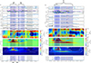 |
Fig. 1. In situ observation during May 10-11, 2024, using (a) MAG and SWE instruments on board Wind and (b) MAG, SWEA, and PLASTIC instruments on board the STA spacecraft. The dotted lines in the ϕ panel indicate the nominal sector boundaries of the interplanetary magnetic field derived using a Parker spiral angle obtained from the local solar wind observations at Wind and STA. Here, ϕ values between (outside) the lines indicate the magnetic field in the away (toward) sector of the heliosphere. The blue shaded regions of W1, W2, and S1 present the localized helicity regions in both the time and frequency domains (see Section 3.2 for details). The hatched intervals indicate an unperturbed core of ejecta, as discussed in Section 3.3. The eighth (seventh) column in panel a (b) shows the energy flux (phase space density) of suprathermal electrons in the 265 (247) eV energy bin. |
3.2. Complex solar wind intervals detected by Wind and STA
During the majority of the shown intervals, the magnetic helicity is close to zero. The Wind spacecraft, however, observed localized patches of positive and negative helicity, with |Hm| being two standard deviations higher than the average |Hm| of the unperturbed solar wind. The helicity patches were in a mostly outward magnetic field sector, revealing counter-clockwise and clockwise rotations with the size ΔS of the characteristic scale corresponding to the strong winding of magnetic field lines around its axis equal 3.2 h and 2.4 h and average σm = 0.8 ± 0.07 and −0.71 ± 0.11, respectively. The blue shaded intervals in Figure 1 labeled as W1 and W2 represent the temporal extensions of the helicity patches. The W1 region contains comparatively strongly wrapping B with maximum mean helicity, multiple intervals with lower Np, Tp < Tex, β < 0.1, and Na/Np peaks representing the presence of multiple ejecta and corresponding to the highest EM(t) value during May 10-15, 2024. Region W2 features comparatively loosely wrapping left-handed rotating field lines with three intervals of Tp < Tex and β < 0.1 and a couple of intervals with a lower Np unambiguously identified. The corresponding helicity and energy of the region are less than that of W1.
At 12.6° west and 1.5° north from the Wind location (L1), STA observed different features in Hm spectrum than those observed by Wind. Here, a tightly wound magnetic field forms a complex ejecta core with an average σm = 0.9 ± 0.03 and a scale size of ΔS = 7.4 h spanned over a time range indicated by the shaded region S1 in Figure 1b. The S1 region contains a complex ejecta with intervals of bi-directional PAD, lower Np, β < 0.1, and Tp < Tex. The plasma data observed by STA had a significant data gap. Therefore, Tex for STA was computed using shifted plasma data obtained from Wind (Liu et al. 2024).
In a comparatively smaller frequency range (∼7e−5 − ∼2e−4 Hz) within S1, we observed another highly helical patch with counter-clockwise field line rotations extending in the region S1′⊂S1 (indicated in Figure 1b) that has ΔS = 3 h equivalent to the ΔS of the localized positive helicity region W1 in the Wind observation. We note that the S1′ is preceded by another helical structure located in a comparatively smaller scale, and it was observed as having a negative helicity sign in the toward magnetic sector. This structure was also observed at Wind with a much lower helicity. The positive helical structure protruding to the smaller scale size in front of the negative helicity patch in STA likely resulted from the magnetic erosion of the outer layer of the preceding structure by the following one. This further implies that the two structures are engaged in magnetic reconnection. The interval S1 contains highly helical field lines and a significant amount of magnetic energy, which is evident from the high Em values localized at a scale size equivalent to S1. The magnetic energy within it reaches its peak during S1′. We found that during the interval of May 10-11, the STA counterpart had a peak magnetic energy almost twice that of the Wind counterpart, although the energy curve had a quite similar shape in both observations.
3.3. Ejecta cores within complex intervals
We investigated the trace power spectral density (PSD) of the magnetic field fluctuation PB (i.e., B − Bmean fluctuation power) in the 1e−3 − 1e−2 Hz range, which corresponds to an inertial range of MHD turbulence. This allowed us to analyze the scale of fluctuations not resulting from the rotational field lines of magnetic ejecta. The wavelet spectrogram of the trace PSD PB is shown in Figure 2 in the second row of panels a and b as obtained from Wind and STA, respectively. The next row shows the normalized fluctuation amplitude |δB|/B. The fluctuation amplitude is defined as |δB|=|B(t) − B(t + τ)|, where τ is the timescale of fluctuation, which was chosen as 94 seconds (Kilpua et al. 2021) and corresponds to the inertial range of fluctuation. The intensity of PB and |δB|/B usually remains higher within non-ejecta (Good et al. 2023; Chen et al. 2020) and distorted ejecta than in unperturbed ejecta. This characteristic was successfully utilized in the auto-identification of ejecta in the in situ observations by employing machine learning techniques (Pal et al. 2024). We used PB and |δB|/B combined with plasma characteristics to confirm the interval of unperturbed ejecta cores within W1, W2, and S1, and we show them using hatched intervals in Figure 2 and in Figure 1. The intervals were decided based on low PB and |δB|/B, coinciding with mostly bi-directional PAD, Na/Np > 0.08, β < 0.1, lower Np, and Tp < Tex intervals. The Na/Np > 0.08 is a good indicator for ejecta cores (Yogesh et al. 2022). With this approach, we identified two separate ejecta cores within W1 and three within W2, while the S1 interval is composed of five distinct cores.
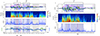 |
Fig. 2. Trace PSD of magnetic field fluctuation, PB, in the inertial MHD range and fluctuation amplitude |δB|/B from Wind and STA observations and transverse velocity components, Vy, z, obtained from the Wind observation. The horizontal lines in the Vy, z panel indicate Vy, z = 50 km/s. The hatched regions indicate the intervals of ejecta cores. The black and red vertical lines indicate the shock resulting from the arrival of complex solar wind structures and REs (discussed in Section 3.4), respectively. |
In the last row of Figure 2a, we provide the transverse solar wind velocity Vy (in green) and Vz (in blue). We located two highly sheared regions with a duration of more than an hour with non-radial velocity components Vy > 50 and Vz > 50 km/s within W1 and W2, respectively. The first sheared region is associated with a shock within W1, noted by Weiler et al. (2025). A non-radial velocity component may present at a sheath region following an interplanetary shock and can also manifest Alfvénic fluctuations resulting from interaction among field lines (Scolini et al. 2025). Furthermore, expansion of the ejecta may lead to the development of non-radial flow within the structures (Al-Haddad et al. 2022). However, signatures of over-expansion were not noted during the W1 and W2 intervals.
The solar wind following W2 shows signatures of an individual ejecta interval evident from low intensity of PB and |δB|, Na/Np > 0.08, an decrease in Np and β < 0.1, and Tp < Tex. This ejecta does not contain tightly wound magnetic field lines as indicated by the behavior of magnetic field vectors and the absence of a localized helical region in the Hm spectrum during the interval. Such characteristics can arise when a spacecraft crosses through an ejecta leg.
3.4. Reconnection exhausts within complex intervals
From the previous sections, it is clear that the complex intervals W1, W2, and S1 are formed of multiple ejecta. Therefore, in this section, we look for the presence of reconnection exhausts (REs) within the complex intervals where the ejecta cores are not present. We transformed Bx, y, z, Vx, y, z from GSE to the LMN coordinate (BLMN, VLMN) system where L, M, and N indicate the maximum, intermediate, and minimum variance directions and are obtained by minimum variance analysis (MVA; Sonnerup & Cahill 1968; Gosling & Phan 2013). In this coordinate system, L is assumed to point toward the reconnection outflow, M along the reconnection X-line, and N is toward the normal direction of the reconnection current sheet (Phan et al. 2006). We used suprathermal electron PAD; the ion energy spectrum, IE, in the 500–5000 eV range; and Np and Tp measurements to identify REs because field line connectivity at REs may lead isotropic or bi-directional PAD (Gosling 2009) and energy conversion to other forms during reconnection may intensify IE, Np, and Tp. In Figure 3, we show intervals of REs in red and indicate them in Figures 1 and 2 using red dotted vertical lines.
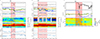 |
Fig. 3. Solar wind magnetic and plasma embedding RE intervals RE1, RE2, and RE3 (in red) observed by the MAG, SWE, and 3DP instruments on board Wind (a, b) and the MAG and SWEA instruments on board STA/IMPACT (c). We note that in panels a and b, the VL, M, N has been rescaled for clarity. |
In the Wind observation, we located two REs, one within W1 and another between W1 and W2, where B decreases, BL changes direction, |VL| has an elevated value due to reconnection outflow, Np and Tp show enhancement, PAD becomes isotropic, and IE shows enhanced flux abundance. The limited coverage, lack of plasma velocity vectors, and low resolution of plasma data from STA made it difficult to locate REs within S1. Using only B, BLMN, electron PAD, and low-resolution Np and Tp measurements from STA, we confidently located only one RE within S1 and show its characteristics in Figure 3c. This RE is formed between the last two ejecta cores within S1. Nevertheless, S1 may contain more REs that are difficult to identify due to the STA data quality.
3.5. Complex intervals in the heliospheric imagers
We further investigated the presence of multiple ICMEs in the complex intervals W1, W2, and S1 using the heliospheric imagers H1 and H2 on board STA. In the right panel of Figure 4, we provide a time-elongation (ϵ) map (J-map) formed of stacked running-difference images of STA/HI1 and HI2 during May 8-13, 2024, within a slit along the ecliptic plane. At 20° < ϵ < 60° in the J-map, we identified a large bright feature formed of multiple CME leading edges. We tracked the leading (in blue symbol) and trailing (in red symbol) edges of the bright feature shown until ϵ = 60° (left panel on Figure 4) and fit them using the HM technique to derive their arrivals at the Wind spacecraft located at ϵ ∼ 98°. Our estimated arrival of the leading and trailing edges of the large bright feature was within 16 and 10 minutes of the observed start and end times of W1 and W2, respectively.
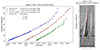 |
Fig. 4. Left panel: Elongation angle vs. time for the three tracked structures on May 8-10: Beginning of W1 (blue diamonds), end of W2 (red diamonds), and CME6 leading edge (green diamonds). The black continuous line denotes the best HM fit for the three structures. Predicted arrivals to Earth and fitting residues are presented in the figure. Right panel: Jmap at a position angle of 90° for a combination of COR2, HI1, and HI2 on board STEREO-A. Dashed lines represent the mentioned tracked structures: W1, W2, and CME6 respectively in light blue, red, and green. |
While tracking the large bright feature down to the solar origin up to ϵ = 2.5°, we found its association with CMEs (CME1-CME5 in Table 1) originating on May 8, including the filament-associated CME3. Another separate bright front observed in the J-map, marked in green, could be unambiguously tracked up to ϵ = 36°. This track could be associated with the CME6 in Table 1, which originated early on May 9 and had a speed higher than the previous CMEs. In the J-map, the leading edge of CME6 (in green) has been extrapolated until the Earth’s location using the HM technique. It is estimated to have arrived at Wind ∼20 minutes after the observed start time of the ejecta, which corresponds to the last hatched interval in Figures 1 and 2, with a speed higher than the preceding events.
4. Discussion and conclusion
The analysis performed in this study of the complex solar wind interval featuring multiple ICMEs on May 10-11, 2024, reveals notable differences between two heliospheric locations separated by ∼12° in longitude and 1.5° in latitude. At Wind, the total magnetic energy and helicity within the 0.5–64 hour scale range were found to be 60% and 35% of those measured at STA, respectively. Therefore, had part of the complex ICME structure encountered by STA hit the Earth instead, it could have caused a geomagnetic storm even more intense than was observed in the actual scenario. However, for a given amount of solar wind energy, the resulting geomagnetic disturbance may vary substantially, as the solar wind-magnetosphere coupling depends on several factors apart from solar wind energy, such as solar wind speed and density, the transverse component of solar wind magnetic field, clock angle (Lockwood 2022), preconditioning of the magnetosphere, and presence of solar wind structures. ICMEs represent the most energetic and geoeffective driver (Telloni et al. 2020a). The probable reason behind the significant difference in magnetic content of the Wind and STA counterparts despite the moderate longitudinal separation of the observing spacecraft is discussed below.
The regions W1 and S1′ contain a complex, merged, and highly helical structure with enhanced magnetic energy resulting from the merging of ejecta associated with CME1 and CME2, where the merging process is further evident at the smaller scales in the helicity spectrum. The high magnetic energy is associated with the larger fluctuations in magnetic field lines in the larger-scale sizes corresponding to the injection range of MHD frequency. The two CMEs originated from the same solar source but approximately 7 hours apart and carried right-handed magnetic field lines. Their flux rope types derived from field line rotational directions and axial tilt mentioned in Table 1 indicate that their handedness and axial orientations favor magnetic reconnection that might have initiated at their early propagation. The evidence for ongoing reconnection is even found from the presence of an RE (RE1) within W1 between the first two ejecta cores, ‘WC1’ and ‘WC2’.
When fitting the linear force-free flux rope model (Lepping et al. 1990) to three ejecta cores (hatched intervals) within W2, we found that the side structures exhibited right-handed helicity, while the central one displayed left-handed helicity. The inclination angles of the flux ropes were θ = −7°, −14°, and −13°, and the azimuthal angle was ϕ = 308°, 176°, and 5°, respectively. This indicates that W2 includes the flank of a left-handed ejecta originating from the filament associated CME3 that propagated at least 27° eastward from the Sun-Earth line (Weiler et al. 2025). This ejecta core, ‘WC3’, was bound by two right-handed ejecta cores, ‘WC4’ and ‘WC5’, which is in line with the investigation by Weiler et al. (2025). Using J-map and the ELliptical Evolution model (Möstl et al. 2015), Weiler et al. (2025) concluded that CME3 was being overtaken by the following right-handed CME4 sourcing ‘WC4’ that arrived earlier than ‘WC3’ at Wind spacecraft. The CME3 and CME4 may not have magnetically reconnected because of their unfavorable orientation (opposite handedness with non anti-parallel axes). Also, the Hm map indicates that ‘WC4’ and ‘WC3’ may not reconnect, as they correspond to Hm > 0 and Hm < 0 in the away magnetic field sector, indicating anti-clockwise and clockwise rotations, respectively. In the Wind in situ observation, a sheared region with Vz > 50 km/s and comparatively higher Na/Np, Np, β, and PB appeared between “WC4” and “WC3”, and it indicates a sheath-like structure. The opposite handedness and almost anti-parallel axial orientations (with an axial separation of ∼171°) of ‘WC3’ and ‘WC5’ within W2 favors magnetic reconnection. This interpretation is further evidenced by the intensified electron PAD at two opposite directions. However, the CME5 sourcing ‘WC5’ propagated far westward from the CME3 propagation direction with a separation angle of ∼65°. The CME5 and CME6 had an initial propagation direction ∼38° and ∼27° westward from the Sun-Earth line, respectively. Therefore, it was hard to track these CMEs at a higher elongation angle in the J-map, which was prepared at a position angle of 90°.
Except for the left-handed CME3, which propagated much more eastward (∼40°) of STA and was far from reaching its location, all other CMEs were westward of the Sun-Earth line and had a high speed, therefore, had a more head-on impact on the STA. All right-handed ICMEs associated with the same polarity inversion line belonging to the bottom part of the AR13664 (Wang et al. 2024) had almost parallel axial orientations. They magnetically reconnected and merged to form a large-complex ejecta. In contrast to the Wind observation, at STA, it was hard to individually associate the ejecta cores with their progenitor CMEs. The complex ejecta appeared with a characteristic core size exceeding ΔS > 7 h and strong helical field lines with σm = 0.9 at STA.
A detailed study of the solar wind energy-Dst distribution performed by Telloni et al. (2020a) demonstrated a robust correlation between the amount of energy stored in the solar wind interacting with the Earth’s magnetosphere and the intensity of the induced geomagnetic disturbance. To explore the scatter in Dst for a fixed energy input, contributions of the solar wind bulk speed and Bz intensity were analyzed in the energy-Dst space. This implies that slow solar wind has a negligible effect on Earth regardless of its energy content, and solar wind with low and mid energies may induce geomagnetic disturbances by long duration and strong southward Bz driving magnetic reconnection between the solar wind and magnetosphere. Moreover, high-energy and high-speed solar events can result in severe geomagnetic disturbances irrespective of their field line orientations. The STA’s limitation in plasma measurements generate caveats in detailed assessments of solar wind-magnetosphere coupling factors of the STA counterpart. The initial propagation properties inferred from the coronagraph and HI analysis in combination with the solar wind in situ magnetic measurement analysis indicate an arrival of a high-speed, high-energy complex solar wind interval carrying multiple interacting ICME ejecta, which further conforms with the hypothesis that the STA counterpart had a higher geoeffectivity than that of the Wind counterpart. However, in a complex solar wind scenario, the hypothesis of a comparatively high energetic solar wind driving a larger geomagnetic response needs to be further investigated considering the influence of other coupling factors; thus it calls for numerical MHD-driven magnetospheric simulations and statistical studies across multiple interacting ICME ejecta.
In this study, we have investigated the in situ magnetic and plasma properties of a complex solar wind interval during May 10-11, 2024, when one of the strongest recorded geomagnetic storms occurred. Our goal was to understand its formation and study its magnetic content that made it capable of driving such a huge storm. With the use of plasma properties and magnetic field fluctuation analysis in the inertial range of frequency, we located six (five) ICME ejecta cores within the complex interval counterparts hitting the Wind (STA) spacecraft. By analyzing the solar wind magnetic field in the time-frequency domain across a large range of frequencies, we quantified the magnetic helicity and energy, and the helical core scale-size of the complex ejecta at the Wind and STA counterparts and found the reason for their substantial differences even with a moderate angular separation of 12° (0.04 au) in the heliosphere. We attribute these differences primarily to the complicated interaction among ejecta at the Wind counterpart, where a left-handed ejecta appeared between two right-handed common-origin ejecta with a non-favorable orientation for strong reconnection. In the STA counterpart, ejecta strongly reconnected due to all of them having right-handed rotations and parallel axial orientations and a common origin.
Acknowledgments
We acknowledge the data source Goddard Space Flight Center’s Space Physics Data Facility (SPDF) from where we downloaded the in situ solar wind data and use of JHelioviewer. We thank Wind and STEREO mission teams for making the data publicly available. S.P is thankful for the support of NASA Postdoctoral Program fellowship, L.K.J. thanks for the support of the STEREO mission and Heliophysics Guest Investigator Grant 80NSSC23K0447. T.N-C. thanks for the support of the Solar Orbiter and Parker Solar Probe missions, Heliophysics Guest Investigator Grant 80NSSC23K0447 and the GSFC-Heliophysics Innovation Funds. Y. acknowledge support by NSF grant AGS-2300961 and NASA grant 80NSSC24K0724.
References
- Acuña, M. H., Curtis, D., Scheifele, J. L., et al. 2008, Space Sci. Rev., 136, 203 [Google Scholar]
- Alberti, T., Narita, Y., Hadid, L. Z., et al. 2022, A&A, 664, L8 [NASA ADS] [CrossRef] [EDP Sciences] [Google Scholar]
- Al-Haddad, N., & Lugaz, N. 2025, Space Sci. Rev., 221, 12 [Google Scholar]
- Al-Haddad, N., Galvin, A. B., Lugaz, N., Farrugia, C. J., & Yu, W. 2022, ApJ, 927, 68 [NASA ADS] [CrossRef] [Google Scholar]
- Ang, D. J., Buhari, S. M., Abdullah, M., & Bahari, S. A. 2025, J. Geophys. Res. (Space Phys.), 130, e2024JA033601 [Google Scholar]
- Baruah, Y., Roy, S., Sinha, S., et al. 2024, Space Weather, 22, e2023SW003716 [Google Scholar]
- Batchelor, G. K. 1953, The Theory of Homogeneous Turbulence (Cambridge: Cambridge University Press) [Google Scholar]
- Bosman, E., Bothmer, V., Nisticò, G., et al. 2012, Sol. Phys., 281, 167 [NASA ADS] [Google Scholar]
- Braga, C. R., Vourlidas, A., Liewer, P. C., et al. 2022, ApJ, 938, 13 [NASA ADS] [CrossRef] [Google Scholar]
- Bruno, R., & Dobrowolny, M. 1986, Ann. Geophys., 4, 17 [NASA ADS] [Google Scholar]
- Burton, R. K., McPherron, R. L., & Russell, C. T. 1975, J. Geophys. Res., 80, 4204 [NASA ADS] [CrossRef] [Google Scholar]
- Chen, C. H. K., Bale, S. D., Bonnell, J. W., et al. 2020, ApJS, 246, 53 [Google Scholar]
- Clilverd, M. A., Rodger, C. J., Manus, D. H. M., et al. 2025, Space Weather, 23, e2024SW004235 [Google Scholar]
- Díaz, J. 2025, Sci. Rep., 15, 5922 [Google Scholar]
- Farrugia, C. J., Jordanova, V. K., Thomsen, M. F., et al. 2006a, J. Geophys. Res. (Space Phys.), 111, A11104 [Google Scholar]
- Farrugia, C. J., Matsui, H., Kucharek, H., et al. 2006b, Adv. Space Res., 38, 498 [Google Scholar]
- Freeland, S. L., & Handy, B. N. 1998, Sol. Phys., 182, 497 [Google Scholar]
- Galvin, A. B., Kistler, L. M., Popecki, M. A., et al. 2008, Space Sci. Rev., 136, 437 [Google Scholar]
- Gonzalez, W. D., Echer, E., Clúa de Gonzalez, A. L., Tsurutani, B. T., & Lakhina, G. S. 2011, J. Atmosph. Sol.-Terr. Phys., 73, 1447 [Google Scholar]
- Good, S. W., Rantala, O. K., Jylhä, A. S. M., et al. 2023, ApJ, 956, L30 [Google Scholar]
- Gosling, J. T. 2009, in Universal Heliophysical Processes, eds. N. Gopalswamy, & D. F. Webb, IAU Symp., 257, 367 [Google Scholar]
- Gosling, J. T., & Phan, T. D. 2013, ApJ, 763, L39 [Google Scholar]
- Hayakawa, H., Ebihara, Y., Mishev, A., et al. 2025, ApJ, 979, 49 [Google Scholar]
- Howard, R. A., Moses, J. D., Vourlidas, A., et al. 2008, Space Sci. Rev., 136, 67 [NASA ADS] [CrossRef] [Google Scholar]
- Jaswal, P., Sinha, S., & Nandy, D. 2025, ApJ, 979, 31 [Google Scholar]
- Kay, C., Mays, M. L., & Collado-Vega, Y. M. 2022, Space Weather, 20, e2021SW002914 [NASA ADS] [Google Scholar]
- Khuntia, S., Mishra, W., & Agarwal, A. 2025, A&A, 698, A79 [NASA ADS] [CrossRef] [EDP Sciences] [Google Scholar]
- Kilpua, E., Koskinen, H. E. J., & Pulkkinen, T. I. 2017, Liv. Rev. Sol. Phys., 14, 5 [Google Scholar]
- Kilpua, E. K. J., Good, S. W., Ala-Lahti, M., et al. 2021, Front. Astron. Space Sci., 7, 109 [CrossRef] [Google Scholar]
- Klein, L. W., & Burlaga, L. F. 1982, J. Geophys. Res., 87, 613 [Google Scholar]
- Kwak, Y.-S., Kim, J.-H., Kim, S., et al. 2024, J. Astron. Space Sci., 41, 171 [Google Scholar]
- Lepping, R. P., Jones, J. A., & Burlaga, L. F. 1990, J. Geophys. Res., 95, 11957 [Google Scholar]
- Lepping, R. P., Acũna, M. H., Burlaga, L. F., et al. 1995, Space Sci. Rev., 71, 207 [Google Scholar]
- Lin, R. P., Anderson, K. A., Ashford, S., et al. 1995, Space Sci. Rev., 71, 125 [CrossRef] [Google Scholar]
- Liu, Y. D., Luhmann, J. G., Kajdič, P., et al. 2014, Nat. Commun., 5, 3481 [NASA ADS] [Google Scholar]
- Liu, Y. D., Hu, H., Zhao, X., Chen, C., & Wang, R. 2024, ApJ, 974, L8 [NASA ADS] [CrossRef] [Google Scholar]
- Lockwood, M. 2022, Space Weather, 20, e2021SW002989 [CrossRef] [Google Scholar]
- Lopez, R. E. 1987, J. Geophys. Res., 92, 11189 [Google Scholar]
- Lugaz, N. 2010, Sol. Phys., 267, 411 [NASA ADS] [CrossRef] [Google Scholar]
- Lugaz, N., Manchester, W. B., IV, & Gombosi, T. I. 2005, ApJ, 634, 651 [NASA ADS] [CrossRef] [Google Scholar]
- Lugaz, N., Vourlidas, A., & Roussev, I. I. 2009, Ann. Geophys., 27, 3479 [Google Scholar]
- Lugaz, N., Farrugia, C. J., Manchester, W. B., IV, & Schwadron, N. 2013, ApJ, 778, 20 [NASA ADS] [CrossRef] [Google Scholar]
- Lugaz, N., Al-Haddad, N., Zhuang, B., et al. 2025, Space Weather, 23, 2024SW004189 [Google Scholar]
- Luhmann, J. G., Gopalswamy, N., Jian, L. K., & Lugaz, N. 2020, Sol. Phys., 295, 61 [NASA ADS] [CrossRef] [Google Scholar]
- Manchester, W., Kilpua, E. K. J., Liu, Y. D., et al. 2017, Space Sci. Rev., 212, 1159 [Google Scholar]
- Martin, S. F. 1998, Sol. Phys., 182, 107 [Google Scholar]
- Matthaeus, W. H., & Goldstein, M. L. 1982, J. Geophys. Res., 87, 6011 [Google Scholar]
- Mayank, P., Lotz, S., Vaidya, B., Mishra, W., & Chakrabarty, D. 2024, ApJ, 976, 126 [Google Scholar]
- Moffatt, H. K. 1978, Magnetic Field Generation in Electrically Conducting Fluids (Cambridge: University Press) [Google Scholar]
- Montgomery, D., & Turner, L. 1981, Phys. Fluids, 24, 825 [Google Scholar]
- Möstl, C., Rollett, T., Lugaz, N., et al. 2011, ApJ, 741, 34 [CrossRef] [Google Scholar]
- Möstl, C., Rollett, T., Frahm, R. A., et al. 2015, Nat. Commun., 6, 7135 [CrossRef] [Google Scholar]
- Nandy, D., Baruah, Y., Bhowmik, P., et al. 2023, J. Atmosph. Sol.-Terr. Phys., 248, 106081 [Google Scholar]
- Narock, T., Pal, S., Arsham, A., Narock, A., & Nieves-Chinchilla, T. 2024, Sol. Phys., 299, 131 [Google Scholar]
- Nieves-Chinchilla, T., Pal, S., Salman, T. M., et al. 2023, Front. Astron. Space Sci., 10, 56 [Google Scholar]
- O’Brien, T. P., & McPherron, R. L. 2000, J. Geophys. Res., 105, 7707 [CrossRef] [Google Scholar]
- Ogilvie, K. W., Chornay, D. J., Fritzenreiter, R. J., et al. 1995, Space Sci. Rev., 71, 55 [Google Scholar]
- Oliveira, D. M., Zesta, E., & Garcia-Sage, K. 2025, Front. Astron. Space Sci., 12-2025 [Google Scholar]
- Owens, M. J., Spence, H. E., McGregor, S., et al. 2008, Space Weather, 6, S08001 [Google Scholar]
- Pal, S., Gopalswamy, N., Nandy, D., et al. 2017, ApJ, 851, 123 [Google Scholar]
- Pal, S., Dash, S., & Nandy, D. 2020, Geophys. Res. Lett., 47, e86372 [Google Scholar]
- Pal, S., Kilpua, E., Good, S., Pomoell, J., & Price, D. J. 2021, A&A, 650, A176 [NASA ADS] [CrossRef] [EDP Sciences] [Google Scholar]
- Pal, S., Lynch, B. J., Good, S. W., et al. 2022a, Front. Astron. Space Sci., 9, 903676 [NASA ADS] [CrossRef] [Google Scholar]
- Pal, S., Nandy, D., & Kilpua, E. K. J. 2022b, A&A, 665, A110 [NASA ADS] [CrossRef] [EDP Sciences] [Google Scholar]
- Pal, S., Balmaceda, L., Weiss, A. J., et al. 2023, Front. Astron. Space Sci., 10, 1195805 [Google Scholar]
- Pal, S., dos Santos, L. F. G., Weiss, A. J., et al. 2024, ApJ, 972, 94 [Google Scholar]
- Palmerio, E., Kay, C., Al-Haddad, N., et al. 2021, ApJ, 920, 65 [NASA ADS] [CrossRef] [Google Scholar]
- Palmerio, E., Carcaboso, F., Khoo, L. Y., et al. 2024, ApJ, 963, 108 [NASA ADS] [CrossRef] [Google Scholar]
- Phan, T. D., Gosling, J. T., Davis, M. S., et al. 2006, Nature, 439, 175 [Google Scholar]
- Rüdisser, H. T., Nguyen, G., Le Louëdec, J., & Möstl, C. 2025, arXiv e-prints [arXiv:2505.09365] [Google Scholar]
- Sarkar, R., Gopalswamy, N., & Srivastava, N. 2020, ApJ, 888, 121 [NASA ADS] [CrossRef] [Google Scholar]
- Schmidt, J., & Cargill, P. 2004, Ann. Geophys., 22, 2245 [Google Scholar]
- Scolini, C., Zhuang, B., Lugaz, N., et al. 2025, ApJ, 978, 146 [Google Scholar]
- Shen, F., Wu, S. T., Feng, X., & Wu, C.-C. 2012, J. Geophys. Res. (Space Phys.), 117, A11101 [Google Scholar]
- Sonnerup, B. U. Ö., & Cahill, L. J., Jr 1968, J. Geophys. Res., 73, 1757 [Google Scholar]
- Takahashi, T., & Shibata, K. 2017, ApJ, 837, L17 [NASA ADS] [CrossRef] [Google Scholar]
- Telloni, D., Bruno, R., D’Amicis, R., Pietropaolo, E., & Carbone, V. 2012, ApJ, 751, 19 [Google Scholar]
- Telloni, D., Perri, S., Bruno, R., Carbone, V., & Amicis, R. D. 2013, ApJ, 776, 3 [Google Scholar]
- Telloni, D., Carbone, V., Perri, S., et al. 2016, ApJ, 826, 205 [Google Scholar]
- Telloni, D., Antonucci, E., Bemporad, A., et al. 2019, ApJ, 885, 120 [Google Scholar]
- Telloni, D., Carbone, F., Antonucci, E., et al. 2020a, ApJ, 896, 149 [NASA ADS] [CrossRef] [Google Scholar]
- Telloni, D., Zhao, L., Zank, G. P., et al. 2020b, ApJ, 905, L12 [NASA ADS] [CrossRef] [Google Scholar]
- Telloni, D., Scolini, C., Möstl, C., et al. 2021, A&A, 656, A5 [NASA ADS] [CrossRef] [EDP Sciences] [Google Scholar]
- Telloni, D., Schiavo, M. L., Magli, E., et al. 2023, ApJ, 952, 111 [NASA ADS] [CrossRef] [Google Scholar]
- Thampi, S. V., Bhaskar, A., Mayank, P., Vaidya, B., & Venugopal, I. 2025, ApJ, 981, 76 [Google Scholar]
- Thernisien, A. 2011, ApJS, 194, 33 [Google Scholar]
- Thernisien, A. F. R., Howard, R. A., & Vourlidas, A. 2006, ApJ, 652, 763 [Google Scholar]
- Tulasi Ram, S., Veenadhari, B., Dimri, A. P., et al. 2024, Space Weather, 22, 2024SW004126 [Google Scholar]
- Wan, Q., Ma, G., Zhou, G., Li, J., & Fan, J. 2025, J. Geophys. Res. (Space Phys.), 130, e2024JA033627 [Google Scholar]
- Wang, Y. M., Ye, P. Z., Wang, S., & Xue, X. H. 2003, Geophys. Res. Lett., 30, 1700 [Google Scholar]
- Wang, R., Liu, Y. D., Zhao, X., & Hu, H. 2024, A&A, 692, A112 [NASA ADS] [CrossRef] [EDP Sciences] [Google Scholar]
- Weiler, E., Möstl, C., Davies, E. E., et al. 2025, Space Weather, 23, 2024SW004260 [Google Scholar]
- Weiss, A. J., Nieves-Chinchilla, T., & Möstl, C. 2024, ApJ, 975, 169 [Google Scholar]
- Xie, H., Gopalswamy, N., Manoharan, P. K., et al. 2006, J. Geophys. Res. (Space Phys.), 111, A01103 [Google Scholar]
- Yogesh, Chakrabarty, D., & Srivastava, N. 2022, MNRAS, 513, L106 [Google Scholar]
- Zakharenkova, I., Cherniak, I., Braun, J. J., et al. 2025, Space Weather, 23, e2024SW004245 [Google Scholar]
- Zhang, M., Feng, X., Li, H., et al. 2023, Front. Astron. Space Sci., 10, 1105797 [Google Scholar]
- Zhang, X., Xie, T., Ye, Q., Yan, L., & Wu, X. 2025a, Geophys. Res. Lett., 52, e2025GL115104 [Google Scholar]
- Zhang, Z., Zhang, F., Wang, L., et al. 2025b, Space Weather, 23, e2024SW004197 [Google Scholar]
- Zhao, L. L., Zank, G. P., Adhikari, L., et al. 2020, ApJS, 246, 26 [Google Scholar]
- Zhao, L. L., Zank, G. P., Hu, Q., et al. 2021, A&A, 650, A12 [NASA ADS] [CrossRef] [EDP Sciences] [Google Scholar]
All Tables
All Figures
|
Fig. 1. In situ observation during May 10-11, 2024, using (a) MAG and SWE instruments on board Wind and (b) MAG, SWEA, and PLASTIC instruments on board the STA spacecraft. The dotted lines in the ϕ panel indicate the nominal sector boundaries of the interplanetary magnetic field derived using a Parker spiral angle obtained from the local solar wind observations at Wind and STA. Here, ϕ values between (outside) the lines indicate the magnetic field in the away (toward) sector of the heliosphere. The blue shaded regions of W1, W2, and S1 present the localized helicity regions in both the time and frequency domains (see Section 3.2 for details). The hatched intervals indicate an unperturbed core of ejecta, as discussed in Section 3.3. The eighth (seventh) column in panel a (b) shows the energy flux (phase space density) of suprathermal electrons in the 265 (247) eV energy bin. |
| In the text | |
|
Fig. 2. Trace PSD of magnetic field fluctuation, PB, in the inertial MHD range and fluctuation amplitude |δB|/B from Wind and STA observations and transverse velocity components, Vy, z, obtained from the Wind observation. The horizontal lines in the Vy, z panel indicate Vy, z = 50 km/s. The hatched regions indicate the intervals of ejecta cores. The black and red vertical lines indicate the shock resulting from the arrival of complex solar wind structures and REs (discussed in Section 3.4), respectively. |
| In the text | |
|
Fig. 3. Solar wind magnetic and plasma embedding RE intervals RE1, RE2, and RE3 (in red) observed by the MAG, SWE, and 3DP instruments on board Wind (a, b) and the MAG and SWEA instruments on board STA/IMPACT (c). We note that in panels a and b, the VL, M, N has been rescaled for clarity. |
| In the text | |
|
Fig. 4. Left panel: Elongation angle vs. time for the three tracked structures on May 8-10: Beginning of W1 (blue diamonds), end of W2 (red diamonds), and CME6 leading edge (green diamonds). The black continuous line denotes the best HM fit for the three structures. Predicted arrivals to Earth and fitting residues are presented in the figure. Right panel: Jmap at a position angle of 90° for a combination of COR2, HI1, and HI2 on board STEREO-A. Dashed lines represent the mentioned tracked structures: W1, W2, and CME6 respectively in light blue, red, and green. |
| In the text | |
Current usage metrics show cumulative count of Article Views (full-text article views including HTML views, PDF and ePub downloads, according to the available data) and Abstracts Views on Vision4Press platform.
Data correspond to usage on the plateform after 2015. The current usage metrics is available 48-96 hours after online publication and is updated daily on week days.
Initial download of the metrics may take a while.