© The Authors 2025

1. Introduction

Binary neutron star (BNS) mergers are one of the main sources of gravitational waves (GWs) in the frequency range of sensitivity of the current ground-based GW detectors, such as the two detectors in the Advanced Laser Interferometer Gravitational wave Observatory (LIGO, LIGO Scientific Collaboration 2015), the Advanced Virgo (Acernese et al. 2015) detector, and the KAGRA (Somiya 2012) detector. These sources are of particular interest because of their multi-messenger nature: in addition to GWs emitted during the inspiral, merger, and post-merger phases, BNS coalescences also produce kilonovae (Li & Paczyński 1998; Metzger 2020) and non-thermal emission related to the launch of a relativistic jet (e.g. Eichler et al. 1989; Lazzati et al. 2017; Nakar 2020). As was demonstrated by the spectacular GW170817 event (Abbott et al. 2017a,b; Margutti & Chornock 2021), observations of these multiple messengers can have a tremendous impact on several branches of physics, including fundamental physics (e.g. Abbott et al. 2019; Baker et al. 2017; Creminelli & Vernizzi 2017), nuclear physics (e.g. Abbott et al. 2018a), cosmology (e.g. Abbott et al. 2017c), the synthesis of heavy elements (e.g. Coulter et al. 2017; Pian et al. 2017; Kasen et al. 2017; Kajino et al. 2019), the physics of gamma-ray bursts and their jets (e.g. Abbott et al. 2017d; Savchenko et al. 2017; Kasliwal et al. 2017; Mooley et al. 2018; Ghirlanda et al. 2019), and massive binary stellar evolution (e.g. Kruckow et al. 2018; Mapelli & Giacobbo 2018), to name only a few.

The transformative potential of multi-messenger observations of these sources must confront with the very challenging nature of their electromagnetic follow-up, due to the faintness of the electromagnetic emission combined with the poor GW localization (see e.g. Nicholl & Andreoni 2025). In the last several years, the international transient astronomy community has made a large effort to be ready to take on this challenge. Such organizational effort, which includes allocating human resources and applying for observing time at the best astronomical facilities worldwide, is guided by, and gauged on, predictions of the expected detection rate of such events. Most such predictions for the current observing run, O4, of the LIGO-Virgo-KAGRA (LVK) network have proven to be rather optimistic (see Colombo et al. 2022, who provide a convenient summary of many predictions from the literature in their discussion section), and even the official LVK predictions (available on the LVK Public Alerts User Guide web page¹ and based on Petrov et al. 2022) have promised tens of BNS merger public alerts to be delivered by the GW detector network during O4.

In this work, I present a method of calculating the probability of future BNS (and neutron star–black hole, NSBH) merger detections by the LVK network that is independent of the uncertain mass distribution of the merging binaries, and that uses only the information on the past number of detections, combined with an estimate of the ratio between the sensitivity of the target run with respect to the previous runs that requires only publicly available information as an input. Using this method, I provide updated predictions for the probability of one or more BNS and NSBH detections in the remainder of O4, and in the next observing run, O5.

2. Poisson probability informed by previous occurrences of a rare event

I derive here the expression that I used in order to forecast the probability of detecting GWs from new BNS and BHNS events in future observing runs. After carrying out the derivation, I was informed that it is essentially identical to that presented in Appendix B of Ray et al. (2023), and that the result coincides with Eq. (42) in Essick (2023) in a particular case.

Let N be the a number of occurrences of a rare event over a period of time, T, and let λ be the expected number of events; that is, the average occurrence rate multiplied by T. The probability of N given λ is the Poisson probability

$$\begin{array}{c}\hfill p(N|\lambda )=\frac{{\lambda }^{N}exp(-\lambda )}{N!}·\end{array}$$(1)

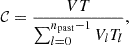
Now let N′ be a number of previously observed events over a different time period, T′, over which the expected number of events was λ′, with 𝒞 = λ/λ′. The posterior probability of λ′ given N′ can be written through Bayes’ theorem as

$$\begin{array}{c}\hfill p(\lambda \prime |N^{\prime })=\frac{p(N^{\prime }|\lambda \prime )\pi (\lambda \prime )}{p(N^{\prime })}=\frac{{{\lambda }^{\prime }}^{N^{\prime }}exp(-\lambda \prime )}{N^{\prime }!}\frac{\pi (\lambda \prime )}{p(N^{\prime })},\end{array}$$(2)

where π(λ′) is the prior probability of λ′. We opt to parametrize this as

$$\begin{array}{c}\hfill \pi (\lambda \prime )=\left(\frac{p(N^{\prime })N^{\prime }!}{\mathrm{\Gamma }(N^{\prime }+1-\alpha )}\right){\lambda }^{-\alpha },\end{array}$$(3)

where Γ(x) is the Gamma function and the factor in parentheses ensures the correct normalization of the posterior. With this definition, α = 0 corresponds to a uniform prior, α = 1/2 to the Jeffreys prior for the Poisson probability scale parameter, and α = 1 to a prior that is uniform in the logarithm. Since these are the most common choices for an uninformative prior on this parameter, I limit the discussion here to these cases.

The above definitions allowed us to derive the posterior probability on N given the previously observed number of events, N′, as follows. The starting point was

$$\begin{array}{cc}\hfill p(N|N^{\prime })& ={\displaystyle \int p}(N|\lambda )p(\lambda |N^{\prime })\mathrm{d}\lambda \hfill \\ \hfill & ={\displaystyle \int p}(N|\lambda ){\displaystyle \int p}(\lambda |\lambda \prime )p(\lambda \prime |N^{\prime })\mathrm{d}\lambda \prime \mathrm{d}\lambda .\hfill \end{array}$$(4)

Noting that p(λ | λ′) = δ(λ − 𝒞λ′), where δ is the Dirac delta, this led to

$$\begin{array}{c}\hfill p(N|N^{\prime })=\frac{{\mathcal{C}}^{\alpha -N^{\prime }-1}}{\mathrm{\Gamma }(N^{\prime }+1-\alpha )}{\displaystyle \int p}(N|\lambda )exp(-\frac{\lambda }{\mathcal{C}}){\lambda }^{N^{\prime }-\alpha }\mathrm{d}\lambda .\end{array}$$(5)

Substituting Eq. (1) in the above expression, carrying out the integral, and using N!=Γ(N + 1), we arrived at

$$\begin{array}{c}\hfill p(N|N^{\prime },\alpha ,\mathcal{C})=\frac{\mathrm{\Gamma }(N+N^{\prime }+1-\alpha )}{\mathrm{\Gamma }(N+1)\mathrm{\Gamma }(N^{\prime }+1-\alpha )}\frac{{\mathcal{C}}^N}{{(1+\mathcal{C})}^{N+N^{\prime }+1-\alpha }},\end{array}$$(6)

where the dependency on the prior index, α, and the expected number ratio, 𝒞, has been made explicit.

3. Application to compact binary mergers

If the sensitivity range of the GW detector network to the sources under consideration does not extend to large redshifts, the cosmic evolution of the population and cosmological effects can be neglected, so that the expected number of detections over an observing run of duration T can be expressed simply as λ = R₀VT, where R₀ is the local rate density of compact binary mergers and V is the effective volume over which the network is sensitive to such sources. In this context, the ratio λ/λ′ is then simply the ratio of the effective sensitive time volume of the run to that of past runs; namely,

$$\begin{array}{c}\hfill \mathcal{C}=\frac{\mathit{VT}}{{\displaystyle {\sum }_{l=0}^{n_{\mathrm{past}}-1}}{V}_l{T}_l},\end{array}$$(7)

where l runs over past observing runs, whose total number is n_past. In the following, I describe a strategy to estimate such a ratio using basic information such as the BNS ranges and duty cycles of the detectors.

3.1. Evaluation of the effective sensitive volume for each run

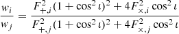
The ‘optimal’ matched filter signal-to-noise ratio (S/N) of a single merger, ρ_opt, assuming it to be dominated by the inspiral part of the signal, depends on the chirp mass, m_c = (m₁m₂)^3/5/(m₁ + m₂)^1/5 (where m₁ and m₂ are the gravitational masses of the primary and secondary components of the binary, respectively), the luminosity distance, r, and the detector noise power spectral density curve, 𝒮(f), as a function of the frequency, f, through the integral²f_7/3 = ∫[f^7/3𝒮(f)]⁻¹df (Finn & Chernoff 1993), so that

$$\begin{array}{c}\hfill {\rho }_{\mathrm{opt}}\propto \frac{m_{\mathrm{c}}^{5/6}}{r}{f}_{7/3}.\end{array}$$(8)

The actual S/N in a given detector, which I indicate with the symbol ρ, also depends on the source position in the detector’s sky (defined e.g. by a pair of spherical angular co-ordinates θ, ϕ), its inclination, ι, with respect to the line of sight, and its polarization angle, ψ, all of which can be summarized into a single parameter, 0 ≤ w ≤ 1, such that ρ = wρ_opt (Finn & Chernoff 1993; Dominik et al. 2015; Chen et al. 2021), with

$$\begin{array}{c}\hfill w^2=\frac{1}{4}{F}_{+}^2(\theta ,\varphi ,\psi ){(1+{cos}^2\iota )}^2+F_{\times }^2(\theta ,\varphi ,\psi ){cos}^2\iota ,\end{array}$$(9)

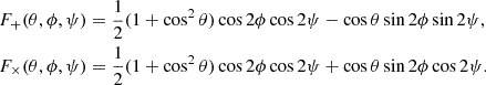
where F₊ and F_× are the ‘antenna pattern’ functions that define the dependence of the detector’s sensitivity on sky position and polarization angle, which can be expressed as (e.g. Dhurandhar & Tinto 1988)

$$\begin{array}{cc}& F_{+}(\theta ,\varphi ,\psi )=\frac{1}{2}(1+{cos}^2\theta )cos2\varphi cos2\psi -cos\theta sin2\varphi sin2\psi ,\hfill \\ \hfill & F_{\times }(\theta ,\varphi ,\psi )=\frac{1}{2}(1+{cos}^2\theta )cos2\varphi cos2\psi +cos\theta sin2\varphi cos2\psi .\hfill \end{array}$$(10)

The probability distribution of w for each detector is completely specified under the assumption of isotropic sky positions and binary orbital plane orientations. Since w ≤ 1, and given the dependencies in Eq. (8), for each detector there exists a ‘horizon’ distance, 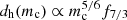$d_{\mathrm{h}}(m_{\mathrm{c}})\propto m_{\mathrm{c}}^{5/6}{f}_{7/3}$, such that ρ_opt(r = d_h) = ρ_lim, where ρ_lim is a minimum S/N required for a detection. This represents the distance beyond which a binary with a chirp mass, m_c, cannot be detected. Hence, for a given binary, one can write the S/N in the i-th detector of a network as

$$\begin{array}{c}\hfill {\rho }_i=w_i{\rho }_{\lim }\frac{d_{\mathrm{h},i}}{r},\end{array}$$(11)

and the squared ‘network S/N′ in an n-detector network as

$$\begin{array}{c}\hfill {\rho }_{\mathrm{net}}^2={\displaystyle \sum _{i=0}^{n-1}}{\rho }_i^2=w_0^2{\rho }_{\lim }^2\frac{d_{\mathrm{h},0}^2}{r^2}[1+{\displaystyle \sum _{i=1}^{n-1}}{\left(\frac{w_i}{w_0}\right)}^2{\left(\frac{d_{\mathrm{h},i}}{d_{\mathrm{h},0}}\right)}^2].\end{array}$$(12)

Let us now represent the detection as a threshold on the network S/N, ρ_net ≥ ρ_lim. In other words, let us define the detection probability of a binary merger as

$$\begin{array}{c}\hfill p_{\det }=\mathrm{\Theta }({\rho }_{\mathrm{net}}-{\rho }_{\lim }),\end{array}$$(13)

where Θ is the Heaviside step function. The effective sensitive volume of the network, neglecting cosmological effects, is then obtained by integrating the detection probability over volume and over the binary orientations,

$$\begin{array}{cc}\hfill V_{\mathrm{eff}}& =r^2{p}_{\det }\mathrm{d}rsin\theta \mathrm{d}\theta \mathrm{d}\varphi \frac{sin\iota \mathrm{d}\iota }{2}\frac{\mathrm{d}\psi }{2\pi }\hfill \\ \hfill & =4\pi d_{\mathrm{h},0}^3{x}^2\mathrm{\Theta }(\frac{{\rho }_{\mathrm{net}}}{{\rho }_{\lim }}-1)\mathrm{d}x\frac{sin\theta \mathrm{d}\theta }{2}\frac{\mathrm{d}\varphi }{2\pi }\frac{sin\iota \mathrm{d}\iota }{2}\frac{\mathrm{d}\psi }{2\pi }\hfill \\ \hfill & =\frac{4\pi }{3}{d}_{\mathrm{h},0}^3\langle x_{\lim }^3\rangle ,\hfill \end{array}$$(14)

where I defined the dimensionless distance x = r/d_h, 0 and its limiting value for detection at a fixed sky position and inclination (which follows from Eq. 12),

$$\begin{array}{c}\hfill x_{\lim }(\theta ,\varphi ,\iota ,\psi )=w_0(\theta ,\varphi ,\psi ){[1+{\displaystyle \sum _{i=1}^{n-1}}{\left(\frac{w_i({\stackrel{\sim }{\theta }}_i,{\stackrel{\sim }{\varphi }}_i,\iota ,{\stackrel{\sim }{\psi }}_i)}{w_0(\theta ,\varphi ,\iota ,\psi )}\right)}^2{\left(\frac{d_{\mathrm{h},i}}{d_{\mathrm{h},0}}\right)}^2]}^{1/2}.\end{array}$$(15)

In the above expression, $({\stackrel{\sim }{\theta }}_i,{\stackrel{\sim }{\varphi }}_i)$ and ${\stackrel{\sim }{\psi }}_i$ represent the sky position and the polarization angle as seen by detector i, as opposed to (θ, ϕ) and ψ, which pertain to the reference detector, 0. The average ⟨x_lim³⟩ is over isotropic sky positions and orientations. We call such an average the ‘geometrical factor’ of the network. This is related to the ‘peanut factor’, f_p, defined in Chen et al. (2021) through f_p = ⟨x_lim³⟩^−1/3. For n = 1, ⟨x_lim³⟩^−1/3 = f_p = 2.264 is the usual horizon-to-range ratio (Finn & Chernoff 1993; Chen et al. 2021).

For each detector, the BNS range, ℛ, can be defined as the radius of an Euclidean sphere whose volume is equal to the V_eff obtained considering only that single detector. Clearly, ℛ_i ∝ d_h, i (Chen et al. 2021). In particular, the relation between the horizon and the range can be expressed as d_h, 0 = 2.264ℛ₀(m_c/m_c, ref)^5/6, where m_c, ref = 1.22 M_⊙ (Chen et al. 2021) is the reference chirp mass for which the BNS range is conventionally defined (that corresponds to an equal-mass binary with m₁ = m₂ = 1.4 M_⊙).

For each pair of detectors, i and j, the probability distribution of the ratio

$$\begin{array}{c}\hfill \frac{w_i}{w_j}=\frac{F_{+,i}^2{(1+{cos}^2\iota )}^2+4F_{\times ,i}^2{cos}^2\iota }{F_{+,j}^2{(1+{cos}^2\iota )}^2+4F_{\times ,j}^2{cos}^2\iota }\end{array}$$(16)

depends only on the relative orientations of the two detectors. Samples of such a distribution can be obtained in a simple way by sampling isotropic sky positions and binary orientations, computing the antenna pattern functions of the two detectors for each sampled configuration, and constructing the ratio as expressed in the above equation. The resulting samples of the ratio can then be used to compute the geometrical factor ⟨x_lim³⟩ with a Monte-Carlo sum. These facts allow us to compute the effective sensitive volume of a network to a binary of chirp mass m_c by knowing only the detector orientations and their BNS ranges.

Since the duty cycle of the GW detectors is not 100%, at any time the GW detector network effectively acts as one of several possible sub-networks, depending on which combination of detectors is online. The formalism outlined above can be used to compute the effective sensitive volume of each of the sub-networks, and these can then be combined based on the fraction of time, in a given observing run, over which that particular sub-network was operating. From basic combinatorics, the number of sub-networks (i.e. possible combinations of online detectors) is

$$\begin{array}{c}\hfill N_{\mathrm{c}}(n)={\displaystyle \sum _{k=1}^n}\left(\begin{array}{c}n\\ k\end{array}\right),\end{array}$$(17)

where the sum is over n-choose-k Binomial coefficients. For a three-detector network, this is N_c(3) = 3 + 3 + 1 = 7. For the HLV network, these seven combinations are H, L, V, HL, LV, VH, and HLV. Let us number the observing runs of the GW detector network by an index, l, and denote by n_l the number of detectors that participated in each run. If f_l, j is the fraction of run l’s time during which only the combination j of detectors was online (the others being offline or presenting data quality issues), then the total effective sensitive volume of the run is

$$\begin{array}{c}\hfill V_l={\displaystyle \sum _{j=0}^{N_{\mathrm{c}}(n_l)-1}}{f}_{j,l}{V}_{\mathrm{eff},j,l}=\frac{4\pi }{3}{d}_{\mathrm{h},0,0,l}^3{\displaystyle \sum _{j=0}^{N_{\mathrm{c}}(n_l)-1}}{f}_{j,l}{\left(\frac{{\mathcal{R}}_{0,j,l}}{{\mathcal{R}}_{0,0,l}}\right)}^3{\langle x_{\lim }^3\rangle }_{j,l},\end{array}$$(18)

where ℛ_i, j, l is the BNS range of i-th detector of combination j during run l, and similarly d_{h, i, j, l} is the corresponding horizon distance. In order to obtain this expression, I made use of Eq. (14) and of the proportionality between horizon and range.

I note that the ratio of two effective sensitive volumes is independent of chirp mass, owing to the fact that the single-detector horizons (which are the only dimensional terms in Eq. (18)) all share the same dependency, $d_{\mathrm{h},0,0,l}\propto m_{\mathrm{c}}^{5/6}$. This shows that the detection rate estimate based on Eq. (6) is insensitive to the mass distribution of the binaries of interest, as long as their S/N is reasonably well approximated by that of an inspiral of two point masses.

3.2. Application to BNS and NSBH mergers in O4

Equation (18) allows us to write the ratio of expected numbers of BNS mergers, 𝒞 (Eq. 7), as a function of the BNS ranges of the detectors in each of the runs (which we assume to be constant across the runs for simplicity), the duration of the runs, and the sub-network time fractions, f_j, l. The duration of the runs and the representative BNS ranges of the detectors that I adopted for the calculations are reported in Table 1. These are based on the BNS range plots for each run and each detector reported in the observing run summary pages of the public Gravitational Wave Open Science (GWOSC) website³, and are representative values close to the peaks of the distributions of ranges reported there. Let me note here that LVK officially divides O4 into three parts; namely, O4a (May 24, 2023 to January 16, 2024), O4b (April 10, 2024 to January 28, 2025) and O4c (January 28, 2025 to November 18, 2025, according to the latest plan update). After the first nine weeks (63 d) of O4c, a long hiatus took place between April 1 and June 11: for that reason, I found it clearer to divide O4c into two parts, which I indicate with O4c1 (63 days from January 28 to April 1, 2025) and O4c2 (160 days from June 11 to November 18, 2025), removing the hiatus. In what follows, I present the results assuming this division.

For O4c, I assumed the same ranges as in O4b. In order to compute the sub-network time fractions for O1, O2, and O3, I retrieved the list of time segments that pass quality checks for the search of compact binary coalescences for each detector and each run from the GWOSC website⁴. This allowed me to extract the fraction of each run’s time over which each sub-network was available. For O4, these time segment lists are not yet available; therefore, I estimated the sub-network time fractions using the limited information available in the GWOSC, following the method described in Appendix A. The result is reported in Table 2, along with the geometrical factors computed using the ranges from Table 1.

Using the time volumes in Table 1, we can finally compute the 𝒞 ratio for some cases of interest. First of all, the ratio of the time volume expected to be span in O4c2 with respect to that surveyed up to O4c1 is

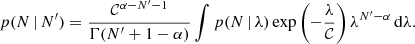
$$\begin{array}{c}\hfill \mathcal{C}=\frac{V{T}_{\mathrm{O}4\mathrm{c}2}}{V{T}_{\mathrm{O}1\to \mathrm{O}4\mathrm{c}1}}\approx 0.23.\end{array}$$(19)

Assuming the number of previous detection to be N′ = 2, and using Eq. (6), this leads to the O4c2 BNS detection probabilities shown with red squares in Figure 1, adopting the Jeffreys prior (i.e. setting α = 1/2). While the most likely outcome is, not surprisingly, the absence of new BNS detections, the computation shows that there is still a 40% probability of at least one BNS detection in O4c. For 0 ≤ α ≤ 1, this probability varies in the range of 34%−46%.

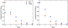Fig. 1. BNS and NSBH merger detection probability in O4c. The red squares in the left-hand panel show the probability that exactly NO4c2 BNS mergers are detected by the LVK network during O4c2, based on the number N′ = 2 detected in previous runs, according to Eq. (6) and adopting the Jeffreys prior (α = 1/2). The blue circles refer to NSBH instead, assuming N′ = 5. In the right-hand panel, the probability of a number of detections equal or greater than a given minimum, N ≥ NO4c2 in O4c2, is shown for the same two classes of sources.

The same approach can be applied to NSBH mergers, with the caveat that the inspiral-dominated signal approximation can introduce some (small) systematic bias, as can the fact that cosmological effects are neglected in the calculation. For these sources, I assumed N′ = 5, which corresponds to the two NSBH candidates with a false alarm rate (FAR)) lower than 1/4 yr in the GWTC-3 catalogue (Abbott et al. 2023a) plus the low-mass NSBH candidate GW230529_181500 (Abac et al. 2024) and the two candidates S250206dm and S241109bn released during O4 as ‘significant’ public alerts⁵ with an associated NSBH classification probability larger than 50%. Again adopting the Jeffreys prior, I obtained the results shown by blue circles in Figure 1, which show that the probability that O4c will yield at least one additional NSBH detection is around 68%, with N = 1 being the most likely outcome (only slightly more likely than N = 0). Adopting different priors affects the resulting probabilities by a few percent, spanning the range 64%−71% for 0 ≤ α ≤ 1.

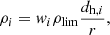
At any time, t, after the start of O4c2, we can also compute the probability of at least one detection in the remainder of the run (of duration T − t). This is obtained from

$$\begin{array}{cc}& p(N>0|N^{\prime },\alpha ,\mathcal{C}(t))\hfill \\ \hfill & =1-p(N=0|N^{\prime },\alpha ,\mathcal{C}=\left[\frac{1-\frac{t}{T}}{\mathcal{C}(0)\frac{t}{T}+1}\right]\mathcal{C}(0))\hfill \\ \hfill & =1-{\left(\frac{\mathcal{C}(0)+1}{\mathcal{C}(0)\frac{t}{T}+1}\right)}^{\alpha -1-N^{\prime }}.\hfill \end{array}$$(20)

Solid lines in Fig. 2 show the resulting probability for three different prior choices, α = 0, 1/2 and 1, keeping N′ = 2. The dashed grey line shows the result for α = 1/2 and N′ = 3, which represents the updated probability estimate of at least an additional fourth detection in the remainder of O4 after a hypothetical third detection has been made. The solid red line shows the result for NSBH mergers.

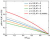Fig. 2. Probability of at least one detection in the remainder of O4, as a function of time, t, from the start of O4c2, for three different prior choices (different colours), keeping N′ = 2 fixed (i.e. assuming no detection, solid lines). The dashed line represents the probability of at least one hypothetical further detection after a third detection has been made during O4c2.

3.3. Updated local BNS merger rate density estimate

The time volumes calculated with the method described in this work can be used to provide an updated estimate of the local BNS merger rate density, R₀, based on GW observations. Using GW observational data up to the end of O3, based on the two BNS detections already discussed, and accounting for the uncertainty in the mass distribution of the merging component NSs, the LVK Collaboration estimated the true value of R₀ to lie in the range of 10 − 1700 Gpc⁻³ yr⁻¹, based on the union of the 90% credible ranges obtained from three different methods (Abbott et al. 2023b). Since the merger rate density estimate scales as R₀ = N′/VT, but N′ remained unchanged, this estimate can be updated simply by multiplying it by VT_new/VT_old. Using the time volumes in Table 1, I concluded that the absence of BNS merger detections in O4a and O4b reduces the estimate by a factor 3.55, leading to 2.8 Gpc⁻³ yr⁻¹ ≤ R₀ ≤ 480 Gpc⁻³ yr⁻¹. Due to the large uncertainty in models, this updated estimate remains in agreement with most predictions in the literature (Mandel & Broekgaarden 2022).

4. Predictions for O5

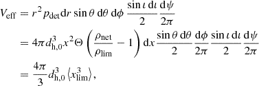
During the two years that will separate the end of O4c and the next observing run O5 of the LVK network, major upgrades are anticipated to lead to a greatly improved sensitivity, with a target LIGO BNS range of 330 Mpc, and a minimum target Virgo BNS range of 150 Mpc (Abbott et al. 2018b). The O5 run is anticipated to last for as long as three years. Adopting the same methodology as in the previous section (still neglecting the contribution of KAGRA), with these sensitivities and run duration, and assuming the same duty cycles as for O3b, the calculation gives a time volume to be surveyed for BNS mergers in O5 that is 12.6 times larger than the time volume at the end of O4 (see Table). Adopting 𝒞 = 12.6 and conservatively keeping N′ = 2 for BNS mergers and N′ = 5 for NSBH mergers, I obtained the O5 detection number probabilities shown in Figure 3. The greatly expanded range leads to much better detection prospects than O4. Using the median and the interval comprised between the 5^th and 95^th percentiles of the cumulative probability, we can predict the number of BNS detections in O5 to be $N_{\mathrm{BNS},\mathrm{O}5}={28}_{-21}^{+44}$, and the NSBH detections to be $N_{\mathrm{NSBH},\mathrm{O}5}={65}_{-38}^{+61}$. These estimates are lower by more than one order of magnitude with respect to those presented in Petrov et al. (2022), but they still demonstrate very promising prospects for multi-messenger astronomy in the next future. Clearly, they are based on a provisional estimate of the network sensitivity in O5, and hence will need to be updated once more accurate information will be available.

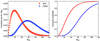Fig. 3. BNS merger detection probability in O5. The left-hand panel is the same as the corresponding panel in Fig. 1, but for O5. The right-hand panel shows the corresponding cumulative probability.

5. Discussion and conclusions

In this work I have presented a relatively simple method that aims to give reliable detection rate predictions to guide the astronomical community interested in the electromagnetic follow-up of BNS and NSBH mergers detected through their GWs, using publicly available information such as the BNS ranges of the detectors. The method clearly has some limitations. One of them stems from the fact that the sensitive volumes are estimated based on a simple representation of the GW detection condition as a threshold S/N. Actual search algorithms are more complex than this. In addition, the detector sensitivities typically vary during the runs. A much more accurate estimate of the surveyed time volume can only be obtained through the injection and recovery of simulated signals into the actual noise (e.g. Abbott et al. 2023a). The results of such injections in the future will allow the results presented here to be validated (or put into question).

The results presented here support the idea that GW170817 has been a particularly lucky statistical fluctuation. With more data, we see now that the average detection rate (and consequently the rate density) of BNS mergers is not as high as we could estimate eight years ago, but this is inherent to low-number statistics. Still, the probabilities derived in this work show that the next detection is just around the corner.

Acknowledgments

Some of the content of this work appeared earlier in an LVK technical note (https://dcc.ligo.org/P2400022/public) that was made public along with the April 18, 2024 update of the LVK Public Alerts User Guide website. I acknowledge the help I received at that time from colleagues in the LVK Collaboration who participated in the internal review of that document. I also thank Francesco Pannarale for pointing out some notation errors in that document, which I corrected in this work. I thank Andrew J. Levan for persuading me to seek publication of this work as a scientific article. I acknowledge funding by the Italian National Institute for Astrophysics (INAF) ‘Finanziamento per la Ricerca Fondamentale’ grant no. 1.05.23.04.04. This work has been funded by the European Union-Next Generation EU, PRIN 2022 RFF M4C21.1 (202298J7KT – PEACE).

References

Appendix A: Sub-network time fractions

From the summary pages⁶ of the O4a, O4b and O4c runs on the public GWOSC website we collected the following pieces of information: the fraction η_i, l of observing time of the i-th detector during the run, and the fraction of time ${\xi }_{k,l}^{\mathrm{GWOSC}}$ during which no interferometer (k = 0), only one interferometer (k = 1), two interferometers (k = 2) or three interferometers (k = 3) were observing (indicated as no-, single-, double- and triple-interferometer under the ‘network duty factor’ section of each summary page). This information is not sufficient to estimate the f_j, l fractions. To obviate to this, we assumed the following simple model of the network activity: for a fraction η_cd, l of the time, the network is in a coordinated downtime; for the remaining fraction (1 − η_cd, l) of the run, at any time each detector is independently active with a probability

$$\begin{array}{c}\hfill p_{\mathrm{act},i,l}=\frac{{\eta }_{i,l}}{1-{\eta }_{\mathrm{cd},l}},\end{array}$$(A.1)

where the constant at the denominator ensures that the detector’s total active time fraction is η_i, l as expected. Conversely, the probability of the detector being inactive is

$$\begin{array}{c}\hfill p_{\neg \mathrm{act},i,l}=1-p_{\mathrm{act},i,l}=1-\frac{{\eta }_{i,l}}{1-{\eta }_{\mathrm{cd},l}}=\frac{1-{\eta }_{i,l}-{\eta }_{\mathrm{cd},l}}{1-{\eta }_{\mathrm{cd}}}.\end{array}$$(A.2)

Let us now construct the n_l-uple (a_0, j, l, a_1, j, l, …, a_{nl − 1, j, l}) such that a_i, j, l = 1 if the i-th detector is active in configuration j during run l, and a_i, j, l = 0 otherwise. The sub-network time fraction predicted by the model is then

$$\begin{array}{cc}& f_{j,l}=(1-{\eta }_{\mathrm{cd},l}){\displaystyle \prod _{i=0}^{n_l-1}}{a}_{i,j,l}{p}_{\mathrm{act},i,l}+(1-a_{i,j,l})p_{\neg \mathrm{act},i,l}=\hfill \\ \hfill & ={(1-{\eta }_{\mathrm{cd},l})}^{1-n_l}{\displaystyle \prod _{i=0}^{n_l-1}}{a}_{i,j,l}{\eta }_{i,l}+(1-a_{i,j,l})(1-{\eta }_{i,l}-{\eta }_{\mathrm{cd},l})\hfill \end{array}$$(A.3)

For example, in O4a (which corresponds to l = 4) the configuration j = 0 corresponds to H being active while L is inactive, that is, (a_0, 0, 4, a_1, 0, 4) = (1, 0). Then we have f_0, 4 = η_0, 4(1 − η_1, 4 − η_cd, 4). Clearly, in each sub-network, the number of active detectors is

$$\begin{array}{c}\hfill n_{\mathrm{act},j,l}={\displaystyle \sum _{i=0}^{n_l-1}}{a}_{i,j,l}.\end{array}$$(A.4)

This implies that, for k ≥ 1, the model predicts

$$\begin{array}{c}\hfill {\xi }_{k,l}={\displaystyle \sum _{j=0}^{N_{\mathrm{c}}(n_l)-1}}{\delta }_{k,n_{\mathrm{act},j,l}}{f}_{j,l},\end{array}$$(A.5)

where δ_k, n is Kronecker’s delta. The remaining ξ_0, l can be obtained from the fact that ${\displaystyle \sum _{k=0}^{n_l}}{\xi }_{k,l}=1$. This shows that this simple model allows us to predict the fractions ξ_k, l by specifying the single parameter η_cd, l, once the individual detector duty cycles η_j, l are known. In order to choose the value of η_cd, l that provides the best match to the reported ${\xi }_{k,l}^{\mathrm{GWOSC}}$, we minimized the sum of the squared residuals between the actual and predicted fractions,

$$\begin{array}{c}\hfill \mathrm{\Psi }({\eta }_{\mathrm{cd},l})={\displaystyle \sum _{k=0}^{n_l}}{[{\xi }_{k,l}({\eta }_{\mathrm{cd},l})-{\xi }_{k,l}^{\mathrm{GWOSC}})]}^2.\end{array}$$(A.6)

This led to the values of the coordinated downtime fractions shown in Table A.1, which we used to compute the sub-network time fractions reported in Table 2 using Equation A.3.

All Tables

All Figures

Fig. 1. BNS and NSBH merger detection probability in O4c. The red squares in the left-hand panel show the probability that exactly NO4c2 BNS mergers are detected by the LVK network during O4c2, based on the number N′ = 2 detected in previous runs, according to Eq. (6) and adopting the Jeffreys prior (α = 1/2). The blue circles refer to NSBH instead, assuming N′ = 5. In the right-hand panel, the probability of a number of detections equal or greater than a given minimum, N ≥ NO4c2 in O4c2, is shown for the same two classes of sources.

In the text

	Fig. 2. Probability of at least one detection in the remainder of O4, as a function of time, t, from the start of O4c2, for three different prior choices (different colours), keeping N′ = 2 fixed (i.e. assuming no detection, solid lines). The dashed line represents the probability of at least one hypothetical further detection after a third detection has been made during O4c2.
In the text

	Fig. 3. BNS merger detection probability in O5. The left-hand panel is the same as the corresponding panel in Fig. 1, but for O5. The right-hand panel shows the corresponding cumulative probability.
In the text

References

- Abac, A. G., Abbott, R., Abouelfettouh, I., et al. 2024, ApJ, 970, L34 [CrossRef] [Google Scholar]
- Abbott, B. P., Abbott, R., Abbott, T. D., et al. 2017a, Phys. Rev. Lett., 119, 161101 [Google Scholar]
- Abbott, B. P., Abbott, R., Abbott, T. D., et al. 2017b, ApJ, 848, L12 [Google Scholar]
- Abbott, B. P., Abbott, R., Abbott, T. D., et al. 2017c, Nature, 551, 85 [Google Scholar]
- Abbott, B. P., Abbott, R., Abbott, T. D., et al. 2017d, ApJ, 848, L13 [CrossRef] [Google Scholar]
- Abbott, B. P., Abbott, R., Abbott, T. D., et al. 2018a, Phys. Rev. Lett., 121, 161101 [Google Scholar]
- Abbott, B. P., Abbott, R., Abbott, T. D., et al. 2018b, Living Rev. Rel., 21, 3 [NASA ADS] [CrossRef] [Google Scholar]
- Abbott, B. P., Abbott, R., Abbott, T. D., et al. 2019, Phys. Rev. Lett., 123, 011102 [Google Scholar]
- Abbott, R., Abbott, T. D., Acernese, F., et al. 2023a, Phys. Rev. X, 13, 041039 [Google Scholar]
- Abbott, R., Abbott, T. D., Acernese, F., et al. 2023b, Phys. Rev. X, 13, 011048 [NASA ADS] [Google Scholar]
- Acernese, F., Agathos, M., Agatsuma, K., et al. 2015, Class. Quant. Grav., 32, 024001 [Google Scholar]
- Baker, T., Bellini, E., Ferreira, P. G., et al. 2017, Phys. Rev. Lett., 119, 251301 [Google Scholar]
- Chen, H.-Y., Holz, D. E., Miller, J., et al. 2021, Class. Quant. Grav., 38, 055010 [NASA ADS] [CrossRef] [Google Scholar]
- Colombo, A., Salafia, O. S., Gabrielli, F., et al. 2022, ApJ, 937, 79 [NASA ADS] [CrossRef] [Google Scholar]
- Coulter, D. A., Foley, R. J., Kilpatrick, C. D., et al. 2017, Science, 358, 1556 [NASA ADS] [CrossRef] [Google Scholar]
- Creminelli, P., & Vernizzi, F. 2017, Phys. Rev. Lett., 119, 251302 [NASA ADS] [CrossRef] [Google Scholar]
- Dhurandhar, S. V., & Tinto, M. 1988, MNRAS, 234, 663 [Google Scholar]
- Dominik, M., Berti, E., O’Shaughnessy, R., et al. 2015, ApJ, 806, 263 [Google Scholar]
- Eichler, D., Livio, M., Piran, T., & Schramm, D. N. 1989, Nature, 340, 126 [NASA ADS] [CrossRef] [Google Scholar]
- Essick, R. 2023, Phys. Rev. D, 108, 043011 [Google Scholar]
- Finn, L. S., & Chernoff, D. F. 1993, Phys. Rev. D, 47, 2198 [NASA ADS] [CrossRef] [Google Scholar]
- Ghirlanda, G., Salafia, O. S., Paragi, Z., et al. 2019, Science, 363, 968 [NASA ADS] [CrossRef] [Google Scholar]
- Kajino, T., Aoki, W., Balantekin, A. B., et al. 2019, Progr. Part. Nucl. Phys., 107, 109 [NASA ADS] [CrossRef] [Google Scholar]
- Kasen, D., Metzger, B., Barnes, J., Quataert, E., & Ramirez-Ruiz, E. 2017, Nature, 551, 80 [Google Scholar]
- Kasliwal, M. M., Nakar, E., Singer, L. P., et al. 2017, Science, 358, 1559 [NASA ADS] [CrossRef] [Google Scholar]
- Kruckow, M. U., Tauris, T. M., Langer, N., Kramer, M., & Izzard, R. G. 2018, MNRAS, 481, 1908 [CrossRef] [Google Scholar]
- Lazzati, D., Deich, A., Morsony, B. J., & Workman, J. C. 2017, MNRAS, 471, 1652 [NASA ADS] [CrossRef] [Google Scholar]
- Li, L.-X., & Paczyński, B. 1998, ApJ, 507, L59 [NASA ADS] [CrossRef] [Google Scholar]
- LIGO Scientific Collaboration (Aasi, J., et al.) 2015, Class. Quant. Grav., 32, 074001 [Google Scholar]
- Mandel, I., & Broekgaarden, F. S. 2022, Liv. Rev. Relat., 25, 1 [Google Scholar]
- Mapelli, M., & Giacobbo, N. 2018, MNRAS, 479, 4391 [NASA ADS] [CrossRef] [Google Scholar]
- Margutti, R., & Chornock, R. 2021, ARA&A, 59, 155 [NASA ADS] [CrossRef] [Google Scholar]
- Metzger, B. D. 2020, Liv. Rev. Relat., 23, 1 [Google Scholar]
- Mooley, K. P., Deller, A. T., Gottlieb, O., et al. 2018, Nature, 561, 355 [Google Scholar]
- Nakar, E. 2020, Phys. Rep., 886, 1 [NASA ADS] [CrossRef] [Google Scholar]
- Nicholl, M., & Andreoni, I. 2025, Phil. Trans. Roy. Soc. London Ser. A, 383, 20240126 [Google Scholar]
- Petrov, P., Singer, L. P., Coughlin, M. W., et al. 2022, ApJ, 924, 54 [NASA ADS] [CrossRef] [Google Scholar]
- Pian, E., D’Avanzo, P., Benetti, S., et al. 2017, Nature, 551, 67 [Google Scholar]
- Ray, A., Camilo, M., Creighton, J., Ghosh, S., & Morisaki, S. 2023, Phys. Rev. D, 107, 043035 [Google Scholar]
- Savchenko, V., Ferrigno, C., Kuulkers, E., et al. 2017, ApJ, 848, L15 [NASA ADS] [CrossRef] [Google Scholar]
- Somiya, K. 2012, Class. Quant. Grav., 29, 124007 [NASA ADS] [CrossRef] [Google Scholar]