| Issue |
A&A
Volume 702, October 2025
|
|
|---|---|---|
| Article Number | A108 | |
| Number of page(s) | 8 | |
| Section | Extragalactic astronomy | |
| DOI | https://doi.org/10.1051/0004-6361/202556018 | |
| Published online | 10 October 2025 | |
Probing the farthest star clusters to the Small Magellanic Cloud
1
Instituto Interdisciplinario de Ciencias Básicas (ICB), CONICET-UNCuyo, Padre J. Contreras 1300, M5502JMA Mendoza, Argentina
2
Consejo Nacional de Investigaciones Científicas y Técnicas (CONICET), Godoy Cruz 2290, C1425FQB Buenos Aires, Argentina
⋆ Corresponding author: This email address is being protected from spambots. You need JavaScript enabled to view it.
Received:
18
June 2025
Accepted:
19
August 2025
Abstract
The Small Magellanic Cloud (SMC) has been tidally shaped by the interaction with the Large Magellanic Cloud (LMC). The scope of such an interaction was recently studied with regard to different astrophysical properties of its star cluster population, which point to star clusters placed, remarkably, outside the known extension of the galaxy. In this paper, we report results for three of the recently identified most external SMC star clusters, OGLE-CL-SMC0133, OGLE-CL-SMC0237, and Lindsay 116, using deep GEMINI GMOS imaging. Once we confidently cleaned their color-magnitude diagrams from field star contamination, we estimated their fundamental parameters by applying likelihood techniques. We also derived their structural parameters from normalized star-number-density radial profiles. Based on Gaia astrometric data, complemented by kinematics information available in the literature, we computed the 3D components of their space velocities. With similar ages (∼2.2 Gyr) and moderately metal-poor overall abundances ([Fe/H] = –1.0 to –0.7 dex), OGLE-CL-SMC0237 is placed 2.6 kpc from the SMC center and shares its disk rotation; OGLE-CL-SMC0133 is located 7.6 kpc from the galaxy center and exhibits a kinematics marginally similar to the SMC rotation disk, while Lindsay 116, placed 15.7 kpc from the center of the SMC, is facing strong perturbations of its orbital motion with respect to an ordered rotational trajectory. Furthermore, its internal dynamical evolution would seem to be accelerated – it seems kinematically older – in comparison with star clusters in the outskirts of relatively isolated galaxies. These outcomes lead to conclude that Lindsay 116 is subject to LMC tides.
Key words: techniques: photometric / Magellanic Clouds / galaxies: star clusters: general
© The Authors 2025
 Open Access article, published by EDP Sciences, under the terms of the Creative Commons Attribution License (https://creativecommons.org/licenses/by/4.0), which permits unrestricted use, distribution, and reproduction in any medium, provided the original work is properly cited.
This article is published in open access under the Subscribe to Open model. This email address is being protected from spambots. You need JavaScript enabled to view it. to support open access publication.
1. Introduction
Star clusters -groups of tens to thousand stars with a common origin in space and time- are important constituents of galaxies. Using their astrophysical properties (age, metallicity, heliocentric distance, etc.), it is possible to trace the formation and evolution of galaxies where their formed (see, e.g., Chilingarian & Asa’d 2018; Oliveira et al. 2023). The former is one of the most active fields of research in astrophysics, enriching our understanding how the Universe formed and evolved. Here, we paid attention to the Small Magellanic Cloud (SMC), which is, with the Large Magellanic Clouds, one of the closest galaxies to the Milky Way and deserves much of our attention concerning its population of star clusters.
The SMC is at a heliocentric distance of 62.50 kpc, and its depth is of ≈10 kpc (Ripepi et al. 2017; Muraveva et al. 2018; Graczyk et al. 2020). Illesca et al. (2025) analyzed the public 4m-class imaging SMASH survey database (Nidever et al. 2017) and found three SMC star clusters (OGLE-CL-SMC0133, OGLE-CL-SMC0237, and Lindsay 116) located along the galaxy line of sight with no previous distance estimates. Their resulting heliocentric distances place them remarkably outside the SMC at 21.8 kpc (OGLE-CL-SMC0133), 13.2 kpc (OGLE-CL-SMC0237), and 20.2 kpc (Lindsay 116) from the galaxy center, which enriches our understanding of the roles these star clusters have in the process of formation and evolution of the galaxy. As can be seen, they are between 2.7 up to 4.4 times farther from the SMC center than the outermost known SMC field stars.
Illesca et al. (2025) arrived to these results by fitting theoretical isochrones to the cluster color-magnitude diagrams (CMDs) – the deepest existing photometry at the time – once they had carefully removed the contamination of field stars by assigning cluster membership probability to each measured star by comparison with CMDs of their surrounding fields. However, the cluster CMDs show remarkably scattered and broad clusters’ features (S/N < 15) that led them to estimate heliocentric distances (d) with σ(d)/d ∼ 0.3. These uncertainties imply that the clusters could be part of the SMC main body within 1–2σ. In order to assess whether the clusters are in the SMC or outside it, σ(d)/d ∼ 0.05 is required, which in turn implies reaching S/N > 50 at the main-sequence turnoffs. Attempts to concretely reach S/N > 50 at the main-sequence turnoff of SMC star clusters similar to those analyzed by Illesca et al. (2025) have been achieved with 8m-class telescopes and high-spatial-resolution imaging instruments (see, e.g., Martínez-Vázquez et al. 2021).
The confirmation of the derived heliocentric distances of these three SMC star clusters, or a percentage of them, or even only one of them, opens the possibility to improve our understanding about the formation and evolution of the SMC and its dynamical interaction with other galaxies, among others. Star clusters with ages and metallicities compatible with being formed in the SMC and now located outside it, are witnesses of being stripped from galaxy interaction. Finding star clusters beyond the SMC body triggers the speculation that they could have been stripped from the interaction with the Large Magellanic Cloud (LMC). Indeed, Carpintero et al. (2013) performed simulations of the dynamical interaction between both Magellanic Clouds and their respective star cluster populations. Their models using a wide range of parameters for the orbits of both galaxies showed that approximately 15% of the SMC clusters were captured by the LMC. Furthermore, another 20–50% of its star clusters were ejected into the intergalactic medium. More recently, Piatti & Lucchini (2022) performed simulations of the orbit of the recently discovered stellar system YMCA-1 and found that it is a moderately old SMC star cluster that could be stolen by the LMC during any of the close interactions between both galaxies and now is seen to the east from the LMC center.
For the reasons mentioned above, we started an observational campaign with the aim of unveiling whether the three analyzed SMC star clusters are indeed far from the SMC. The new heliocentric distances derived in this work also contribute to building a statistically significant sample of SMC star clusters for a pending study of the structure of the cluster population in the SMC (Piatti 2023). Likewise, they give new insight into the large-scale structure of the area around the SMC. In Section 2, we describe the collected data and different procedures used to obtain the CMDs. Section 3 deals with the analysis of the star cluster CMDs from the employment of different cleaning tools, while in Section 4 we discuss the resulting clusters’ heliocentric distances. Section 5 summarizes the main conclusions of this work.
2. Observational data
We conducted imaging observations with the GEMINI South telescope and the GMOS-S instrument (3 × 1 mosaic of Hamamatsu CCDs; 5.5 × 5.5 square arcmin FOV; Allington-Smith et al. 2002; Hook et al. 2004; Gimeno et al. 2016) through g and i filters under program ID GS-2025A-FT-205 (PI: Piatti). We obtained eight images per filter and per star cluster in nights with excellent seeing (0.62″ to 0.97″ FWHM) and photometric conditions at a mean airmass of 1.9. We used individual exposure times of 155 s and 52 s for g and i filters, respectively, to prevent saturation. The SDSS standard fields E8_a F1, 140000-300000 F2 and PG1633+099 F2 were also observed alongside bias and sky-flat baseline observations. We reduced the data following the standard procedures (see documentation at the GEMINI Observatory web page)1 and employed the GMOS/GEMINI package in IRAF/GEMINI. We applied overscan, trimming, bias subtraction, flattening and mosaicing to all data images, with previously obtained nightly master calibration images (bias and flats). Then, we combined (added) all the program images for the same star cluster and filtered with the aim of gaining in reachable limiting magnitude. We found that the photometry depth increased more than one magnitude with respect to the photometry depth reached by single program images.
The photometry was obtained as outlined, for example, in Piatti (2022). We used routines in the DAOPHOT/ALLSTAR suite of programs (Stetson et al. 1990) to find stellar sources and to fit their brightness profiles with point-spread functions (PSFs) in order to obtain the stellar photometry of each summed image. For each of them, we obtained a preliminary PSF derived from the brightest, least contaminated ∼40 stars, which in turn was used to derive a quadratically varying PSF by fitting a larger sample of ∼100 stars. The two groups of PSF stars were selected looking at the image. Then, we used the ALLSTAR program to apply the resulting PSF to the identified stellar star clusters. ALLSTAR generates a subtracted image which we employed to find and measure magnitudes of additional fainter stars. We repeated this procedure three times for each summed image. Then, we combined all the independent g, i instrumental magnitudes using the stand-alone DAOMATCH and DAOMASTER programs2. As a result, we produced one data set per star cluster containing the x and y coordinates of each star, the instrumental g and i magnitudes with their respective errors, χ, and sharpness. With the aim of removing bad pixels, unresolved double stars, cosmic rays, and background galaxies from the photometric catalogs, we kept sources with |sharpness| < 0.5. The photometry of the surviving sources was put into the standard SDSS photometric system using the following transformation equations:
where g, i are the magnitudes in the standard SDSS photometric system, and  are the instrumental magnitudes measured by DAOPHOT/ALLSTAR (Stetson et al. 1990).
Figure 1 shows the final photometry for the entire GMOS FOV of the studied star clusters, which cover a relatively small central circular area with a radius of 0.80–1.60 arcmin (Bica et al. 2020). As can be seen, the CMDs resulted to be ∼2.5 up to 4.5 mag deeper than those retrieved by Illesca et al. (2025) from the SMASH database. They reveal the presence of a heavy field-star contamination composed of young-to-old stars.
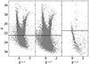 |
Fig. 1. CMDs of GMOS-S FOV centered on OGLE-CL-SMC0133 (left), OGLE-CL-SMC0237 (middle), and Lindsay 116 (right). The solid line represents the limiting magnitude reached by the SMASH database in those star cluster fields. |
3. CMD analysis
The presence of a star cluster in a star field implies the existence of a local stellar overdensity with distinctive magnitude and color distributions, whose stars delineate the cluster sequences in the CMD. Hence, the CMD observed along the cluster’s line of sight contains information concerning both cluster and field stars. This means that if the CMD features of the star field were subtracted, the intrinsic characteristics of the cluster CMD would be uncovered. One possibility of carrying out such a distinction consists of comparing a star field CMD with that observed along the cluster’s line of sight and then properly eliminating from the latter a number of stars equal to that found in the former. This scenario would also take into account that the magnitudes and colors of the eliminated stars in the cluster’s CMD must reproduce the respective magnitude and color distributions in the star-field CMD. The resulting decontaminated CMD should depict the intrinsic features of that cleaned particular field; such features, in the case of a star cluster, are the well-known star-cluster sequences.
We used a circular region around the centers of the studied star clusters with radii equal to 0.6′, 0.6′, and 1.0′ for OGLE-CL-SMC0133, OGLE-CL-SMC0237, and Lindsay 116, respectively, which were estimated from previously constructed stellar radial profiles based on star counts. Similarly, we devised 1000 star-field circles with the same radius of the star clusters’ circles and centered at four times the star clusters’ radii. They were randomly distributed around the star clusters’ circles. We then built the respective 1000 CMDs with the aim of considering the variation in the stellar density and in the magnitude and color distributions across the star clusters’ neighboring regions. The procedure to select stars to subtract from the star cluster CMD followed the precepts outlined by Piatti & Bica (2012). We applied it using one star field CMD at a time, comparing each one with the star cluster CMD. It consisted of defining boxes centered on the magnitude and color of each star of the star-field CMD; then, it superimposed the boxes on the star cluster CMD and finally chose one star per box to subtract. In order to guarantee that at least one star is found within the box boundary, we considered boxes of (Δg, Δ(g − i)) = (1.00 mag, 0.50 mag) in size. Whenever more than one star is found inside a box, the closest one to its center is removed. During the selection of the eliminated stars, we bore in mind their magnitude and color errors by allowing them to have 1000 different values of magnitude and color within an interval of ±1σ, where σ represents the errors in their magnitude and color, respectively. We also required that the spatial positions of the subtracted stars be chosen randomly. In practice, for each field star we randomly selected a position in the star cluster’s circle and searched for a star to subtract within a box of 0.1′ per side. We iterated this loop up to 1000 times if no star was found in the selected spatial box.
The outcome of the cleaning procedure is a CMD that likely only contains stars that represent the intrinsic features of that star cluster. From the 1000 different cleaned star cluster CMDs, we defined a probability, P (%), of there being star cluster magnitudes and colors as the ratio N/10, where N (between 0 and 1000) is the number of times a star was found among the 1000 different cleaned CMDs. Figure 2 shows the resulting cleaned CMDs for the three studied star clusters. They include all the stars measured within the star clusters’ radii, which are colored according to their respective P values. We note that the lack of field-star contamination reinforces the impression that the star cluster is actually far away from the SMC.
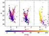 |
Fig. 2. CMDs of OGLE-CL-SMC0133 (left), OGLE-CL-SMC0237 (middle), and Lindsay 116 (right). The color bar represents (in %) how dissimilar the magnitude and color of a star are from the magnitude and color distributions of the projected surrounding SMC field-star population. |
We used the Automated Stellar Cluster Analysis code (ASteCA, Perren et al. 2015) to derive the star cluster’s fundamental parameters; namely age, heliocentric distance, and overall metallicity; we did so using stars with membership probabilities of P > 70%. In order to guide ASteCA, we adopted the mean and dispersion of E(V − B) values from the interpolation in the interstellar extinction map built by Schlafly & Finkbeiner (2011), provided by the NASA/IPAC Infrared Science Archive3, for the entire analyzed areas. ASteCA explores the parameter space of synthetic CMDs through the minimization of the likelihood function defined by Tremmel et al. (2013, the Poisson likelihood ratio (Eq. (10))) using a parallel tempering Bayesian MCMC algorithm, and the optimal-binning Knuth (2018) method. ASteCA relies on different compounds to generate the synthetic CMDs. Among them, it uses the theoretical isochrones computed by Bressan et al. (2012, PARSEC v1.2S4), the initial mass function of Kroupa (2002), as well as cluster masses in the 100–5000 M⊙ range, whereas binary fractions are allowed in the 0.0–0.5 range, with a minimum mass ratio of 0.5. Table 1 lists the resulting cluster astrophysical properties and the associated uncertainties, while Figure 3 shows the respective theoretical isochrones superimposed onto the star cluster CMDs constructed for stars with a membership probability of P > 70%.
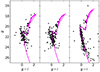 |
Fig. 3. CMDs of OGLE-CL-SMC0133 (left), OGLE-CL-SMC0237 (middle), and Lindsay 116 (right) for stars with P > 70%, with the isochrone of Bressan et al. (2012, PARSEC v1.2S) corresponding to the best-fit-parameter values superimposed (see text for details). |
Astrophysical and structural parameters of SMC star clusters.
4. Star cluster properties
We took advantage of our deeper GEMINI GMOS images to build star number-density radial profiles for the three studied star clusters. In order to do that, we counted the number of stars distributed inside boxes distributed across the entire observed star-cluster fields. We built several radial profiles, using, for each one, boxes of a fixed size (from 0.03′ up to 0.15′ per side) that increases in steps of 0.03′ per side. We then averaged all the constructed radial profiles and estimated their dispersion. As expected, the individual radial profiles built from star counts performed using smaller boxes resulted smoother toward the innermost clusters’ regions, while those obtained from larger boxes, traced the ample clusters’ surrounding fields better. Figure 4 depicts the resulting star cluster radial profiles. We fit a horizontal line to the background level using points located across the whole background region and adopted the intersection between the observed radial profile and the fitted background level as the clusters’ radii (rcls, see Table 1). Extensive artificial star tests were previously performed by Piatti et al. (2014) on similar GMOS/GEMINI data; the authors found that the 50% completeness level is reached in the innermost regions of massive LMC star clusters at g ∼ 23.5 mag and i ∼ 23.8 mag, respectively. Hence, we concluded that our radial profiles for the present less populated and less crowded star clusters do not suffer from incompleteness. To assist the reader, Figure A.1 shows the star counts in g and i for three different intervals, namely (1) r < rc; (2) rc < r < rcls; and (3) r > rcls, for OGLE-CL-SMC0133, OGLE-CL-SMC0237, and Lindsay 116, respectively.
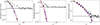 |
Fig. 4. Normalized observed and background-subtracted star number-density radial profiles of OGLE-CL-SMC0133 (left), OGLE-CL-SMC0237 (middle), and Lindsay 116 (right) drawn with open and black filled circles, respectively, with uncertainties represented by error bars. The horizontal line represents the adopted mean background level. Blue, orange, and magenta solid lines are the best-fit King (1962), Plummer (1911), and Elson et al. (1987) models, respectively. |
Finally, we fit three different models to the normalized background-subtracted radial profiles, namely the King (1962) profile model5, which was employed to derive core (rc) and tidal (rt) radii; the Plummer (1911) model, which helped to derive the half-light radius (rh) from the relation rh ∼ 1.3 × a6; and the Elson et al. (1987) model7, which gave rc ≈ b(22/γ − 1)1/2 and γ (γ is the power-law slope at large radii). Table 1 lists the resulting values of these structural parameters, while Figure 4 illustrates how they reproduce the star-cluster radial profiles.
We transformed the angular values of rc, rh, rt, and rcls to linear ones using the expression 2.9 10−4 × d × rc, h, t, where d is the star cluster’s heliocentric distance (see Table 1). We also derived the star cluster’s deprojected distance to the center of the SMC (in kpc) using the following relation:
 (1)
(1)
where dsmc is the heliocentric distance of the SMC center (62.5 ± 0.8 kpc, Graczyk et al. 2020).
We computed the star-cluster masses (log(M/M⊙)) using the relationships obtained by Maia et al. (2014, Equation (4)) as follows:
 (2)
(2)
where MI is the integrated absolute magnitude in the Johnson I filter (MI⊙ = 4.13 mag), and a and b are from Table 2 of Maia et al. (2014) for a representative SMC overall metallicity of Z = 0.004 (Piatti & Geisler 2013). The absolute integrated magnitudes were computed from the observed ones as follows:
 (3)
(3)
where I is the observed I integrated magnitude, and AI the mean interstellar absorption (AI = 1.85 E(B − V); see Table 1). The I values were obtained by transforming the measured SDSS g, i integrated magnitudes to the Johnson I photometric system using theoretical isochrones for the derived star clusters’ ages and metallicities (Bressan et al. 2012, PARSEC v1.2). The star-cluster integrated magnitudes were obtained by producing integrated SDSS g, i magnitude growth curves from our final photometry (see Section 2). Typical uncertainties were σ(log(M/M⊙)) ≈ 0.2.
We also calculated half-light relaxation times using the equation of Spitzer & Hart (1971):
 (4)
(4)
where  is the average mass of the cluster stars, and units are as follows: [tr] = Myr; [rh] = pc; [masses] = M⊙. For simplicity, we assumed a constant average stellar mass of 1.25 M⊙, which corresponds to the average between the smallest and the largest one in the theoretical isochrones of Bressan et al. (2012), which are representative of the studied SMC star clusters. The uncertainties of the computed quantities from Eqs. (1)–(4) were obtained by performing a thousand Monte Carlo experiments from which we calculated the standard deviation. Table 1 lists the resulting star-cluster masses and relaxation times.
We used the Gaia DR3 database (Gaia Collaboration 2016; Babusiaux et al. 2023) to collect astrometric information with the aim of deriving the mean star-cluster proper motions in right ascension (pmra) and in declination (pmdec). In this respect, we followed the recipes outlined by Piatti (2021a). Briefly, we devised 1000 different adjacent fields as described in Section 2 and used their vector point diagrams (VPDs) to decontaminate that of the respective star cluster. This is similar to what we did to clean the star clusters’ CMDs from field stars. From the 1000 different cleaned star clusters’ VPDs, we assigned cluster memberships and kept those with P > 70% as cluster stars. The mean cluster proper motions and dispersions were obtained from applying a likelihood approach (Pryor & Meylan 1993; Walker et al. 2006). The resulting values are listed in Table 1. Then, we searched the literature for mean star clusters’ radial velocities (Parisi et al. 2009, 2015, 2009), which, alongside mean proper motions and heliocentric distances, allowed us to compute the three components of the space velocity vector by employing the transformation Equations (9), (13), and (21) of van der Marel et al. (2002). We also computed the three space velocity components of a point placed at the star-cluster heliocentric distance that rotates according to the SMC rotation disk derived by Piatti (2021a). The difference between the 3D star-cluster velocity components and those of the corresponding position on the galaxy rotation disk, added in quadrature, was introduced by Piatti (2021b) and is called the “residual-velocity” index (ΔV). We found values of ΔV equal to 69.4 ± 22.0, 25.1 ± 20.0, and 224.0 ± 25 km/s, for OGLE-CL-SMC0133, 0237, and Lindsay 116, respectively.
5. Discussion
The three studied star clusters are projected onto different SMC composite star fields. As shown in the left panel of Figure 5, OGLE-CL-SMC0133 is located toward the northern edge of the SMC bar, such that a numerous population of young stars is expected to contaminate its CMD. OGLE-CL-SMC0237 is ∼2.5′ away from NGC 376’s center, a massive young SMC star cluster (Milone et al. 2023), while Lindsay 116 is located in the outermost halo of the SMC. Their CMDs witness the aforementioned star contamination (see Figure 2). Particularly, the brighter and low-membership-probability stars (P < 10%) in the CMDs of OGLE-CL-SMC0133 and OGLE-CL-SMC0237 likely come from the young SMC star-field population and from NGC 376, respectively. Indeed, some residuals from these stars remain in the cleaned star clusters’ CMDs (Figure 3). Nevertheless, the main star-cluster features are clearly distinguishable.
The derived ages and overall metallicities for the star-cluster sample are in very good agreement with the values available in the literature and with the recent estimates obtained by Illesca et al. (2025). Particularly, the difference between their ages and metal contents and the present ones resulted to be Δ(log(age/yr)) = –0.01 ± 0.05 and Δ[Fe/H] = –0.05 ± 0.12 dex, respectively. As for the heliocentric distances, Illesca et al. (2025) derived distances of 51.1, 75.2, and 42.3 kpc for OGLE-CL-SMC0133, 0237, and Linsday 116, respectively. Assuming that the SMC is at a mean distance of 62.5 kpc (Graczyk et al. 2020), our values (see Table 1) imply that the star clusters are closer to the center of theSMC. Because the SMC is more extended along the line of sight and that the line-of-sight depth is ∼10 kpc, with an average depth of 4.3 ± 1.0 kpc (Ripepi et al. 2017; Muraveva et al. 2018, and references therein), the new heliocentric distances put theclusters inside the SMC body. Because Illesca et al. (2025) derived heliocentric distances using ASteCA, we discard any difference originated from distinct methodological approaches. Instead, we think that they are the result of using shallower and deeper star clusters’ CMDs.
We analyzed the distribution of the heliocentric distances (d) of OGLE-CL-SMC0133, 0237, and Lindsay 116 using an updated sample of SMC star clusters with distance estimates put into an homogeneous scale as a reference. For that purpose, we employed, as a starting point, the compilation of star cluster distances of Piatti (2023), to which we added the results of a recent search through the literature carried out by Illesca et al. (2025, their Table A.1). We finally gathered distance information of 47 SMC star clusters. The right panel of Figure 5 depicts their distance distribution, where we indicate the position of the adopted distance of the SMC center with a vertical solid line. As can be seen, the star clusters expand along the line of sight at nearly 20 kpc (from ∼50 kpc up to 70 kpc), with a larger percentage of them distributed throughout the closer galaxy hemisphere. OGLE-CL-SMC0133 and OGLE-CL-SMC0237 resulted to be located in the main body of the SMC, while Lindsay 116 turned out to be one of the closest star clusters to the Sun.
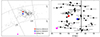 |
Fig. 5. Left: Equal-area Hammer projection of SMC in equatorial coordinates. Black dots represent the star clusters cataloged in Bica et al. (2020). Right: Distribution of heliocentric distances of SMC star clusters. The solid vertical line represents the SMC center derived by Graczyk et al. (2020). |
Figure 6 shows the spatial distribution of these star clusters as they appear projected in the sky, with their heliocentric distances distinguished by different colored symbols. They seem to occupy the SMC body, which makes them valuable in light of studies on the effects of the tidal interaction between both Magellanic Clouds. Indeed, Figure 6 suggests that star clusters spanning the whole range of line-of-sight depths are found throughout the entire SMC main body. However, there are seven star clusters with RA > 1.5 h – those closest in the sky to the LMC – that are among the nearest SMC star clusters to the Sun. In that region, there is no studied star cluster farther than ∼55 kpc from the Sun. This spatial closeness to the Sun of star clusters located on the easternmost side of the SMC is in very good agreement with the variation of distances of stars and gas in the region connecting the SMC and the LMC (Ripepi et al. 2017; Wagner-Kaiser & Sarajedini 2017; Omkumar et al. 2021). The LMC is at a mean heliocentric distance of 49.9 kpc (de Grijs et al. 2014), which implies that SMC star clusters affected by LMC tides could be found (in terms of heliocentric distances) closer to the Sun than the SMC.
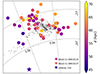 |
Fig. 6. Same as left panel of Figure 5, with colored symbols indicating star clusters with heliocentric distance estimates. Star symbols represent the star clusters studied. |
We probed to find whether the tidal interaction of the LMC with the SMC has left some imprints in the structures and kinematics of the studied SMC star clusters. At first glance, star clusters under the effects of stronger gravitational fields have differentially accelerated their internal dynamical evolution; i.e., they appear dynamically older. This behavior has been observed in Milky Way globular clusters (Piatti et al. 2019), LMC globular clusters (Piatti & Mackey 2018), and old SMC star clusters (Piatti 2025), which show their structural and dynamical parameters correlated with the distance to the galaxy center or with the tidal force strength. Star clusters toward the inner regions of these galaxies are in a more advanced stage of their internal dynamical evolution than those located in the outer galaxy regions. Particularly, the structural parameter c = log(rt/rc) and the ratio age/tr seem to decrease with increasing distances from the galaxy center. On the other hand, Piatti (2021b) proposed that the residual velocity of SMC star clusters is an index that can be used to disentangle whether they are affected by tidal effects caused by the LMC. He used the kinematics of 32 SMC star clusters projected toward known tidally perturbed SMC regions and found that their residual velocities are generally higher than those of SMC clusters projected toward the SMC main body (see his Figure 3). Indeed, residual velocities over ∼60 km/s suggest that star clusters are located in tidally perturbed regions or escaping the rotating disk kinematics. This residual velocity cut is in agreement with the SMC star cluster dispersion velocity ellipsoid, which has values of 50, 20, and 25 km/s along the right ascension, the declination, and the line-of-sight axes, respectively (Piatti 2021a).
As far as the residual velocity is considered, our resulting values strongly suggest that the larger the distance of a star cluster to the SMC center, the larger ΔV. OGLE-CL-SMC0237 is located at a deprojected distance of 2.6 kpc and rotates with the SMC disk. OGLE-CL-SMC0133, at 7.6 kpc from the SMC center, is marginally part of the rotating disk, while Lindsay 116 is largely confirmed as a star cluster escaping the SMC (rdeproj = 15.7 kpc). We note that these results come from a comparison of the 3D space velocities of the three clusters with the velocities they would have if they moved in the SMC rotational disk derived by Piatti (2021a) using star clusters, which, as far as we are aware, is a self-consistent comparison. Similar analyses could be attempted by using other derived SMC rotational disks (see, e.g., Zivick et al. 2018, 2019, 2021, and references therein); such analyses were not performed here because they are beyond the scope of this work. Because of the position in the sky of Lindsay 116, we speculate that it could be affected by LMC tides. Moreover, we examined the structural and dynamics parameter, c, and age/tr of the three studied star clusters and found that Lindsay 116 behaves as expected for a star cluster located in the inner region of the SMC; i.e., it would seem to be in a slightly more advanced dynamical evolutionary stage. Since Lindsay 116 is one of the outermost SMC star clusters, we think that the proximity to the LMC could be contributing to accelerating its internal dynamics. We note that the three studied star clusters have very similar ages that, in turn, agree very well with that of a star-cluster bursting formation event that took place ∼2.5 Gyr ag in both Magellanic Clouds, possibly as a result of a mutual close interaction (Piatti 2011a,b; Piatti & Geisler 2013). During such a bursting episode, the SMC (also the LMC) experienced an abrupt increase of its metal content, forming star clusters with [Fe/H] from ∼1.2 dex up to –0.6 dex. Nevertheless, according to different simulated orbits of the LMC/SMC, these galaxies could have experienced some other close encounter before the present time (Lucchini 2024, see Fig. 6 and references therein).
6. Conclusions
The SMC is known to have been interacting with the LMC since several gigayears ago (Rich et al. 2000; Bekki et al. 2004). Recently, Illesca et al. (2025) derived heliocentric distances of a sample of mostly unstudied SMC star clusters and found that some of them would be located notably outside the SMC main body. Because of the interacting nature of this pair of galaxies, the finding of star clusters orbiting their peripheries could witness the scope of such tidal interactions. The heliocentric distances estimated by Illesca et al. (2025) are based on SMASH DR2 data sets, which imply relatively shallow star-cluster CMDs. With the aim of confirming their estimated star-cluster heliocentric distances, we carried out GEMINI GMOS imaging observations, which, as far as we are aware, resulted in the deepest CMDs of OGLE-CL-SMC0133, 0237, and Lindsay 116 obtained so far. The analysis of these star clusters’ CMDs, in addition to structural parameters derived from stellar radial profiles also built from the acquired images and kinematics properties led us to conclude the following points.
-
We confirmed the recently estimated ages and overall metal content of the three studied star clusters OGLE-CL-SMC0133, 0237, and Lindsay 116. However, bearing in mind the 3D extension of the SMC, we found that they are located closer to the SMC center than previously thought. OGLE-CL-SMC0133 and 0237 are within the SMC main body, while Lindsay 116 is one of the farthest star cluster of the SMC.
-
When comparing their heliocentric distances with those of an up-to-date sample of star clusters with distance estimates put into a homogeneous scale, we found that the three studied star clusters mingle with the other star clusters; Lindsay 116 is highlighted as one of the most external star clusters of the galaxy. Hence, it could have been the subject of tidal stripping by the LMC.
-
The 3D spatial distribution of the 50 SMC star clusters with heliocentric distance estimates reveals that although star clusters are found spanning the whole line-of-sight depth in any direction toward the SMC, those located in the easternmost SMC regions (7 in total) are systematically closer to the Sun than the SMC center. Such a distance contrast is also seen in the spatial distribution of gas and stars connecting the SMC to the LMC.
-
Based on the behavior of the residual index (ΔV) as a function of the 3D positions of star clusters in the SMC found by Piatti (2021b), the presently derived ΔV values lead us to conclude that the kinematics of OGLE-CL-SMC0237 resembles that of the rotation of the SMC disk. Thus, OGLE-CL-SMC0133 would be marginally rotating with the SMC disk, while the kinematics of Lindsay 116 would seem to be largely perturbed compared to that of a rotational motion.
-
Some structural and dynamics properties of Lindsay 116 would also seem to be reached by tidal effects. Particularly, the concentration parameter c and the age/tr ratio obtained would point to a star cluster in an internal dynamical evolution stage compared to those located in the inner galactic regions. However, the loci of Lindsay 116 in the far SMC periphery would imply that an external gravitational potential has contributed to making the star cluster kinematically older.
Acknowledgments
We thank the referee for the thorough reading of the manuscript and timely suggestions to improve it. Based on observations obtained at the international GEMINI Observatory, a program of NSF NOIRLab, which is managed by the Association of Universities for Research in Astronomy (AURA) under a cooperative agreement with the U.S. National Science Foundation on behalf of the GEMINI Observatory partnership: the U.S. National Science Foundation (United States), National Research Council (Canada), Agencia Nacional de Investigación y Desarrollo (Chile), Ministerio de Ciencia, Tecnología e Innovación (Argentina), Ministério da Ciência, Tecnologia, Inovações e Comunicações (Brazil), and Korea Astronomy and Space Science Institute (Republic of Korea). Data for reproducing the figures and analysis in this work will be available upon request to the first author.
References
- Allington-Smith, J., Murray, G., Content, R., et al. 2002, PASP, 114, 892 [NASA ADS] [CrossRef] [Google Scholar]
- Babusiaux, C., Fabricius, C., Khanna, S., et al. 2023, A&A, 674, A32 [NASA ADS] [CrossRef] [EDP Sciences] [Google Scholar]
- Bekki, K., Couch, W. J., Beasley, M. A., et al. 2004, ApJ, 610, L93 [NASA ADS] [CrossRef] [Google Scholar]
- Bica, E., Westera, P., Kerber, L. d. O., et al. 2020, AJ, 159, 82 [Google Scholar]
- Bressan, A., Marigo, P., Girardi, L., et al. 2012, MNRAS, 427, 127 [NASA ADS] [CrossRef] [Google Scholar]
- Carpintero, D. D., Gómez, F. A., & Piatti, A. E. 2013, MNRAS, 435, L63 [Google Scholar]
- Chilingarian, I. V., & Asa’d, R. 2018, ApJ, 858, 63 [NASA ADS] [CrossRef] [Google Scholar]
- de Grijs, R., Wicker, J. E., & Bono, G. 2014, AJ, 147, 122 [Google Scholar]
- Elson, R. A. W., Fall, S. M., & Freeman, K. C. 1987, ApJ, 323, 54 [Google Scholar]
- Gaia Collaboration (Prusti, T., et al.) 2016, A&A, 595, A1 [NASA ADS] [CrossRef] [EDP Sciences] [Google Scholar]
- Gimeno, G., Roth, K., Chiboucas, K., et al. 2016, in Ground-based and Airborne Instrumentation for Astronomy VI, eds. C. J. Evans, L. Simard, & H. Takami, Society of Photo-Optical Instrumentation Engineers (SPIE) Conference Series, 9908, 99082S [NASA ADS] [Google Scholar]
- Graczyk, D., Pietrzyński, G., Thompson, I. B., et al. 2020, ApJ, 904, 13 [Google Scholar]
- Hook, I. M., Jørgensen, I., Allington-Smith, J. R., et al. 2004, PASP, 116, 425 [NASA ADS] [CrossRef] [Google Scholar]
- Illesca, D. M. F., Piatti, A. E., Chiarpotti, M., & Butrón, R. 2025, A&A, 696, A244 [NASA ADS] [CrossRef] [EDP Sciences] [Google Scholar]
- King, I. 1962, AJ, 67, 471 [Google Scholar]
- Knuth, K. H. 2018, Astrophysics Source Code Library [record ascl:1803.013] [Google Scholar]
- Kroupa, P. 2002, Science, 295, 82 [Google Scholar]
- Lucchini, S. 2024, Ap&SS, 369, 114 [Google Scholar]
- Maia, F. F. S., Piatti, A. E., & Santos, J. F. C. 2014, MNRAS, 437, 2005 [Google Scholar]
- Martínez-Vázquez, C. E., Salinas, R., & Vivas, A. K. 2021, AJ, 161, 120 [Google Scholar]
- Milone, A. P., Cordoni, G., Marino, A. F., et al. 2023, A&A, 672, A161 [NASA ADS] [CrossRef] [EDP Sciences] [Google Scholar]
- Muraveva, T., Subramanian, S., Clementini, G., et al. 2018, MNRAS, 473, 3131 [Google Scholar]
- Nidever, D. L., Olsen, K., Walker, A. R., et al. 2017, AJ, 154, 199 [Google Scholar]
- Oliveira, R. A. P., Maia, F. F. S., Barbuy, B., et al. 2023, MNRAS, 524, 2244 [NASA ADS] [CrossRef] [Google Scholar]
- Omkumar, A. O., Subramanian, S., Niederhofer, F., et al. 2021, MNRAS, 500, 2757 [Google Scholar]
- Parisi, M. C., Grocholski, A. J., Geisler, D., Sarajedini, A., & Clariá, J. J. 2009, AJ, 138, 517 [Google Scholar]
- Parisi, M. C., Geisler, D., Clariá, J. J., et al. 2015, AJ, 149, 154 [Google Scholar]
- Perren, G. I., Vázquez, R. A., & Piatti, A. E. 2015, A&A, 576, A6 [NASA ADS] [CrossRef] [EDP Sciences] [Google Scholar]
- Piatti, A. E. 2011a, MNRAS, 418, L40 [NASA ADS] [CrossRef] [Google Scholar]
- Piatti, A. E. 2011b, MNRAS, 418, L69 [NASA ADS] [Google Scholar]
- Piatti, A. E. 2021a, A&A, 650, A52 [NASA ADS] [CrossRef] [EDP Sciences] [Google Scholar]
- Piatti, A. E. 2021b, MNRAS, 508, 3748 [Google Scholar]
- Piatti, A. E. 2022, MNRAS, 511, L72 [NASA ADS] [CrossRef] [Google Scholar]
- Piatti, A. E. 2023, MNRAS, 526, 391 [Google Scholar]
- Piatti, A. E. 2025, MNRAS, 537, 1586 [Google Scholar]
- Piatti, A. E., & Bica, E. 2012, MNRAS, 425, 3085 [Google Scholar]
- Piatti, A. E., & Geisler, D. 2013, AJ, 145, 17 [Google Scholar]
- Piatti, A. E., & Lucchini, S. 2022, MNRAS, 515, 4005 [Google Scholar]
- Piatti, A. E., & Mackey, A. D. 2018, MNRAS, 478, 2164 [Google Scholar]
- Piatti, A. E., Keller, S. C., Mackey, A. D., & Da Costa, G. S. 2014, MNRAS, 444, 1425 [Google Scholar]
- Piatti, A. E., Webb, J. J., & Carlberg, R. G. 2019, MNRAS, 489, 4367 [Google Scholar]
- Plummer, H. C. 1911, MNRAS, 71, 460 [Google Scholar]
- Pryor, C., & Meylan, G. 1993, in Structure and Dynamics of Globular Clusters, eds. S. G. Djorgovski, & G. Meylan, Astronomical Society of the Pacific Conference Series, 50, 357 [Google Scholar]
- Rich, R. M., Shara, M., Fall, S. M., & Zurek, D. 2000, AJ, 119, 197 [Google Scholar]
- Ripepi, V., Cioni, M.-R. L., Moretti, M. I., et al. 2017, MNRAS, 472, 808 [Google Scholar]
- Schlafly, E. F., & Finkbeiner, D. P. 2011, ApJ, 737, 103 [Google Scholar]
- Spitzer, L., Jr., & Hart, M. H. 1971, ApJ, 164, 399 [NASA ADS] [CrossRef] [Google Scholar]
- Stetson, P. B., Davis, L. E., & Crabtree, D. R. 1990, in CCDs in Astronomy, ed. G. H. Jacoby, Astronomical Society of the Pacific Conference Series, 8, 289 [Google Scholar]
- Tremmel, M., Fragos, T., Lehmer, B. D., et al. 2013, ApJ, 766, 19 [Google Scholar]
- van der Marel, R. P., Alves, D. R., Hardy, E., & Suntzeff, N. B. 2002, AJ, 124, 2639 [NASA ADS] [CrossRef] [Google Scholar]
- Wagner-Kaiser, R., & Sarajedini, A. 2017, MNRAS, 466, 4138 [Google Scholar]
- Walker, M. G., Mateo, M., Olszewski, E. W., et al. 2006, AJ, 131, 2114 [Google Scholar]
- Zivick, P., Kallivayalil, N., van der Marel, R. P., et al. 2018, ApJ, 864, 55 [Google Scholar]
- Zivick, P., Kallivayalil, N., Besla, G., et al. 2019, ApJ, 874, 78 [Google Scholar]
- Zivick, P., Kallivayalil, N., & van der Marel, R. P. 2021, ApJ, 910, 36 [Google Scholar]
Appendix A: Photometric data properties
Figure A.1 shows the normalized star counts in g and i for different radial regimes.
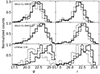 |
Fig. A.1. Normalized star counts for stars located at r < rc (dotted line), rc < r < rcls (dashed line), and r > rcls (solid line), respectively. |
Program kindly provided by P.B. Stetson.
 .
.
 .
.
 .
.
All Tables
All Figures
|
Fig. 1. CMDs of GMOS-S FOV centered on OGLE-CL-SMC0133 (left), OGLE-CL-SMC0237 (middle), and Lindsay 116 (right). The solid line represents the limiting magnitude reached by the SMASH database in those star cluster fields. |
| In the text | |
|
Fig. 2. CMDs of OGLE-CL-SMC0133 (left), OGLE-CL-SMC0237 (middle), and Lindsay 116 (right). The color bar represents (in %) how dissimilar the magnitude and color of a star are from the magnitude and color distributions of the projected surrounding SMC field-star population. |
| In the text | |
|
Fig. 3. CMDs of OGLE-CL-SMC0133 (left), OGLE-CL-SMC0237 (middle), and Lindsay 116 (right) for stars with P > 70%, with the isochrone of Bressan et al. (2012, PARSEC v1.2S) corresponding to the best-fit-parameter values superimposed (see text for details). |
| In the text | |
|
Fig. 4. Normalized observed and background-subtracted star number-density radial profiles of OGLE-CL-SMC0133 (left), OGLE-CL-SMC0237 (middle), and Lindsay 116 (right) drawn with open and black filled circles, respectively, with uncertainties represented by error bars. The horizontal line represents the adopted mean background level. Blue, orange, and magenta solid lines are the best-fit King (1962), Plummer (1911), and Elson et al. (1987) models, respectively. |
| In the text | |
|
Fig. 5. Left: Equal-area Hammer projection of SMC in equatorial coordinates. Black dots represent the star clusters cataloged in Bica et al. (2020). Right: Distribution of heliocentric distances of SMC star clusters. The solid vertical line represents the SMC center derived by Graczyk et al. (2020). |
| In the text | |
|
Fig. 6. Same as left panel of Figure 5, with colored symbols indicating star clusters with heliocentric distance estimates. Star symbols represent the star clusters studied. |
| In the text | |
|
Fig. A.1. Normalized star counts for stars located at r < rc (dotted line), rc < r < rcls (dashed line), and r > rcls (solid line), respectively. |
| In the text | |
Current usage metrics show cumulative count of Article Views (full-text article views including HTML views, PDF and ePub downloads, according to the available data) and Abstracts Views on Vision4Press platform.
Data correspond to usage on the plateform after 2015. The current usage metrics is available 48-96 hours after online publication and is updated daily on week days.
Initial download of the metrics may take a while.